2. Propulsion along the centreline

We first consider the case of an axisymmetric unbounded paraboloidal flow of strength $\tilde {U}_p$ whose stream function is given by $\tilde {\psi }_\infty = \tilde {U}_p r^4\sin ^4\theta /4$ (Jeong Reference Jeong2019) where the $(\;\tilde {}\;)$ denotes dimensional variables. The corresponding flow field becomes

(2.1)\begin{equation} \tilde{\boldsymbol{u}}_\infty = \left\langle \frac{1}{r^2\sin\theta}\frac{\partial\tilde{\psi}_\infty}{\partial\theta}, - \frac{1}{r\sin\theta}\frac{\partial\tilde{\psi}_\infty}{\partial r} \right\rangle = \tilde{U}_p\left\langle r^2\sin^2\cos\theta, -r^2\sin^3\theta \right\rangle. \end{equation}

The microswimmer is modelled as a squirmer with surface velocity (Lighthill Reference Lighthill1952; Blake Reference Blake1971; Pedley Reference Pedley2016)

(2.2)\begin{equation} \tilde{\boldsymbol{u}}_{sq} = \sum^\infty_{n=1}A_n P_n(\cos\theta)\boldsymbol{e}_r + \sum^\infty_{n=1}B_nV_n(\cos\theta)\boldsymbol{e}_\theta, \end{equation}

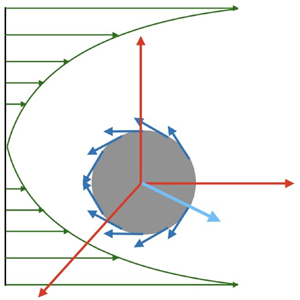
where $A_n$ and $B_n$ are the radial and tangential swimming modes, respectively, $P_n(\cos \theta )$ are the Legendre polynomials, $V_n(\cos \theta ) = -2/[n(n+1)] P^1_n(\cos \theta )$ and $P^1_n(\cos \theta )$ are the associated Legendre polynomials. The squirmer translates with velocity $\tilde {U}_s$ and is placed at the centreline of the paraboloidal flow (figure 1). Moreover, we consider the problem in the laboratory frame of reference where the origin of the coordinate system is taken to be at the centre of the squirmer with the parabolic flow evaluated at the origin. In this configuration, the squirmer is translating in a fluid that is quiescent in the far-field (Schonberg & Hinch Reference Schonberg and Hinch1989; Asmolov Reference Asmolov1999; Hood, Lee & Roper Reference Hood, Lee and Roper2015).

Figure 1. A squirmer with surface velocity $\boldsymbol {u}_{sq}$ propelling with velocity $U_s$ in an unbounded paraboloidal flow with velocity strength $U_p$. The squirmer is positioned at the centre of the background flow profile, translating along the $\boldsymbol {e}_z$ direction.

All equations governing the problem are scaled using the squirmer's radius $a$ for length, the first swimming mode $B_1$ for velocity, and the ratio $\mu B_1/a$ for pressure (where $\mu$ is the viscosity of the fluid). Note that in the case of a radial squirmer, $A_1$ is used in place of $B_1$. Given the size of the microswimmer, inertial effects can be omitted and the flow field is governed by the incompressible Stokes equation

(2.3a,b)\begin{equation} {-}\boldsymbol{\nabla} p + \nabla^2\boldsymbol{u} = \boldsymbol{0},\quad \boldsymbol{\nabla}\boldsymbol{\cdot}\boldsymbol{u} = 0, \end{equation}

where $p$ and $\boldsymbol {u}$ are the pressure and velocity fields of the fluid, respectively. The dimensionless squirmer's surface velocity

(2.4)\begin{equation} \boldsymbol{u}_{sq} = \sum^\infty_{n=1}\alpha_n P_n(\cos\theta)\boldsymbol{e}_r + \sum^\infty_{n=1}\beta_nV_n(\cos\theta)\boldsymbol{e}_\theta. \end{equation}

For a radial squirmer ($\beta _n=0$), $\alpha _n=A_n/A_1$ whereas $\beta _n=B_n/B_1$ for a tangential squirmer ($\alpha _n=0$). Note that the parameters $B_1$, $B_2$ and $B_3$ are associated with a Stokeslet, a stresslet and a Stokes quadrupole, respectively (Pak & Lauga Reference Pak and Lauga2014). Physically, the $B_1$ mode determines the propulsion speed while the $B_2$ mode dominates the far-field flow induced by the swimmer and, typically, captures the swimmer's typologies (neutral, pusher, puller). For this reason, many previous studies have neglected modes beyond $n=2$ (Zhu, Lauga & Brandt Reference Zhu, Lauga and Brandt2012; Chisholm et al. Reference Chisholm, Legendre, Lauga and Khair2016; Li, Lauga & Ardekani Reference Li, Lauga and Ardekani2021; Thery, Maab & Lauga Reference Thery, Maab and Lauga2023). The velocity field in the far-field is

(2.5)\begin{equation} \boldsymbol{u}(r\rightarrow\infty) = \boldsymbol{0}, \end{equation}

and

(2.6)\begin{equation} \boldsymbol{u}(r=1)=\boldsymbol{U}_s+\boldsymbol{u}_{sq} - \boldsymbol{u}_\infty, \end{equation}

on the surface of the squirmer where, after some algebraic manipulations, the dimensionless spatially varying paraboloidal flow can be expressed in the form

(2.7)\begin{equation} \boldsymbol{u}_\infty = U_p\left\langle r^2\left[ \tfrac{2}{5}\left(P_1(\cos\theta)-P_3(\cos\theta)\right)\right], - r^2\left[\tfrac{2}{15}\left(P^1_3(\cos\theta)-6P^1_1(\cos\theta)\right)\right] \right\rangle, \end{equation}

with $U_p = \tilde {U}_p/B_1$ (see Appendix A for details of the derivation). We deduce from (2.7) that the paraboloidal flow will affect the flow field up to order $n=3$. Thus, while previous studies in uniform flows have justifiably omitted swimming modes $B_{n\geq 3}$, here we consider a three-mode squirmer to fully characterise the effect of paraboloidal flows on swimming.

We use Lamb's general solution for the incompressible Stokes equation (Lamb Reference Lamb1945; Happel & Brenner Reference Happel and Brenner1973)

(2.8)$$\begin{gather} u_r = \sum^\infty_{n=0}\left(O_n r^{n+1} + Q_n r^{n-1} + \frac{R_n}{r^n} + \frac{S_n}{r^{n+2}}\right) P_n\left(\cos\theta\right), \end{gather}$$

(2.9)$$\begin{gather}u_\theta = \sum^\infty_{n=1}\left(-\frac{n+3}{2}O_n r^{n+1} - \frac{n+1}{2}Q_n r^{n-1} + \frac{n-2}{2}\frac{R_n}{r^n} + \frac{n}{2}\frac{S_n}{r^{n+2}}\right) V_n\left(\cos\theta\right) \end{gather}$$

and the boundary conditions to determine the exact flow and pressure fields. The coefficients $O_n, Q_n, R_n, S_n$ in the general solution are expressed in terms of the propulsion speed $U_s$ that, in turn, is obtained by applying the force-free condition on the surface of the squirmer $S$ $(r=1)$

(2.10)\begin{equation} \int_S \boldsymbol{\sigma}\boldsymbol{\cdot}\boldsymbol{n}\,{\rm d}S = \boldsymbol{0}, \end{equation}

where $\boldsymbol {\sigma }=-p\boldsymbol{\mathsf{I}} + \boldsymbol {\nabla }\boldsymbol {u}+(\boldsymbol {\nabla }\boldsymbol {u})^{\rm T}$, $\boldsymbol{\mathsf{I}}$ is the identity tensor and $\boldsymbol {n} = \boldsymbol {e}_r$ is the unit outward normal vector. In spherical coordinates the swimming direction $\boldsymbol {e}_z=\cos \theta \boldsymbol {e}_r-\sin \theta \boldsymbol {e}_\theta$, and (2.10) reduces to

(2.11)\begin{equation} \int^{2{\rm \pi}}_{0} \int^{\rm \pi}_{0} \left. \left( \sigma_{rr}\cos\theta - \sigma_{r\theta}\sin\theta \right) \right|_{r=1} \sin\theta\,{\rm d}\theta\,{\rm d}\phi = 0. \end{equation}

After lengthy calculations, (2.11) yields the propulsion speed

(2.12)\begin{equation} \tilde{U}_s = \tfrac{1}{3}\left[{-}A_1+2B_1 + 2U_p\left(A_1+B_1\right) \right]. \end{equation}

Equation (2.12) contrasts with the propulsion speed $\tilde {U}_{uniform}=(2B_1-A_1)/3$ of a spherical squirmer in a uniform flow (Lighthill Reference Lighthill1952; Blake Reference Blake1971). However, the speed remains independent of higher swimming modes $A_{n\geq 2}$ and $B_{n\geq 2}$. In keeping with previous studies, in the rest of our analysis we only consider the flow field generated by a squirmer with purely tangential surface velocity. The value $U_p=-1$ corresponds to the propulsion-free case, when the background flow is tuned to negate the first swimming mode $B_1$. This configuration is equivalent to the pumping problem (Pak & Lauga Reference Pak and Lauga2014), when the squirmer is held fixed and the flow field is generated solely as a result of interaction between the background flow and the surface velocity.

Substituting $U_s=2(1+U_p)/3$ and the coefficients $O_n, Q_n, R_n, S_n$ ($n\leq 3$) into the solutions, the flow field $\boldsymbol {u}=\langle u_r, u_\theta \rangle$ and pressure are obtained as

(2.13)\begin{align} u_r &= \frac{2 \cos\theta }{3 r^3}-\frac{\beta_2 \left(r^2-1\right) (3 \cos2 \theta+1)}{4 r^4}\nonumber\\ &\quad+\beta_3 \left[\frac{\cos \theta (5 \cos2 \theta -1)}{4 r^5}-\frac{\cos \theta (5 \cos2 \theta-1)}{4 r^3}\right] \nonumber\\ &\quad + U_p \frac{\left[3-r^2+3\left(7r^2-5\right)\cos2\theta\right]}{12r^5}\cos\theta, \end{align}

(2.14)\begin{align} u_\theta &= \frac{\sin \theta }{3 r^3} + \frac{\beta_2 \sin \theta \cos\theta }{r^4} -\frac{\beta_3 \left(r^2-3\right) \sin\theta (5 \cos2 \theta +3)}{16 r^5} \nonumber\\ &\quad + U_p \frac{\left[{-}27+19r^2+3\left(7r^2-15\right)\cos2\theta\right]}{48r^5}\sin\theta, \end{align}

(2.15)\begin{align} p & = \frac{\beta_2 ({-}24 r \cos 2 \theta -8 r)}{16 r^4}+\frac{\beta_3 ({-}15 \cos \theta-25 \cos3 \theta )}{16 r^4} + U_p \frac{7\left( 3\cos\theta+5\cos3\theta \right)}{16r^4}. \end{align}

Note that in the absence of a background flow ($U_p=0$), the velocity field reduces to that of a squirmer in a quiescent fluid (Lighthill Reference Lighthill1952; Blake Reference Blake1971). The velocity field can also be expressed in the form $\boldsymbol {u}=\langle \partial \psi /\partial \theta /(r^2\sin \theta ),-\partial \psi /\partial r/(r\sin \theta ) \rangle$ where the stream function

(2.16)\begin{align} \psi &= \frac{\sin ^2\theta}{3 r} -\frac{\beta_2 \left(r^2-1\right) \sin ^2\theta \cos \theta}{2 r^2}+\frac{\beta_3 \sin ^2\theta \left[{-}15 \left(r^2-1\right) \cos2 \theta -9 r^2+9\right]}{48 r^3} \nonumber\\ &\quad + U_p \frac{ \sin ^2\theta \left[3 \left(7 r^2-5\right) \cos 2 \theta +19 r^2-9\right]}{48 r^3}. \end{align}

To validate our results, we employed physics-informed neural networks (PINNs) to approximate the velocity field for $U_p=0$, and the propulsion speed $U_s$ for various values of the background flow's maximum velocity (see Appendix B for details). Recall again that paraboloidal flows only affect the first and third terms in Lamb's general solution. Therefore, for $n=2$ and $n\geq 4$, the velocity fields generated as a result of squirming in a paraboloidal flow and quiescent fluid are identical.

2.1. Flow field

The squirmer propels against the direction of the background flow. Thus, propulsion is along the positive (negative) $z$ direction when the background flow is directed towards the negative (positive) $z$ direction ($U_p<0$) [($U_p>0$)]. The flow field informs us on the types of hydrodynamic interactions between squirmers and other organisms/particles one can expect. We consider three cases to analyse the flow fields: $U_p=-2$, $U_p=-1$ (no propulsion) and $U_p=1$. Figure 2 shows the velocity magnitude and streamlines for a neutral squirmer (figure 2a–d) and a pusher with $\beta _2=-1$ (figure 2e–h). In a quiescent flow (figure 2a), neutral squirmers generate currents that advect particles in front of the swimmer away from the swimmer, whereas particles on the back of the swimmer are pulled towards the swimmer. This dynamics contrasts with that observed in a paraboloidal flow, as illustrated in figures 2(b)–2(d). In these cases, the situation is reversed: particles are drawn towards the swimmer at the front and driven away from its back. This behaviour is consistent across magnitudes of the background flow, including in the absence of propulsion when the flow cancels out the propulsion generated by the squirmer's surface velocity ($\hat {U}_p=B_1$). For pushers in a quiescent flow (figure 2e), particles are advected away from the swimmer both at the front and back, unless they are at the immediate vicinity of the swimmer's back, in which case the particles are pulled towards the swimmer. This overall dynamic is also observed in paraboloidal flows and across magnitudes of the background flow (figure 2f–h). The flow fields generated by three-mode squirmers show interesting and non-trivial variations that depend on the strength of the third mode $\beta _3$. This, in turn, has important implications on the hydrodynamic interactions experienced at the front and back of a three-mode squirmer. Figure 3 shows the velocity magnitude and streamlines for a three-mode squirmer with (figure 3a,b) $\beta _3=-1$ and (figure 3c–f) $\beta _3=-20$. At $\beta _3=-1$ in a uniform flow (figure 3a,c), the interaction dynamics is similar to that of a neutral squirmer: particles are repulsed at the front of the swimmer and attracted at the back. The dynamics is reversed in a paraboloidal flow (figure 3b,d), where this time particles move towards the swimmer's front whereas they are being advected away from its back. The flow field generated by the squirmer becomes nearly identical in uniform flows compared with paraboloidal flows when the magnitude of the swimming mode is increased. Figures 3(e) and 3(f) show the microvortices that are generated during the squirmer's motion. Although their features are similar, the velocity fields of the squirmers differ in their orientation. As a result, while the squirmer repels (draws in) particles at their front (back) in a quiescent fluid, it behaves in the opposite manner in a paraboloidal flow by pulling in (advecting away) particles at its front (back).

Figure 2. Velocity magnitude and streamlines for (a–d) a neutral squirmer ($\beta _2=0,\beta _3=0$) and (e–h) a pusher ($\beta _2=-1,\beta _3=0$) in a uniform flow (a,e) and in a paraboloidal flow with $U_p=-2$ (b,f), $U_p=-1$ (c,g) and $U_p=1$ (d,h). The streamlines extending through the axis of symmetry $x=0$ in (e,f,h) denote a separatrix: flow is directed towards the swimmer in the vicinity of the latter, and away from the swimmer in the far field. This is represented by the arrows. The colour bar represents the magnitude of the velocity field.

Figure 3. Velocity magnitude and streamlines for a three-mode squirmer with (a–d) $\beta _2=0,\beta _3=-1$ and (e,f) $\beta _2=0,\beta _3=-20$ in a uniform flow (a,c,e) and in a paraboloidal flow with $U_p=-2$ (b) and $U_p=1$ (d,f). The colour bar represents the magnitude of the velocity field. The ($\star$) symbols on either side of the squirmer in (b,f) denote the location of stagnation points, given by (2.17).

An interesting feature that also influences hydrodynamic interactions are vortices (or eddies). They have been reported for pushers and pullers with rotational velocities near a wall or flat plate (Drescher et al. Reference Drescher, Leptos, Tuval, Ishikawa, Pedley and Goldstein2009; Poddar, Bandopadhyay & Chakraborty Reference Poddar, Bandopadhyay and Chakraborty2020) and in the feeding patterns of starfish (Gilpin, Prakash & Prakash Reference Gilpin, Prakash and Prakash2017). In unbounded domains, these microvortices appear to be a signature of three-mode squirmers with large $\beta _3$ in both uniform flows (see Gilpin et al. (Reference Gilpin, Prakash and Prakash2017) and figure 3e) and paraboloidal flows (figure 3f).

Moreover, while microvortices are not present for three-mode squirmers in quiescent fluids with relatively small $\beta _3$, their presence in paraboloidal flows shows a dependence on the strength of the background flow. Specifically, microvortices are only observed for three-mode squirmers with small $\beta _3$ and $U_p<0$, as illustrated in figure 3(b). The existence of vortical regions in the flow field of neutral squirmers and pushers present yet another significant difference between propulsion in uniform flows vs paraboloidal flows. Indeed, the microvortices in figure 2(b,c) for neutral squirmers and figure 2(f) for pushers are a direct consequence of the paraboloidal flows. These flows introduce a Stokes quadrupole in the near-field, resulting in flow patterns similar to those generated by three-mode squirmers with small $\beta _3$ and $U_p<0$ (figure 3b) or more generally with large $\beta _3$ (figure 3f). Here we note that the flow field in a uniform flow has zero vorticity, whereas in a paraboloidal flow the vorticity $\boldsymbol {\nabla }\times \boldsymbol {u}\neq \boldsymbol {0}$. We further remark that vortices, like flow reversals, often point to stagnation points $(x^*, z^*) = (r_s\sin \theta,r_s\cos \theta )$ in the flow. For three-mode squirmers with $\beta _2=0$, figure 3(b,e,f) indicates that stagnation points exist along the $x$-axis ($\theta ={\rm \pi} /2$), where $u_r=0$. After setting $u_\theta =0$, the stagnation points are found to depend on the magnitude of the $\beta _3$ mode and on the strength of the background flow. The radius $r_s$ is given by

(2.17)\begin{equation} r_s ={\pm} 3\sqrt{\frac{\beta_3-U_p}{8+3\beta_3-U_p}}, \end{equation}

and the stagnation points are represented by the $\star$ symbols in figures 3(b) and 3(f).

2.2. Power dissipation and swimming efficiency

In this section, we discuss the work done by the squirmer and its efficiency. The power dissipation is given by $\mathcal {P}=-\int _S\boldsymbol {\sigma }\boldsymbol {\cdot }\boldsymbol {u}\boldsymbol {\cdot }\boldsymbol {n}\,{\rm d}S$. In spherical coordinates, $\mathcal {P}$ is expressed as

(2.18)\begin{equation} \mathcal{P} ={-}\int^{2{\rm \pi}}_{0} \int^{\rm \pi}_{0} \left. \left( \sigma_{rr}u_r + \sigma_{r\theta}u_\theta+\sigma_{r\phi}u_\phi \right) \right|_{r=1} \sin\theta\,{\rm d}\theta\,{\rm d}\phi. \end{equation}

Note that for the axisymmetric motion considered here, $\sigma _{r\phi }=0$, $u_\phi =0$. After some calculations, we obtain

(2.19)\begin{equation} \mathcal{P} = \frac{4{\rm \pi}}{105} \left\{70 \left(2+\beta_2 ^2\right)+35 \beta_3 ^2-U_p\left[ 38 \beta_3 -7 (16+7 U_p)\right]\right\}. \end{equation}

Equation (2.19) contrasts with the power dissipation $\mathcal {P}_{uniform} = 8{\rm \pi} (2+\beta _2^2+\beta _3^2/2)/3$ of a squirmer in a uniform flow (Lighthill Reference Lighthill1952; Blake Reference Blake1971). Moreover, we observe that the power dissipation varies not only as a function of the swimming modes, but also as a function of the background flow's strength. For a neutral squirmer ($\beta _2=\beta _3=0$) with $U_p=0$, we recover $\mathcal {P}_{uniform}=16{\rm \pi} /3$. When $U_p<-16/7$ or $U_p>0$, a neutral squirmer in a paraboloidal flow expends more energy compared with its counterpart in a uniform flow. However, swimming in a paraboloidal flow becomes more beneficial for the squirmer provided $U_p\in (-16/7,0)$. We can similarly compare the power dissipation for pushers/pullers ($\beta _3=0$) in paraboloidal flows relative to their work in uniform flows. Figure 4(a) shows the paraboloidal-to-uniform ratio $\varepsilon =\mathcal {P}/\mathcal {P}_{uniform}$ for a range of $\beta _2$ values with flow strength $U_p=-3$ (solid), $U_p=-2$ (dashed) and $U_p=1$ (dash-dotted). As expected from the analysis of the neutral squirmer, pushers/pullers always expend less energy compared with their counterparts in uniform flows for $U_p=-2$.

Figure 4. Paraboloidal-to-uniform ratios of (a) power dissipation and (b) swimming efficiency as a function of the $\beta _2$ swimming mode for various strengths of the paraboloidal background flow $U_p$.

Before discussing three-mode squirmers, we analyse the efficiency for two-mode squirmers. The swimming efficiency $\eta = F_DU_s/\mathcal {P}$ (Lighthill Reference Lighthill1952), where $F_D=F_D^p+F_D^s = 4{\rm \pi} U_p+6{\rm \pi} U_s$ is the force required to drag a rigid sphere at the swimming speed in the same fluid medium. Here, $F_D^p$ alone is the drag force experienced by a rigid sphere in a paraboloidal flow (Chwang & Wu Reference Chwang and Wu1975) while $F_D^s$ is the Stokes drag in the absence of a paraboloidal background flow. After some simplification, the efficiency is given by

(2.20)\begin{equation} \eta = \frac{70 (1+U_p) (1+2U_p)}{70 \left(2+\beta_2 ^2\right)+35 \beta_3 ^2-U_p\left[ 38 \beta_3 -7 (16+7 U_p)\right]}. \end{equation}

Figure 4(b) shows the ratio $\nu =\eta /\eta _{uniform}$ for the flow strengths in figure 4(a). In this case, the efficiency of a swimmer in a uniform flow is given by $\eta _{uniform} = 1/(2+\beta _2^2+\beta _3^2/2)$ (Lighthill Reference Lighthill1952; Blake Reference Blake1971). We conclude from the results that all two-mode squirmers in paraboloidal flows experience a gain in swimming efficiency ($\nu >1$), except for $U_p=-1/2,-1$. For $U_p=-1$ the efficiency is zero since the squirmer does not propel ($U_s=0$). On the other hand, efficiency is also zero when $U_p=-1/2$ (the drag forces $F_D^p$ and $F_D^s$ cancel each other out).

In the case of a three-mode squirmer, we produce the $\beta _2-\beta _3$ parameter space (figure 5) to determine the conditions under which the addition of the third swimming mode may yield behaviour distinct from that of a two-mode squirmer. In this analysis, we consider $U_p=-2$. On one hand, figure 5(a) shows that squirmers in a paraboloidal flow expend more energy when $\beta _3\gtrapprox 0.5$. On the other hand, while the ratio $\varepsilon$ may vary depending on $\beta _3$, figure 5(b) shows that $\nu >1$ for a three-mode squirmer. Thus, despite $\varepsilon$ being greater than unity, the three-mode squirmer is always a more efficient swimmer in paraboloidal flows compared with uniform flows.

Figure 5. Parameter space of $(\beta _2,\beta _3)$ for the paraboloidal-to-uniform ratios of power dissipation (a) and efficiency (b) for a three-mode squirmer with $U_p=-2$. The intersection of the vertical lines correspond to the combination $(\beta _2,\beta _3)$ at which a two-mode squirmer in a paraboloidal is a more ideal swimmer than a three-mode squirmer in a uniform flow.

The parameter spaces in figure 5 are subdivided into distinct spheroidal-shaped ‘holes’ or ‘sinks’, especially in the regions $\beta _3<0.5$ for the swimming efficiency (figure 5b). The smallest of these sinks $\mathcal {S}$ contains the combinations $(\beta _2,\beta _3)$ that minimise power dissipation and maximise swimming efficiency. The location of the epicentre of $\mathcal {S}$ is $(0,38U_p/35)$, as illustrated by the intersection of the dashed lines in figure 5. The case $\beta _3=38U_p/35$ corresponds to the non-zero value that eliminates the expression $35\beta _3^2-38U_p\beta _3$ in (2.19) and (2.20). In other words, at this value a three-mode squirmer in a paraboloidal flow expends the same energy and swims as efficiently as a two-mode squirmer subject to the same background flow. This suggests that squirmers in paraboloidal flows may be able to take advantage of the background flow to lower their rate of work and become more efficient swimmers. In terms of artificial microswimmers, our findings raise the possibility of novel design principles for microrobots that take advantage of specific properties of the background flow to reduce their work.

To conclude this section, we discuss the potential biological relevance of these results. The first swimming mode $B_1$ can be approximated using $B_1=3\tilde {U}_s/2$ where $\tilde {U}_s$ is obtained from experimental measurements of the velocity of various microorganisms including ciliates (Rodrigues, Lisicki & Lauga Reference Rodrigues, Lisicki and Lauga2021). Values of the $\beta _2=B_2/B_1$ swimming modes have been estimated previously for artificial and biological swimmers (Evans et al. Reference Evans, Ishikawa, Yamaguchi and Lauga2011). In general, they range from $-1$ ( Escherichia coli Drescher et al. Reference Drescher, Dunkel, Cisneros, Ganguly and Goldstein2011), to $\approx$0 (Volvox Short et al. (Reference Short, Solari, Ganguly, Powers, Kessler and Goldstein2006) and artificially created squirmers such as autonomous vesicles Miura et al. (Reference Miura, Oosawa, Sakai, Syundou, Ban and Shioi2010) or squirming droplets Thutupalli, Seemann & Herminghaus Reference Thutupalli, Seemann and Herminghaus2011), to 1 (Chlamydomonas Pedley & Kessler Reference Pedley and Kessler1990). This range of $\beta _2$ values lies squarely in the region of least power expenditure and greatest efficiency found in figure 5. Biological microorganisms naturally strive to optimise their motion, and our results capture this behaviour. To the best of the authors’ knowledge, measurements of higher swimming modes have not been performed on biological microorganisms. Moreover, higher modes lead to greater energy expenditure and less efficient swimming. Our results, however, raise the possibility of designing still-efficient artificial microswimmers. Specifically, the later can be built by accounting for the properties of the background flow such that adding a third swimming mode with $B_3\approx \tilde {U}_p$ does not increase (decrease) the power dissipation (swimming efficiency) of the microswimmer compared with a swimmer with only the first two modes. In addition to minimising work, the carefully added swimming gait could serve other purposes such as aiding in the transport of cargo (Ouyang et al. Reference Ouyang, Lin, Lin, Yu and Phan-Thien2023).

3. A note on the propulsion of an off-centred squirmer

Results presented in § 2 apply to the propulsion of a squirmer located on the centreline of the paraboloidal flow, in which case the swimmer can only propel along the background flow direction $\boldsymbol {e}_z$. For completeness, we now consider the case of a squirmer that is positioned off the centreline of the background flow. The latter is located at a distance $(x_0,y_0)$ from the origin (figure 6). We specifically focus on determining the translational and rotational velocities of the squirmer in this general case.

Figure 6. A squirmer with radius $a$ and surface velocity $\boldsymbol {u}_{sq}$ off the centreline of a paraboloidal flow located a distance $(x_0,y_0)$ from the origin.

The paraboloidal flow in Cartesian coordinates is given by (Chwang & Wu Reference Chwang and Wu1975)

(3.1)\begin{equation} \tilde{\boldsymbol{u}}_\infty = \bar{U}_{p}\left[\left(x-x_0\right)^2+\left(y-y_0\right)^2\right]\boldsymbol{e}_z. \end{equation}

Expanding the quadrating terms and simplifying yields the paraboloidal flow in spherical coordinates

(3.2)\begin{equation} \tilde{\boldsymbol{u}}_\infty = \bar{U}_{p}\left[r^2\sin^2\theta - r\sin\theta\left(\dot{\gamma}_1\cos\phi + \dot{\gamma}_2\sin\phi\right) + \varGamma \right]\boldsymbol{e}_z, \end{equation}

where $\dot {\gamma }_1=2x_0$ and $\dot {\gamma }_2=2y_0$ are local shear rates and $\varGamma =x_0^2+y_0^2$. Equation (3.2) reveals that in addition to the paraboloidal flow $\bar {U}_{p}r^2\sin ^2\theta \boldsymbol {e}_z$, the off-centred squirmer experiences a linear shear flow $-\bar {U}_{p}r\sin \theta (\dot {\gamma }_1\cos \phi + \dot {\gamma }_1\sin \phi ) \boldsymbol {e}_z$ and a uniform flow $\bar {U}_{p}\varGamma \boldsymbol {e}_z$ (Chwang & Wu Reference Chwang and Wu1975; Hanna & Vlahovska Reference Hanna and Vlahovska2010). We observe immediately that positioning the squirmer off the centreline of the background flow introduces a rotational motion in the azimuthal direction $\boldsymbol {e}_\phi$ that results from the linear shear flow. The boundary conditions in the laboratory frame become

(3.3)$$\begin{gather} \hat{\boldsymbol{u}}(r=a) = \hat{\boldsymbol{u}}_{sq} + \hat{\boldsymbol{U}}_s+\hat{\boldsymbol{\varOmega}}_s \times\boldsymbol{x}_s - \tilde{\boldsymbol{u}}_\infty, \end{gather}$$

(3.4)$$\begin{gather}\hat{\boldsymbol{u}}(r\rightarrow\infty) = \boldsymbol{0}, \end{gather}$$

where $\boldsymbol {x}_s = a\boldsymbol {e}_r$ and $\hat {\boldsymbol {\varOmega }}_s = \hat {\varOmega }_s\boldsymbol {e}_k$ is the rotational velocity of the squirmer obtained by imposing the torque-free condition

(3.5)\begin{equation} \int_S \boldsymbol{x}_s\times\left(\boldsymbol{\sigma}\boldsymbol{\cdot}\boldsymbol{n}\right){\rm d}S = \boldsymbol{0}. \end{equation}

As in § 2, the translational velocity $\hat {\boldsymbol {U}}_s = \hat {U}_s\boldsymbol {e}_k$ is obtained using the force-free condition (2.10). The index $k$ denotes the coordinates $x,y,z$, so the translational and rotational velocities can occur in any direction. The generalised surface velocity $\hat {\boldsymbol {u}}_{sq}$ for the purely tangential squirming motion is given by (Pak & Lauga Reference Pak and Lauga2014)

(3.6)\begin{align} u_{sq,r} & = 0 \end{align}

(3.7)\begin{align} u_{sq,\theta} &= \sum^\infty_{n=1} \sum^n_{m=0} \left[ -\frac{2\sin\theta P^{m'}_n}{na^{n+2}}\left( B_{mn}\cos m\phi + \hat{B}_{mn} \sin m\phi \right) \right. \nonumber\\ &\quad +\left. \frac{m P^m_n}{a^{n+1}\sin\theta} \left( \hat{C}_{mn}\cos m\phi - C_{mn} \sin m\phi \right) \right] \end{align}

(3.8)\begin{align} u_{sq,\phi} &= \sum^\infty_{n=1} \sum^n_{m=0} \left[ \frac{2m P^{m}_n}{na^{n+2}\sin\theta}\left( \hat{B}_{mn}\cos m\phi - B_{mn} \sin m\phi \right) \right. \nonumber\\ &\quad +\left. \frac{\sin\theta P^{m'}_n}{a^{n+1}} \left( C_{mn}\cos m\phi + \hat{C}_{mn} \sin m\phi \right) \right], \end{align}

where $P^m_n = P^m_n(\cos \theta )$ are the associated Legendre polynomials and $B_{mn}$, $\hat {B}_{mn}$, $C_{mn}$ and $\hat {C}_{mn}$ are the squirming modes.

We use Lamb's general solution for exterior problems (Pak & Lauga Reference Pak and Lauga2014) and apply the boundary conditions to obtain the velocity field $\boldsymbol {u}=\langle u_r,u_\theta,u_\phi \rangle$ for the general squirming motion of a three-mode squirmer (up to squirming modes $B_{03}$ and $C_{03}$) in paraboloidal flows. The components of the velocity field are given by (C5)–(C7) in Appendix C. After applying the force- and torque-free conditions ((2.10) and (3.5)), lengthy calculations yield the translational and rotational velocities

(3.9)$$\begin{gather} U_s = \frac{4}{3a^3}\left( B_{11}\boldsymbol{e}_x + \hat{B}_{11}\boldsymbol{e}_y - B_{01}\boldsymbol{e}_z \right) + \bar{U}_{p} \left( \frac{2}{3}a^2+\varGamma \right) \boldsymbol{e}_z, \end{gather}$$

(3.10)$$\begin{gather}\varOmega_s = \frac{1}{a^3}\left( C_{11}\boldsymbol{e}_x + \hat{C}_{11}\boldsymbol{e}_y - C_{01} \boldsymbol{e}_z \right). \end{gather}$$

The translational velocity due to purely tangential surface velocity in (2.12) is recovered by using a simple rescaling $B_{01}=-a^3B_1/2$, $\bar {U}_p = U_p/a^2$ and setting $\varGamma =0$, $B_{11}=\hat {B}_{11}=0$. Moreover, in the absence of a paraboloidal flow ($\bar {U}_p=0$) the translational and rotational velocities agree with the results obtained using the reciprocal theorem (Pak & Lauga Reference Pak and Lauga2014). Note that the propulsion of the off-centred squirmer becomes restricted to the $x-y$ plane when the strength of the paraboloidal flow $\bar {U}_p = 4 B_{01}/a^3(2a^2+3\varGamma )$.

The power dissipation is calculated using (2.18), and can be expressed in terms of contributions from the quiescent and background flows: $\mathcal {P} = \mathcal {P}_{uniform} + \mathcal {P}_{\bar {U}_p}$. In this case, $\mathcal {P}_{uniform}$ is the expression obtained by Pak & Lauga (Reference Pak and Lauga2014) for a non-axisymmetric squirmer (equation (77) in their paper) whereas $\mathcal {P}_{\bar {U}_p}$ is given by

(3.11)\begin{align} \mathcal{P}_{\bar{U}_p} &= {\rm \pi}\mu \left\{ -\frac{4}{105} \left[ 224B_{01} + \frac{72}{a^2}B_{03} - \frac{252}{a^2}\left( \dot{\gamma}_1 B_{12}+\dot{\gamma}_2\hat{B}_{12} \right) \right] \bar{U}_p\right. \nonumber\\ &\quad +\left. \frac{4 a^3}{105}\left[41a^2 + 42\left(\dot{\gamma}_1^2+\dot{\gamma}_2^2\right) \right] \bar{U}_p^2 \right\}. \end{align}

Equation (3.11) shows that the power dissipation depends explicitly on the linear shear flow, generated as a result of the position of the squirmer relative to the paraboloidal flow's centreline. This result contrasts with (3.9) and (3.10) that do not depend on the local shear rates $\dot {\gamma }_1$ or $\dot {\gamma }_2$, and suggest that the linear shear flow does not influence the translational and rotational velocities of the squirmer. In terms of the dependence on shear flow, our conclusion about the translational velocity is akin to the result obtained by Pak, Feng & Stone (Reference Pak, Feng and Stone2014) in the case of a surfactant-covered drop in a Poiseuille flow.

4. Concluding remarks

In this paper, we have investigated the propulsion of a spherical ciliated microorganism, represented by a squirmer, in a paraboloidal flow. First, we considered the axisymmetric problem. We have obtained exact analytical solutions of the propulsion speed, power dissipation, swimming efficiency, flow and pressure fields, and contrasted our results with those of Lighthill, the long-standing benchmark for microswimming studies in uniform flows. We have found that while the propulsion speed $U_s=2(1+U_p)/3$ only depends on the first swimming mode (as it does for propulsion in uniform flows first reported by Lighthill Reference Lighthill1952; Blake Reference Blake1971), it is now influenced by the strength of the background flow. The dependence on the maximum velocity of the paraboloidal flow played a significant role in the amount of work being experienced by the squirmer. However, although we have determined the range of flow strength that minimises work, we have shown that squirmers in paraboloidal flows are always more efficient compared with squirmers in uniform flows. We then considered the more general, non-axisymmetric problem of a squirmer off the centreline of the background flow. In this framework, the shear-induced orientation and rotation of the squirmer now enter the problem. We have determined that the translational and rotational velocities of the squirmer are independent of the linear shear flow induced by the background flow. However, the linear shear-flow plays a role in the velocity field generated by the squirmer.

Since paraboloidal flows are a critical component of Poiseuille flow, our findings provide metrics for future studies of microswimming in this biologically relevant non-uniform flow. Specifically, critical questions to be addressed include: How will propulsion in complex fluids compare with locomotion in Newtonian fluids? What gains in performance metrics will particle geometry yield compared with spherical swimmers? How will swimming with a cage (Reigh & Lauga Reference Reigh and Lauga2017; Reigh et al. Reference Reigh, Zhu, Gallaire and Lauga2017) be affected in a paraboloidal flow? Our results also have significant implications on various biological processes that depend on the flow fields generated by microswimmers, including feeding (Magar, Goto & Pedley Reference Magar, Goto and Pedley2003; Ishikawa et al. Reference Ishikawa, Kajiki, Imai and Omori2016; Gilpin et al. Reference Gilpin, Prakash and Prakash2017) and hydrodynamic interactions (Jabbarzadeh & Fu Reference Jabbarzadeh and Fu2018).