3.1. Mean separation bubble flowfield

The surface pressure measurements presented in figure 3 provide a global perspective on the flow development over the wing model. As evidenced by the virtually identical pressure distributions of the natural and weakly excited flows, the mean flowfields of the two cases are closely matching, which was also verified with PIV data. Therefore, the following discussion of the mean LSB development only presents results from the natural flow for brevity. The presence of a typical short LSB on the suction surface can be inferred from the chordwise mean pressure distribution at $z/c=0.95$ (figure 3a). A pressure plateau begins near $X/c\approx 0.20$, indicating laminar boundary layer separation, and ends near $X/c\approx 0.45$, where turbulent reattachment leads to a rapid pressure recovery. The spanwise pressure distribution in figure 3(b) shows a reduction in suction near the wing tip, whereas no significant spanwise pressure variation is seen near the wing root within $0.25\leq z/c \leq 0.95$. It suggests that the chordwise pressure distribution at $z/c=0.95$ (figure 3a) is representative of the majority of the region covered by side-view PIV measurements near the wing root. The LSB on this portion of the wing is expected to be similar to an LSB forming on a two-dimensional airfoil at the same effective angle of attack (Bastedo & Mueller Reference Bastedo and Mueller1986). Figure 4 confirms this, showing the mean streamwise velocity field at the farthest plane from the wing root ($z/c=0.85$, figure 4a) in comparison with measurements on a two-dimensional NACA 0018 airfoil section at similar effective ($\alpha =5^\circ$, figure 4b) and geometric ($\alpha =6^\circ$, figure 4c) angles of attack. The spatial extent of the LSB can be assessed from the darkest blue contour, which indicates the area of reverse flow, and the triangle markers, which indicate separation and reattachment. The reduction in effective angle of attack on the $AR=2.5$ wing leads to a reduction in the streamwise adverse pressure gradient, delaying transition in the separated shear layer and lengthening the LSB on the wing (figure 4a) relative to the LSB on the two-dimensional airfoil at the same geometric angle of attack (figure 4c). The locations of maximum displacement thickness and reattachment on the wing at $\alpha =6^\circ$ are similar to, but slightly upstream of those from the LSB on the airfoil at a similar effective angle of attack ($\alpha =5^\circ$, figure 4b). The difference in the streamwise locations of separation and maximum displacement thickness are within the experimental uncertainty, and the difference in the location of reattachment is of similar magnitude to the spanwise variations commonly seen in nominally two-dimensional LSBs (e.g. Miozzi et al. Reference Miozzi, Capone, Costantini, Fratto, Klein and Di Felice2019; Kurelek et al. Reference Kurelek, Tuna, Yarusevych and Kotsonis2021). The two-dimensionality of the LSB forming near the midspan of the wing suggests negligible interaction between root and tip effects for aspect ratios equal to or greater than that of the present wing model.

Figure 3.

(a) Chordwise and (b) spanwise pressure distributions. The locations of the spanwise pressure taps in (b) are indicated by the markers in (a). Dashed line in (b) indicates spanwise location of chordwise pressure measurements shown in (a). Shaded region indicates spanwise range of side-view PIV measurements.

Figure 4.

Comparison of mean streamwise velocity field on airfoil and $AR=2.5$ wing. Dashed line: $\delta ^*_x$; solid line: zero-net streamwise mass flux line; star: maximum $\delta ^*_x$; $\blacktriangle$ and $\blacktriangledown$: separation and reattachment locations. Data in (b) from Toppings, Kurelek & Yarusevych (Reference Toppings, Kurelek and Yarusevych2021) and data in (c) from Toppings & Yarusevych (Reference Toppings and Yarusevych2021).

Mean streamwise and spanwise velocity fields from selected planes near the wing root are presented in figure 5. In the range $0.15\leq z/c\leq 0.80$, relatively small variations in bubble thickness and the locations of separation, transition, and reattachment are observed (figure 5a). The overall LSB structure remains similar to that seen on the two-dimensional airfoil section at a similar effective angle of attack (figure 4b). However, LSB parameters at $z/c=0.10$ are strikingly different from the planes farther away from the wing root. Here, the streamwise and wall-normal extent of the reverse flow region are substantially reduced, and reattachment occurs at nearly the same $x/c$ location as the maximum streamwise displacement thickness. These results indicate that the wing–wall junction strongly influences LSB development much farther from the wing root than the thickness of the test section wall boundary layer ($\delta _{99x}\approx 0.032c$, figure 2b). The increasing three-dimensionality of the LSB flowfield near the wing root is revealed by the contours of spanwise velocity in figure 5(b), which show a strong spanwise flow in the positive $z$ direction in the aft portion of the LSB for $z/c\leq 0.30$. This three-dimensional flow is likely related to the earlier reattachment observed near the wing root. Farther away from the wing root, spanwise flow within the LSB diminishes, consistent with the spanwise uniformity in the pressure field measured outside of the immediate vicinity of the wing–wall junction (figure 3b). As the most pronounced junction effects occur within the region $z/c\leq 0.2$, this region is termed the junction region in the remaining discussion.

Figure 5.

Contours of mean streamwise and spanwise velocity at selected planes on the $AR=2.5$ wing. Dashed line: $\delta ^*_x$; solid line: zero-net streamwise mass flux line; star: maximum $\delta ^*_x$; $\blacktriangle$ and $\blacktriangledown$: separation and reattachment locations.

The mean surface topology of the LSB near the wing root is explored in figure 6(a). The shown limiting streamlines were calculated using the fourth-order Runge–Kutta method applied to the linearly interpolated near-wall velocity gradient. The three-dimensional separation and reattachment lines, identified heuristically as the envelopes of nearby limiting streamlines, are denoted by the thick solid and dashed lines, respectively. For $z/c\lesssim 0.50$, a substantial spanwise flow directed away from the wing root is observed within the LSB, particularly within the aft portion of the bubble. The spanwise flow within the bubble near the wing root suggests that the three-dimensional LSB opens near the wing root, allowing fluid to enter into the mean recirculation region. Sufficiently far from the wing root junction, for $z/c\gtrsim 0.5$, relatively minor variations in the spanwise component of the limiting streamlines are observed, similar to those seen in nominally two-dimensional LSBs (e.g. Diwan & Ramesh Reference Diwan and Ramesh2009; Miozzi et al. Reference Miozzi, Capone, Costantini, Fratto, Klein and Di Felice2019).

Figure 6.

Limiting streamlines near (a) wing root, (b) wing tip (adapted from Toppings & Yarusevych (Reference Toppings and Yarusevych2021), figure 10). Thick solid line: separation line; thick dashed line: reattachment line; shaded areas: uncertainty in separation and reattachment lines.

The topological description of three-dimensional flow separation requires that global separation lines emanate from saddle points and terminate at nodes or foci of separation (e.g. Surana, Grunberg & Haller Reference Surana, Grunberg and Haller2006). The presence of a focus of separation (F) can be inferred near $(x/c=0.34,\ z/c=0.10)$ in figure 6(a). The location of the focus is consistent with the increase in positive spanwise velocity with increasing $x/c$ near the wing surface between $x/c=0.3$ and $x/c=0.4$ at $z/c=0.10$ in figure 5(b). On the separation line, a saddle point (S) is seen at $(x/c=0.28,\ z/c=0.12)$ (figure 6a) which is likely connected to the nearby focus, meaning that separation near the wing root can be classified as a global separation (e.g. Tobak & Peake Reference Tobak and Peake1982).

The observed changes in surface topology in the junction region (figure 6a) bear notable similarities and differences to the LSB topology near the wing tip (Toppings & Yarusevych Reference Toppings and Yarusevych2021), depicted in figure 6(b) for comparison. At both the wing tip and wing root, fluid enters into the recirculation region in the aft part of the LSB and a substantial spanwise flow develops, which gradually diminishes towards the midspan of the wing, away from the direct influence of end effects. However, the spanwise extent of the influence of the wing tip is much larger than the root, as evidenced by the predominant spanwise component of the limiting streamlines across the majority of figure 6(b). This correlates with the large extent of the spanwise pressure gradient region near the wing tip (figure 3b). A notable downstream shift in reattachment occurs near the wing tip (figure 6b) compared with the upstream movement of reattachment near the wing root (figure 6a), likely related to the reduction in streamwise adverse pressure gradient (figure 3b) and associated reduction in effective angle of attack near the wing tip (Bastedo & Mueller Reference Bastedo and Mueller1986). In contrast to the wing root, where the LSB separation line is a global separation line emanating from a saddle point, separation near the wing tip (figure 6b) is a local separation, because the separation line arises from a gradual convergence of ordinary limiting streamlines (Tobak & Peake Reference Tobak and Peake1982).

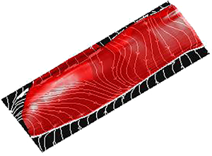
The surface oil flow visualisation after 1.5 h of wind tunnel operation is shown in figure 7(a), and a time lapse of the entire visualisation is available in Movie 1. Boundary layer separation can be inferred from the local accumulation of oil–powder mixture near $x/c=0.20$. Reattachment can be detected where less-pronounced oil accumulation occurs around $x/c=0.45$, followed by a uniform oil distribution downstream in the developing turbulent boundary layer, similar to the results of Selig, Deters & Wiliamson (Reference Selig, Deters and Wiliamson2011). The flow visualisation results agree well with the topology revealed by the limiting streamlines calculated from PIV measurements, with minor variations attributed to experimental uncertainty and unavoidable, minute differences in models and angles of attack settings between the two experiments. A schematic interpretation of the surface oil flow image is presented in figure 7(b), which was constructed with the aid of Movie 1. The revealed LSB topology is analogous to and confirms that inferred from the PIV data. Specifically, a focus of separation (F) can be inferred in the junction region, with a sense of rotation that is consistent with spanwise inflow into the aft portion the LSB. Near the wing tip, no well-defined critical points are found, and a downstream shift in reattachment occurs. These features were also reported in the surface topology sketch based on surface oil flow visualisation of Huang & Lin (Reference Huang and Lin1995) on a cantilevered NACA 0012 wing with $AR=5.0$ at $Re_c=8.0\times 10^4$ and $\alpha =5.0^\circ$, which is reproduced in figure 7(c). The overall similarity between results from different experiments involving different airfoil profiles and flow conditions suggests that the topological changes in the LSB structure near the wing root observed in the present study represent a general LSB topology near a wing root junction.

Figure 7.

(a) Surface oil flow visualisation, present study. Full time lapse in supplementary movie 1 available at https://doi.org/10.1017/jfm.2022.460. (b) Surface topology schematic, present study. (c) Surface topology schematic adapted from Huang & Lin (Reference Huang and Lin1995) on a NACA 0012 wing at $Re_c=8.0\times 10^4$ and $\alpha =5.0^\circ$. Thick lines: separation lines; dashed lines: reattachment lines.

In addition to the surface topology, the wall-normal extent of the LSB is also affected by the wing root junction. The height of the core of the separated shear layer and the thickness of the reverse flow region as measured using the side-view PIV configuration are depicted in figure 8 by the maximum streamwise displacement thickness and maximum height of the $\overline {u}=0$ contour, respectively. The present results from the wing root region are complemented by the wing tip data from Toppings & Yarusevych (Reference Toppings and Yarusevych2021). Both parameters yield similar spanwise trends in the wall-normal extent of the LSB. Near the midspan of the wing, changes in the thickness of the LSB are relatively gradual, and a progressive thickening of the LSB with increasing $z/c$ can be inferred. Approaching the wing root, a local maximum in the bubble height occurs at $z/c=0.35$. At lower $z/c$ locations, the progressive increase in three-dimensional effects is accompanied by a significant reduction in the bubble height. An extrapolation of the rapidly decreasing bubble height for $z/c<0.20$ suggests that the LSB is eventually eliminated by junction effects at a short distance inboard from $z/c=0.10$. Because a reduction in the distance of an inflectionally unstable shear layer from a surface causes a reduction in the growth rates of unstable disturbances (Michalke Reference Michalke1991), substantial changes in the stability and transition process of the separated laminar shear layer are expected to occur near the wing root, which will be explored in § 3.2. Also plotted in figure 8 is the minimum mean streamwise velocity $\overline{u}_{min}/U_\infty$, which indicates the strength of reverse flow within the LSB. Over a majority of the span, the minimum mean streamwise velocity magnitude varies between approximately $5\,\%$ and $10\,\%$ of the freestream velocity, which suggests that the primary instability mechanism is convective in nature. The displacement thickness Reynolds numbers in the present LSB are less than $1000$, for which Alam & Sandham (Reference Alam and Sandham2000) calculated that the reverse flow magnitude required for absolute instability is greater than $15\,\%$ of the freestream velocity. Further, the ratio of the height of the $\overline {u}/U_\infty= 0$ contour to the streamwise displacement thickness in the present LSB is less than $0.56$ at all locations, which is below the threshold of approximately $0.6$ required for absolute instability in the work of Rist & Maucher (Reference Rist and Maucher2002) at comparable Reynolds numbers and reverse flow velocities. Finally, for all spanwise locations, except at $z/c=2.10$, LSB cross sections do not satisfy the criterion proposed by Avanci, Rodríguez & Alves (Reference Avanci, Rodríguez and Alves2019) that requires the inflection point of the velocity profile to be located below the zero-net streamwise mass flux line for absolute instability to occur. Therefore, the primary instability in the junction and midspan regions is expected to be convective in nature. Although the identification of global instability modes is outside the scope of this work, the reverse flow does exceed the threshold required for the stationary global instability identified by Rodríguez & Theofilis (Reference Rodríguez and Theofilis2010), which may be responsible for the spanwise waviness seen in the LSB, similar to that reported by Rodríguez & Gennaro (Reference Rodríguez and Gennaro2019).

Figure 8.

Maximum displacement thickness, maximum height of $\overline {u}/U_\infty =0$ contour and minimum streamwise velocity at each side-view measurement plane. Solid markers: present study; open markers: Toppings & Yarusevych (Reference Toppings and Yarusevych2021); solid line: extrapolation of maximum height of $\overline {u}/U_\infty =0$ contour.

Similar to the trend seen in the junction region, a monotonic decrease in bubble thickness also occurs near the wing tip for $2.00< z/c<2.30$, and at $z/c=2.00$ the bubble thickness reaches a local maximum. This suggests that both types of end conditions cause the thickness of the reverse flow region and height of the separated shear layer to increase near the open ends of the LSB, prior to the onset of the reduction in bubble thickness induced by the end conditions.

The three-dimensional structure of the time-averaged LSB near the wing root is depicted in figure 9, which presents the separation streamsurface in red and the limiting streamlines on the surface of the wing in white. The separation streamsurface is defined as the surface formed from the set of streamlines that emanate from the separation line. The separation streamsurface was calculated using linear interpolation of the stereo-PIV velocity data and streamline integration using the fourth-order Runge–Kutta method. The figure shows that the streamwise extent of the LSB shortens notably in the junction region for $z/c\leq 0.20$, where the separation surface is swept into the recirculation region in the aft part of the LSB by spanwise flow (figure 5b), and the reattachment line shifts upstream. At the same time, for $z/c>0.20$, the mean LSB structure features relatively small spanwise undulations in the locations of separation and reattachment. Similar spanwise variations in mean LSB characteristics have been also reported for nominally two-dimensional flow configurations (Rodríguez & Theofilis Reference Rodríguez and Theofilis2010; Kurelek et al. Reference Kurelek, Tuna, Yarusevych and Kotsonis2021).

Figure 9.

Three-dimensional mean LSB structure near the wing root. Red surface: separation streamsurface; thin lines: limiting streamlines; thick solid line: separation line; thick dashed line: reattachment line.

The foregoing analysis of flow visualisation results and velocity measurements suggests that the LSB on the wing is an open bubble that contains substantial spanwise flow of varying magnitude near the wing root (figure 5b) and tip (Toppings & Yarusevych Reference Toppings and Yarusevych2021, figure 9). Note that the presence of a three-dimensional reattachment line at a given $z$ location does not preclude the exchange of fluid between the recirculation region of a three-dimensional separation bubble and the surrounding flow at that location, as elaborated on by Kremheller & Fasel (Reference Kremheller and Fasel2010) and Toppings & Yarusevych (Reference Toppings and Yarusevych2021). Further insight into the three-dimensional mean LSB flowfield is provided by figure 10, which plots the spanwise volume flow rate ($\overline {\dot {V}}$) through the area ($A$) enclosed by the zero-net streamwise mass flux line (Horton Reference Horton1968) (figure 10 inset) at each side-view PIV measurement plane. Because the spanwise volume flow rate is a function of the LSB cross-sectional area, which also varies along the span of the wing, the mean spanwise velocity ($\overline {\dot {V}}/A$) is also presented in the figure. Estimates near the wing tip are obtained using data from Toppings & Yarusevych (Reference Toppings and Yarusevych2021).

Figure 10.

Spanwise volume flux (black) and mean spanwise velocity (blue) through area enclosed by zero-net streamwise mass flux line. Solid markers: present study; open markers: Toppings & Yarusevych (Reference Toppings and Yarusevych2021).

In the junction region, the inflow of fluid into the recirculation region leads to a positive spanwise volume flow rate, consistent with the positive spanwise velocity contours in the aft portion of the LSB near the wing root in figure 5(b). The largest spanwise volume flow rate is reached at $z/c=0.20$, with the subsequent decrease seen towards the midspan. For $0.4\leq z/c\leq 0.85$, the spanwise volume flux within the LSB is nearly zero, as expected given the similarity between the LSB on the wing and a two-dimensional LSB in this region (figure 4). Near the midspan ($z/c=1.25$), a negative spanwise volume flow rate develops inside the LSB due to the spanwise pressure gradient induced by the tip effects (figure 3b). As the spanwise pressure gradient intensifies towards the wing tip, an increasingly negative spanwise volume flow rate develops, peaking at $z/c=2.10$, before diminishing to zero as the LSB becomes thinner near the wing tip (figure 8). The mean spanwise velocity within the LSB displays a similar spanwise distribution to that of the mean spanwise volume flow rate. This suggests that the observed changes in the spanwise volume flow rate are linked to changes in both LSB cross-sectional area and spanwise velocity, which can be confirmed by comparing figures 5 and 10. The occurrence of local maxima in the magnitude of the mean spanwise volume flow rate and mean spanwise velocity near both the wing root and tip point to a similar mean LSB structure at both types of end conditions.

3.2. Separation bubble dynamics near the wing root

The inherent relation between the separated shear layer dynamics and mean bubble topology suggests that the notable changes observed in the latter near the wing root are accompanied by substantial changes to the former. This is illustrated in figure 11, which presents contours of instantaneous spanwise vorticity (figures 11(a) and 11(b)), and phase-averaged vorticity (figure 11c) at an arbitrary but constant phase across the four side-view measurement planes closest to the wing root. For $z/c\geq 0.15$, the snapshots from the natural and weakly excited flows depict the development of spanwise vortices in the shear layer, which is typical of two-dimensional LSBs (e.g. Häggmark et al. Reference Häggmark, Bakchinov and Alfredsson2000; Hain, Kähler & Radespiel Reference Hain, Kähler and Radespiel2009) and of the present LSB at the planes outside of the junction and tip affected regions. With decreasing $z/c$, the separated shear layer moves closer to the wing surface, as the LSB becomes thinner under the influence of the wing root junction. At $z/c=0.10$, roll-up of the shear layer occurs farther upstream. The earlier formation of vortical structures at $z/c=0.10$ is indicative of earlier transition and consistent with the upstream shift in mean reattachment at this spanwise location (figure 6a). In addition, at $z/c=0.10$, the shed vortices lose coherence more rapidly as they break down to turbulence, which leads to the absence of well-defined vortices in the phase-averaged results at $z/c=0.10$ (figure 11c). This is attributed to the more pronounced influence of three-dimensional junction effects near the wing root, where disturbances are introduced from the turbulent test section wall boundary layer, and where strong mean spanwise flow is present in the aft portion of the LSB (figure 5b). It is of interest to note that the LSB dynamics in the junction region differs from that reported near the wing tip, where a progressive reduction in the strength of the shear layer vortices and delay in transition take place (Toppings & Yarusevych Reference Toppings and Yarusevych2021, figures 17 and 18).

Figure 11.

Spanwise vorticity contours at the four side-view planes closest to the wing root: (a) uncorrelated snapshots from natural flow, (b) phase-locked snapshots from weakly excited flow and (c) phase average from weakly excited flow.

The spanwise velocity measurements corresponding to the results presented in figure 11 are explored in figure 12. The instantaneous snapshots (figures 12(a) and 12(b)) reveal that substantial spanwise velocity fluctuations occur during shear layer vortex formation and breakdown in the aft portion of the LSB. Because the phase-averaged results in figure 12(c) display relatively lower spanwise velocity magnitudes than the instantaneous snapshots, it can be concluded that the strongest velocity fluctuations in the aft portion of the LSB are associated with random vortex deformations and breakdown. Comparing the results from the plane at $z/c=0.10$ with the planes farther from the wing root, it is apparent that stronger spanwise velocity fluctuations occur farther upstream at $z/c=0.10$. This suggests that the more rapid vortex breakdown seen at $z/c=0.10$ (figure 11) is caused by an earlier onset of three-dimensional vortex deformations, likely linked to substantial mean spanwise flow in the junction region (figure 5b).

Figure 12.

Spanwise velocity contours at the four side-view planes closest to the wing root: (a) uncorrelated snapshots from natural flow, (b) phase-locked snapshots from weakly excited flow and (c) phase average from weakly excited flow.

The streamwise growth of velocity fluctuations in the LSB is explored in figure 13, which presents contours of turbulent kinetic energy (TKE) at $y=\delta ^*_x$. The streamwise location of maximum streamwise displacement thickness is shown by the stars, which provide an indication of the mean transition location. Downstream of the maximum streamwise displacement thickness, a substantial increase in TKE occurs due to the shedding of coherent structures (figure 11) and their subsequent breakdown to turbulence. The spanwise variations in the streamwise locations of separation and reattachment are similar to the variations in the location of maximum streamwise displacement thickness and the contours of TKE. In the junction region, the upstream shift in reattachment at $z/c=0.10$ is accompanied by an earlier initial growth of velocity fluctuations, implying that the transition process is substantially influenced by end effects in the junction region.

Figure 13.

(a) Contours of TKE at $y=\delta ^*_x$. Thick solid line: separation line; thick dashed line: reattachment line; thin solid lines: uncertainty in separation and reattachment lines; stars: streamwise location of maximum $\delta ^*$. (b)–(d) RMS fluctuating velocity components at $y=\delta ^*_x$. Shaded area indicates typical uncertainty.

Figures 13(b)–13(d) present the growth of each of the three components of velocity fluctuations along $y=\delta ^*_x$ for the four stereo-PIV measurement planes closest to the wing root. The results reveal that the earlier growth in TKE at $z/c=0.10$ is the result of earlier growth in all three fluctuating velocity components, occurring at comparable initial growth rates to the planes farther from the wing root. The exponential growth of wall-normal velocity fluctuations in the streamwise direction is consistent with that expected from a linear convective instability mechanism. The similarity in the growth rates between the four planes suggests that the primary instability mode is not affected significantly in the junction region. Instead, the earlier appearance of more significant velocity fluctuations in the separated shear layer is likely the result of an increase in the initial amplitude of perturbations. This is substantiated by the streamwise velocity fluctuations in figure 13(b), which indicate that the largest amplitudes in the forward part of the LSB occur at $z/c=0.10$. Thus, although the test section wall turbulent boundary layer is relatively thin (figure 2), its presence introduces higher-amplitude perturbations away from the root, leading to the earlier appearance of significant streamwise and wall-normal shear layer fluctuations (figures 13(b) and 13(c)) at $z/c=0.10$ and earlier shear layer roll-up. Note that, in contrast to the streamwise fluctuations (figure 13b) which saturate at similar amplitudes along the span, the maximum amplitude of wall-normal velocity fluctuations is reduced at the two planes closest to the wing root ($z/c=0.10$ and $0.15$, figure 13c). Here, the closer proximity of the separated shear layer to the wing surface near the wing root (figure 8) is expected to limit the maximum amplitude of wall-normal velocity fluctuations in the junction region. Because the wall-normal velocity fluctuations that occur near reattachment are related to the passage of spanwise shear layer vortices, the reduction in wall-normal velocity fluctuations near the wing root also points to a change in the vortex shedding dynamics in the junction region. This is also highlighted by the significantly earlier onset of spanwise velocity fluctuations at $z/c=0.10$, consistent with the earlier breakdown of the rollers seen in figure 11 at this plane.

The development of shear layer vortices shed from the LSB across the wingspan is investigated further using the top-view PIV configuration. Instantaneous top-view snapshots of streamwise velocity for the natural and weakly excited flows are presented in figure 14. As the top-view light sheet was positioned to intersect the top halves of the shear layer vortices, the spanwise bands of increased streamwise velocity seen in the figure identify the location of the vortices. The vortical structures seen in both the natural (figure 14a) and weakly excited flows (figure 14b) share similar features, although vortices appear to persist slightly farther downstream in the weakly excited flow. Up to the location of mean transition ($X/c\approx 0.40$), the vortices are strongly uniform along the span for $z/c\gtrsim 0.20$. However, farther downstream, the dominant structures rapidly lose spanwise coherence as they undergo three-dimensional deformations. Within the junction region ($z/c\leq 0.20$), shear layer vortices become progressively difficult to identify.

Figure 14.

Instantaneous snapshots of streamwise velocity from top-view PIV.

Proper orthogonal decomposition (POD) was performed on the streamwise velocity fluctuations measured using the top-view PIV configuration based on the method of snapshots (Sirovich Reference Sirovich1987) to obtain a statistical description of spanwise vortex development in the LSB. The energy of the first $20$ POD modes for the natural and weakly excited flows is plotted in figure 15(a) in terms of the spatially averaged TKE of each mode. The two most energetic modes of the natural and weakly excited flows contain substantially more energy than the higher modes and display similar spatial distributions that are offset in the streamwise direction by $1/4$ of the fundamental wavelength, which is indicative of mode pairing. Thus, the first mode pair describes the convection of dominant coherent structures in the aft portion of the LSB (e.g. Ben Chiekh et al. Reference Ben Chiekh, Michard, Grosjean and Béra2004; Lengani et al. Reference Lengani, Simoni, Ubaldi and Zunino2014). For brevity, the spatial distribution of only the most energetic mode is presented in figures 15(b) and 15(c) for the natural and weakly excited flows, respectively. The spatial mode contours reveal similar spanwise vortex development in both the natural and weakly excited flows. Although the weak excitation leads to shed vortices persisting farther downstream of the LSB, the shape and spanwise extent of the spatial mode remains similar, confirming the decay in the modal magnitude for $z/c<0.20$, and indicating a notable deformation of the vortex cores between $z/c=0.1$ and $z/c=0.2$, which is more pronounced in figure 15(c). However, because similar vortex undulations have also been observed in two-dimensional LSBs (e.g. McAuliffe & Yaras Reference McAuliffe and Yaras2005; Kurelek et al. Reference Kurelek, Tuna, Yarusevych and Kotsonis2021), this cannot be conclusively attributed to end effects.

Figure 15.

(a) POD modal energy of streamwise velocity fluctuations from top-view PIV. (b), (c) Dominant spatial POD modes for natural and weakly excited flow.

A statistical comparison of vortex development at different spanwise locations is facilitated using POD of the velocity data from each side-view measurement plane in the natural flow, also obtained using the method of snapshots. Figure 16 presents the spatially averaged TKE of the 20 most energetic modes at each plane, enabling a comparison of modal energy between measurement planes. The similar energy content of the first two modes at each plane is indicative of mode pairing. This was verified by inspection of the spatial mode shapes. The fluctuations in the relative energy content of the most energetic mode pair along the span correlates with the spanwise changes in the mean reattachment point (figure 6) and TKE (figure 13a), linked to the changes in the shear layer roll-up location. Specifically, the earlier roll-up and transition, which lead to the upstream advancement of reattachment and earlier TKE saturation, is associated with greater energy of the dominant mode pair in figure 16. Consistently, a notable increase in the energy of the two most energetic modes occurs at the plane closest to the wing root, where earlier shear layer shedding takes place.

Figure 16.

Spatially averaged TKE of the first 20 POD modes at each side-view measurement plane.

Figure 17 depicts the streamwise, wall-normal and spanwise components of the first POD mode for the four planes closest to the wing root. The second mode is also shown for $z/c=0.25$ to illustrate the spatial topologies of the paired first and second modes, which is typical of the other planes shown. Note that the spatial modes are multiplied by $\sqrt {\langle TKE\rangle }$, which allows for a direct comparison of modal velocity fluctuation magnitudes between planes. At all planes, a streamwise periodic pattern is seen in the aft portion of the bubble. At $z/c=0.25$, which is representative of the planes farther from the wing root, the $x$ and $y$ components of $\varPhi ^{(1)}$ and $\varPhi ^{(2)}$ are typical of those obtained from PIV measurements of two-dimensional LSBs (e.g. Lengani et al. Reference Lengani, Simoni, Ubaldi and Zunino2014; Kurelek et al. Reference Kurelek, Yarusevych and Kotsonis2019) and correspond to spanwise vortices shed from the separated shear layer (figure 11), which produce strong streamwise and wall-normal velocity fluctuations. The spanwise modal velocity fluctuations are attributed to the consistent occurrence of three-dimensional vortex deformations at constant spanwise locations, similar to those observed in two-dimensional LSBs (e.g. Kurelek et al. Reference Kurelek, Tuna, Yarusevych and Kotsonis2021). In the junction region ($z/c \leq 0.20$), the magnitudes of the wall-normal velocity fluctuations of the first POD mode progressively diminish as the wing root is approached, consistent with the reduction in the maximum amplitude of wall-normal RMS velocity fluctuations (figure 13c). In addition, an increase in the magnitudes of the spanwise component of the modes occurs near the wing root, most prominently at $z/c=0.10$ (figure 17a), substantiating the previous observation that an increase in the level of spanwise velocity fluctuations occurs near the wing root. There is also a notable change in the modal shape components, with streamwise mode shape at $z/c=0.10$ becoming similar to wall-normal mode shapes seen farther outboard. The observed changes in the first mode shape topologies and magnitudes suggest that vortex core reorientation occurs in the junction region. The spatial correlation between opposite signs of streamwise ($\varPhi _u^{(1)}$) and spanwise ($\varPhi _w^{(1)}$) components at $z/c = 0.10$ (figure 17a) suggests that the vortex cores tilt into the negative $y$ direction in the junction region, which is consistent with the reduction in height of the LSB in the junction region.

Figure 17.

Spatial distribution of selected POD modes at the four planes nearest to the wing root. The shaded area has been excluded from the POD due to high uncertainty in the thin upstream boundary layer.

A comparison of the phase-averaged vortex shedding obtained from the top and side views is presented in figure 18. Figure 18(a) presents contours of phase-averaged streamwise velocity ($\tilde {u}$) from the top view, whereas figure 18(b) presents contours of $\lambda _2$ criterion (Jeong & Hussain Reference Jeong and Hussain1995) obtained from the volumetric reconstruction of side-view measurement planes at the same phase angle. The full cycle sequence of figure 18(a) is available in Movie 2. Consistent with the instantaneous snapshots (figure 14) and POD results (figure 15), the phase-averaged results reveal largely two-dimensional periodic vortex shedding outside of the junction region. This confirms the association between the bands of high streamwise velocity in the top-view measurements with the vortices observed in the side-view planes. Within the junction region ($z/c\leq 0.20$), identification of vortices becomes progressively more difficult. The absence of clearly defined phase-averaged vortices near $z/c=0.10$ in both figures 18(a) and 18(b) is attributed to significant cycle-to-cycle variations in the shedding process that result in phase smearing.

Figure 18.

(a) Phase-averaged streamwise velocity contours from top-view PIV of weakly excited flow. Full cycle sequence available in Movie 2. (b) Isosurfaces of $\lambda _2$ reconstructed from side-view phase-averaged PIV of weakly excited flow. Grey: $\lambda _2 c^2/U_\infty ^2=-100$, red: $\lambda _2c^2/U_\infty ^2=-500$.

To better understand the changes in vortex shedding across the span, vortex identification was employed. Vortex core locations were defined as local minima of $\lambda _2$ criterion with a minimum prominence of $1500U_\infty ^2/c^2$. Figure 19(a) presents the locations of all vortex cores identified in the four planes closest to the wing root in the natural flow case. At all planes, the identified vortex cores are clustered around the streamwise displacement thickness (dashed line) in the aft portion of the LSB, illustrating that the roll-up occurs primarily in the vicinity of the maximum bubble height location. The reduction in LSB thickness in the junction region (figure 8) causes a decrease in the wall normal distance of vortex cores from the wing surface. Consistent with the earlier growth of velocity fluctuations closer to the wing root (figure 13), vortices form progressively farther upstream for $z/c\leq 0.15$ compared with the planes closer to the midspan. In addition, the variability of vortex core locations in the wall-normal direction increases notably in the same region.

Figure 19.

(a) Locations of identified vortex cores at selected planes. Dashed line: $\delta ^*_x$. (b) Mean wall-normal vortex core position within a window of $0.01c$ of the $x$ location of maximum $\delta ^*_x$. Solid markers: present study; open markers: Toppings & Yarusevych (Reference Toppings and Yarusevych2021).

The mean wall-normal vortex core location at the $x$ location of maximum streamwise displacement thickness is plotted in figure 19(b) for the entire span of the wing based on the data from the present study and that from Toppings & Yarusevych (Reference Toppings and Yarusevych2021) near the wing tip. The error bars indicate one standard deviation of the wall-normal vortex core locations. Comparing figures 8 and 19(b), it is apparent that the distance of the vortex cores from the wing surface displays similar trends to the LSB thickness. Near the midspan of the wing, the wall-normal distance of the vortex cores is relatively uniform between the local maxima that occur at $z/c=0.35$ and $1.90$. At the wing root and tip, a reduction in wall-normal vortex core distance is observed. The substantial decrease in wall-normal vortex core location in the junction region provides further evidence for vortex core tilting towards the wing surface.

The frequency content of velocity fluctuations in the LSB was investigated using the high-speed top-view PIV configuration in the natural flow. Figure 20 presents the variation of power spectral density of streamwise velocity fluctuations across the span. The spectral analysis was performed using Welch's method with a window size of $2^7$ samples. The spectra presented were obtained by averaging the power spectral density over $0.35\leq x/c\leq 0.5$ at each $z$ location, i.e. within the region where prominent vortex shedding is observed. The resulting uncertainty in power spectral density is less than $23\,\%$, and the frequency resolution is $0.3U_\infty /c$. For $z/c>0.20$, spectral energy is concentrated within the band of frequencies in the range $15.6< fc/U_\infty <17.9$. This frequency range is in good agreement with the central shear layer instability frequencies reported for the same wing model and flow conditions in Toppings et al. (Reference Toppings, Kurelek and Yarusevych2021), and is similar to that expected for natural transition in the separated shear layer (e.g. Hain et al. Reference Hain, Kähler and Radespiel2009). Outside of the junction region, the dominant energy content of velocity fluctuations remains centred at $fc/U_\infty \approx 16$, suggesting that the primary instability mode in the midspan region of the wing is largely unmodified by root effects. Although the relative breadth of the spectral content around the central frequency points to cycle-to-cycle variations in the shedding process, the spanwise uniformity of the spectral results indicates that the vortex shedding frequency does not change substantially along the span for $z/c>0.20$. For $z/c<0.20$, a rapid decay of velocity fluctuations around $fc/U_\infty =16$ is seen, with no significant spectral peaks seen at or beyond $z/c\approx 0.15$. This is partly attributed to the deformation and earlier breakdown of vortices in this region, and the decrease in LSB thickness in the junction region which shifts the shear layer closer to the surface and away from the PIV measurement plane.

Figure 20.

Spectral analysis of streamwise velocity fluctuations.

The influence of the wing root junction on the LSB transition dynamics is also seen in the spanwise changes that occur to the streamwise vortex shedding wavelength. Streamwise wavelength spectra of wall-normal ($\widehat {\mathcal {F}_{v'v'}}$) and spanwise ($\widehat {\mathcal {F}_{w'w'}}$) velocity fluctuations from each side-view measurement plane are presented in figures 21(a) and 21(b), respectively. The spectra presented were obtained by averaging the power spectra from each instantaneous velocity field snapshot over $1000$ snapshots obtained at a given $z/c$ plane. The relative uncertainty in the averaged power spectral density is less than $7\,\%$ and the wavelength resolution at a given wavelength ($\lambda$) is equal to $\lambda ^2/(0.125c)$. Each spectrum has been normalised by total energy and shifted by an order of magnitude for clarity. Similar to the frequency analysis from the top view, the wavelength of the spectral peaks in both velocity fluctuation spectra is largely uniform away from the wing root. The mean wavelength of the spectral peaks is $\lambda /c=0.039$, which agrees with the spacing between consecutive vortices in figures 11 and 12. In the junction region ($z/c\leq 0.20$), the reduction in relative magnitude and broadening of the spectral peak of wall-normal fluctuations (figure 21a) is accompanied by an increase in relative magnitude of the spectral peak of spanwise velocity fluctuations (figure 21b) in agreement with the change in the dominant components of coherent velocity fluctuations seen in the POD spatial modes at the planes near the wing root (figure 17) and increase in spanwise velocity fluctuations (figures 11 and 12) attributed to vortex deformations and earlier breakdown. The spectral results also indicate that the fundamental streamwise vortex shedding wavelength increases in the junction region to $\lambda /c=0.060$ at $z/c=0.10$. It is speculated that this change in wavelength may be a result of vortex core reorientation in the junction region. In contrast, measurements near the wing tip do not show evidence of vortex core reorientation or a change in the fundamental wavelength (Toppings & Yarusevych Reference Toppings and Yarusevych2021, figure 24(a)). Therefore, both the mean flow and the vortex dynamics in immediate proximity to the ends of the LSB on a finite wing are affected by the type of end condition imposed.

Figure 21.

Streamwise wavelength spectra. All spectra have been normalised by total energy and each $z/c$ location has been shifted an order of magnitude for clarity. Dashed line: $\lambda /c=0.039$; $x$ markers: maximum normalised power spectral density.

The foregoing discussion of vortex shedding characteristics shows that, similar to the mean LSB structure, shear layer transition and vortex shedding dynamics are largely unaffected by the presence of the wing root outside of the junction region ($z/c>0.20$). In the midspan region of the wing, the transitioning separated shear layer rolls up into largely two-dimensional spanwise vortices near the location of maximum displacement thickness, and spanwise variations in the frequency and wavelength of shear layer vortex shedding are relatively small. Within the junction region ($z/c\leq 0.20$), shear layer transition is affected by the presence of the test section wall boundary layer and spanwise flow, which increases the initial amplitudes of perturbations in the separated laminar shear layer leading to earlier vortex roll-up. Large spanwise velocity magnitudes in the junction region point to vortex deformations and more rapid vortex breakdown, leading to earlier reattachment. As a result of these changes to the LSB dynamics, the streamwise and wall-normal extent of the LSB is substantially reduced near the wing root. This is in contrast to the LSB behaviour near the wing tip, where a delay in vortex roll-up and breakdown causes a lengthening of the reverse flow region (Toppings & Yarusevych Reference Toppings and Yarusevych2021).