


1. Introduction
The motion of particles in a turbulent carrier fluid subject to exogenous body forces manifests in myriad applications such as ash settling (Mingotti & Woods Reference Mingotti and Woods2020), energy production (Ishii Reference Ishii1977; Guet & Ooms Reference Guet and Ooms2006) and bubbly wakes (Carrica et al. Reference Carrica, Drew, Bonetto and Lahey1999). These particles may experience multiphysics including nucleation, coalescence, dissolution and growth, but their dispersion by energetic eddies of the background flow naturally lends itself to the field of turbulence modelling. In the framework of population balance equations, as reviewed in Shiea et al. (Reference Shiea, Buffo, Vanni and Marchisio2020), particles can be segregated into size classes associated with a drift velocity,  $u_d$, relative to the background flow with root-mean-square velocity $u_{rms}$. In nature, $u_d/u_{rms}$ can be large; a Hinze-scale 1 mm bubble, the largest size that should not undergo breakup, may rise at $12\,{\rm cm}\,{\rm s}^{-1}$, while a characteristic upper ocean turbulence velocity is closer to $2\,{\rm cm}\,{\rm s}^{-1}$ (Detsch & Harris Reference Detsch and Harris1989; Deane & Stokes Reference Deane and Stokes2002; D'Asaro Reference D'Asaro2014).
For dilute, low Stokes number ( $St$) particle-laden flows with negligible particle–particle interactions, the particle concentration – or void concentration – fields can be described with the passive scalar advection–diffusion equation (Moraga et al. Reference Moraga, Larreteguy, Drew and Lahey2003). A low $St$ particle flow is one for which the particle momentum relaxation time is far smaller than the flow time scale, and ‘dilute’ flows should have particle volume fractions ( $\phi$) less than ${\sim }O({10^{-3}}$) (Brandt & Coletti Reference Brandt and Coletti2022). Each class can be evolved separately and forces like buoyancy and gravity are accounted for with additional velocity components from relations like the drag law of Schiller & Naumann (Reference Schiller and Naumann1935). For sedimenting particles, this drift is aligned with the gravity vector; in the case of bubbly flows, it is generally anti-parallel.
Solving for full-resolution scalar evolution when only a mean state is required to determine quantities of engineering interest is prohibitively expensive. Averaging to find the mean occurs in homogeneous spatio-temporal dimensions, defined through Reynolds averaging or filtering in the large-eddy simulation context. When averaging is applied to the Navier–Stokes and advection–diffusion equations that govern the evolution of scalar-laden fluid flows, the turbulent scalar flux, given by  $\overline {u_i c}$, appears. Here, $u_i$ and $c$ are the fluctuating velocity and scalar fields, respectively, and $\bar {\bullet }$ is an average. This term represents unresolved scalar transport by turbulence and its closure is essential to making transport simulations tractable.
A common model form for the turbulent scalar flux is gradient diffusion, written analogously to Fickian diffusion as  $\overline {u_i c} = - D_{ij} ({\partial \overline {C}}/{\partial x_j})$, with $D_{ij}$ representing eddy diffusivity and $C$ the full scalar field. Foundational work has shown eddy diffusivity decays with increased drift, but few extant models for capturing the flux are algebraic closed-form expressions (Yudine Reference Yudine1959; Moraga et al. Reference Moraga, Larreteguy, Drew and Lahey2003; Reeks Reference Reeks2021). An exception is Csanady (Reference Csanady1963), which derives an expression for particle diffusivity scaling as a function of $u_d$ from theoretical arguments about the form and relevant parameters of the velocity autocorrelation, but Squires & Eaton (Reference Squires and Eaton1991) showed disparities between it and measured experimental and computational turbulent data.
As Csanady (Reference Csanady1963) serves as a starting point for more complex models (e.g. Wang & Stock Reference Wang and Stock1993) and particle-laden turbulence is still a ripe topic (e.g. Berk & Coletti Reference Berk and Coletti2021), we wish to revisit this problem using the recently developed macroscopic forcing method (MFM) to calculate eddy diffusivity (Mani & Park Reference Mani and Park2021; Shirian & Mani Reference Shirian and Mani2022). In general, the eddy diffusivity is a non-local spatial and temporal operator, but when there is separation of scales between the large-eddy size and the scalar cloud size, as is relevant for this problem, measurement of a single local coefficient of eddy diffusivity, denoted  $D^0$ and sometimes called a dispersion coefficient, suffices. Mani & Park (Reference Mani and Park2021) showed that $D^0$ is the leading-order moment of the full eddy diffusivity operator and Shende & Mani (Reference Shende and Mani2022) used it to predict scalar transport. Furthermore, it is the first term in the Kramers–Moyal approximation of the integro-differential kernel that defines the true eddy diffusivity operator.
In this work, we propose a model using measurements of eddy diffusivity by MFM in numerical simulations of scalar fields driven by homogeneous, isotropic turbulence (HIT) over a range of drift velocities. The MFM has more favourable computational costs when compared with a similar Lagrangian method for this a priori modelling approach. The proposed model better fits empirical data and theoretical constraints for tracers subject to drift.
2. Model problem
Consider a triply periodic cubic domain of HIT. When  $u_d = 0$, the diffusivities along the three principal axes – $D^0_{11}$, $D^0_{22}$ and $D^0_{33}$ – are all equal to $D^0$. If we impose a non-negative drift velocity in the $x_1$ direction, the symmetry of the set-up is broken such that only the diffusivities in the $x_2$ and $x_3$ directions are equal and all are affected by drift. While the derivation herein reaches conclusions similar to others (e.g. Csanady Reference Csanady1963; Squires & Eaton Reference Squires and Eaton1991; Mazzitelli & Lohse Reference Mazzitelli and Lohse2004), we distinctly adopt an Eulerian perspective.
For  $u_d = 0$, we begin with the Lagrangian formulation of eddy diffusivity of Taylor (Reference Taylor1922), with the scalar represented by tracer particles with position $X_i(t)$ and velocity $V_i(t)$. Taylor (Reference Taylor1922) writes the eddy diffusivity in the $x_1$ direction of a ensemble of such particles, in the long time limit. If the velocity field is statistically stationary, this can be expressed as
 \begin{equation} D^0_{11} = \int^\infty_0 \langle (V_1(\tau+t) V_1(t)\rangle\,{\rm d}\tau, \end{equation}
where  $\langle \bullet \rangle$ represents an average over the ensemble and $\tau$ is a temporal offset. In the high Péclet number ( $Pe$) limit, where molecular diffusivity is far smaller than eddy diffusivity, $V_i(t)$ is the flow velocity at a given particle's position. Therefore, we can express the underlying Eulerian velocity field component, $u_1$, as a function of the full three-dimensional tracer position, $\boldsymbol {X}$. This yields
 \begin{equation} D^0_{11} = \int^\infty_0 \langle u_1(\boldsymbol{X}(t),t) u_1(\boldsymbol{X}(t+\tau),t+\tau) \rangle\,{\rm d}\tau. \end{equation}
We define a standard complementary characteristic turbulence length scale as
 \begin{equation} L_{11} = \frac{1}{u^2_{rms}} \int^\infty_0 \langle u_1(x_1, x_2, x_3,t) u_1(x_1+r,x_2,x_3,t) \rangle\,{\rm d}r, \end{equation}
where  $r$ is a spatial offset, $\langle \bullet \rangle$ now represents an average over all independent variables. Here, $u_{rms}$ normalizes the velocity autocorrelation at zero displacement, namely $\sqrt {\langle u_1u_1 \rangle }$.
Classical Brownian motion analysis posits that scalar diffusivity at infinite time scales as  $u_{rms}^2 \tau _k$, where $\tau _k \equiv L_k/u_{rms}$ denotes some time scale of the underlying flow development and $L_k = 2L_{11}$ is the large-eddy length scale. Consider the scalar field now with some constant drift velocity, $u_d$, with respect to the flow: for very small $u_d$, the fundamental turbulence statistics felt by a scalar parcel are not largely affected and the classical model holds. In the opposite limit that $u_{rms} \ll u_d$ such that $L_{11}/u_d \ll \tau _k$, however, this picture is not appropriate.
In this limit, the scalar field transits the turbulence field at a very fast time scale  $\tau _d = L_{11}/u_d$, such that scalar particles drift before the local flow has evolved. The turbulence can therefore be considered frozen compared to the evolution of the scalar field for computing (2.2), and a leading-order approximation for the differential translation of a scalar parcel is $\Delta X_1 = {\rm d}r \approx u_d\,{\rm d}t$. Thus, the addition of a very large drift is equivalent to examining a translating inertial coordinate frame with respect to the frozen flow, akin to Taylor's hypothesis. These premises allow us, for very large $u_d$, to rewrite (2.2) as
 \begin{equation} \lim_{u_d \to \infty} D^0_{11} = \int^\infty_0 \langle u_1(x_1, x_2, x_3,t) u_1(x_1+u_d\tau,x_2,x_3,t) \rangle\,{\rm d}\tau. \end{equation}
 We have here posited that the change in particle position is purely due to drift, and over the time of  $O(L_{11}/u_d) \ll \tau _k$ where the kernel is non-zero, the field $u_1$ does not change. If we now use a change of variable between the displacement and the drift velocity, we can write
 \begin{equation} \lim_{u_d \to \infty} D^0_{11} = \int^\infty_0 \langle u_1(x_1, x_2, x_3,t) u_1(x_1+r,x_2,x_3,t) \rangle d(r/u_d) = u^2_{rms} \frac{L_{11}}{u_d}. \end{equation}
Here,  $L_{11}$ is the correlation length scale in (2.3) and it requires the spatial correlation drop to zero in the domain. For the transverse diffusivities, $D^0_{22} = D^0_{33}$. We can therefore similarly write
 \begin{equation} \lim_{u_d \to \infty} D^0_{22} = \int^\infty_0 \langle u_2(x_1, x_2, x_3,t) u_2(x_1+r,x_2,x_3,t) \rangle d(r/u_d) = u^2_{rms} \frac{L_{22}}{u_d}. \end{equation}
Appealing to the isotropy of the underlying velocity fields, we also can show that
 \begin{equation} \lim_{u_d \to \infty} D^0_{22} = \int^\infty_0 \langle u_1(x_1, x_2, x_3,t) u_1(x_1,x_2+r,x_3,t) \rangle d(r/u_d) = u^2_{rms} \frac{L_{22}}{u_d}. \end{equation}
 This asymptotic limit jibes with intuition, as a particle with infinite  $u_d$ samples zero mean velocity over every time horizon in homogeneous turbulence. This decay of $D^0_{ii}$ with increasing $u_d/u_{rms}$, the ‘crossing trajectories’ effect of Yudine (Reference Yudine1959) and Csanady (Reference Csanady1963), persists in relatively high Reynolds number ( $Re$) bubble experiments (Mathai et al. Reference Mathai, Huisman, Sun, Lohse and Bourgoin2018).
We seek a model form that analytically matches the exact behaviour at the infinite and zero drift velocity limits. In the intermediate regime, the model should be a smooth and monotonic function of the drift velocity, so a simple model form that captures the asymptotic limits of infinite and zero drift is
 \begin{equation} \frac{D^0_{ii}}{D^0} \approx \Bigg( 1 + \left(\frac{u_dD^0}{L_{ii}u^2_{rms}}\right)^{\alpha_{ii}} \Bigg)^{{-}1/\alpha_{ii}} = \left( 1 + \left(\frac{u_d}{u^*_{ii}}\right)^{\alpha_{ii}} \right)^{{-}1/\alpha_{ii}}. \end{equation}
Here,  $\alpha _{ii}$ is a free parameter and $u_{ii}^*$ is an Eulerian ‘diffusion velocity’ that competes with the drift and is defined using Eulerian measures as
 \begin{equation} u^*_{ii} = \frac{u^2_{rms} L_{ii}}{D^0}. \end{equation}
 In incompressible flows,  $L_{22} = L_{33} = L_{11}/2$ (Csanady Reference Csanady1963). The eddy diffusivity at large drift velocity can be written as $D^0_{ii}/D^0 = u^*_{ii}/u_d$. In contrast, Csanady (Reference Csanady1963) proposed
 \begin{equation} \frac{D^0_{ii}}{D^0} \approx \Bigg( 1 + \left(\frac{\gamma_{ii}~\beta~ u_d}{u_{rms}}\right)^2 \Bigg)^{{-}1/2}, \end{equation}
where  $\beta$ is defined with Lagrangian and Eulerian statistics and $\gamma _{22} = 2\gamma _{11} = 2$.
The proposed model form of (2.8) is very similar to (2.10), suggesting the space of candidate functions appropriate for this problem is narrow. As the adopted problem set-up (i.e. one-way coupled, dilute particle limit, negligible inertial effects) is a simplification, even such an approximate model should offer substantial predictive value.
3. Numerical set-up
Direct numerical simulation (DNS) of forced incompressible HIT in a triply periodic box of edge length  $L_{box}$ provides the data for this test. Solved with continuity are the incompressible Navier–Stokes momentum equations with a linear forcing term. They are written as
 \begin{equation} \frac{\partial{u_i}}{\partial{t}} + \frac{\partial{u_i u_j}}{\partial x_j} ={-} \frac{1}{\rho} \frac{\partial p}{\partial x_i} + \nu \frac{\partial^2 u_i}{\partial x_j \partial x_j} + A\widetilde{u_i}, \end{equation}
where  $A$ is a controller that maintains the turbulent kinetic energy, $k \equiv u_i u_i/2$, at a prescribed level, $\rho$ is the fluid density and $\nu$ is the kinematic viscosity. This approach is similar to Bassenne et al. (Reference Bassenne, Urzay, Park and Moin2016), but with a high-pass filtered velocity described in spectral space as $\widehat {\widetilde {u_i}} = G({|\boldsymbol {{k}}|})\widehat {u_i}$, where $|\boldsymbol {k}|$ is the wavenumber magnitude and
 \begin{equation} G({|\boldsymbol{k}|}) = \begin{cases} 0, & {|\boldsymbol{k}|} \leq 2, \\ \dfrac{1}{2} - \dfrac{1}{2}\cos({\rm \pi} ({|\boldsymbol{k}|}-2)), & 2 < {|\boldsymbol{k}|} \leq 3,\\ 1, & {|\boldsymbol{k}|} > 3. \end{cases} \end{equation}
 In figure 1, plotted instantaneous energy spectra show decay at the largest scales for all considered  $Re$. The values of $L_k$, $L_{11}$, $L_{22}$ and $L_{33}$ are all less than $L_{box}/2$ by construction due to the filtered energy injection. As such, the simulations are not influenced by the cubic box shape or orientation, unlike the standard linear forcing method, as in Rosales & Meneveau (Reference Rosales and Meneveau2005).

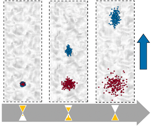
Figure 1. Instantaneous unnormalized velocity autocorrelations (a) and normalized energy spectra  $E(kL_{11})/u_{rms}^2L_{11}$ (b) for the cases in a $2{\rm \pi} ^3$ box, with filtered forcing preventing energy growth in the largest modes. Note that $u_{rms} = 1$ for all cases.
To quantify eddy diffusivity, the MFM formulation of Mani & Park (Reference Mani and Park2021) is used with code adapted from Pouransari, Mortazavi & Mani (Reference Pouransari, Mortazavi and Mani2016) for solving the governing equations on a staggered  $N^3$ grid with finite volume operators and a Runge–Kutta time-advancement scheme. The MFM measures the response of the scalar field to an imposed macroscopic forcing by solving an additional equation for a scalar field with molecular diffusivity $D_m$. Following the procedure of Shirian & Mani (Reference Shirian and Mani2022) for finding $D^0$, we decompose the scalar field as $C = \overline {C} + c$ and add a macroscopic source term, $s$, to the scalar equation so that $c$ is governed by
 \begin{equation} \frac{\partial{c}}{\partial{t}} + \boldsymbol{\nabla} \boldsymbol{\cdot} \left( ( \boldsymbol{u} + \boldsymbol{u}_d ) c \right) = D_m \nabla^2 c - (\boldsymbol{u} + \boldsymbol{u}_d ) \boldsymbol{\cdot} \boldsymbol{\nabla} \overline{C} + s(\boldsymbol{x},t). \end{equation}
 Following the method of moments, the forcing maintains  ${\partial \overline{C}}/{\partial x_i} = 1$ (Mani & Park Reference Mani and Park2021). Setting $i = 1$ allows measurement of the axial diffusivity in the direction of drift and $i = 2, 3$ allows quantification of transverse diffusivity in directions perpendicular to drift. Table 1 summarizes parameters swept to measure eddy diffusivity in the $x_1$ and $x_2$ directions.
Table 1. Summary of measured values relevant for the computation of  $D^0_{11}$ and $D^0_{22}$.

In all cases,  $\nu =D_m$ and $u_{rms} = \sqrt {2k/3} = 1$. The underlying field being HIT means the root-mean-square value for each of the three velocity components is this $u_{rms}$. Once the velocity and scalar fields are fully developed, $D^0_{ii} = -\overline {u_ic}$ is post-processed from the turbulent scalar flux for a time of $O(200\unicode{x2013}500)\tau _k$. Confidence intervals are calculated using the standard error of each mean statistic by constructing decorrelated samples of appropriate length compared with $\tau _k$ (Shirian, Horwitz & Mani Reference Shirian, Horwitz and Mani2023). For each simulation, $\varDelta /\eta = \varDelta /\lambda _B \lessapprox 2.1$, where $\varDelta$ is the grid spacing, $\eta \equiv \nu ^{3/4}\epsilon ^{-1/4}$ is the Kolmogorov length scale, $\lambda _B$ is the Batchelor scale and $\epsilon$ is the energy dissipation rate. We also report $Re_\lambda \equiv \sqrt {{15 u^4_{rms}}/{\epsilon \nu }}$. This resolution, which can also be reported as $k_{max}\eta \gtrapprox 1.5$, where $k_{max}$ is the maximum resolved flow wavenumber, is sufficient to resolve the low-order statistics studied herein and in line with canonical guidelines (Pope Reference Pope2000), studies of flow energetics (Kaneda et al. Reference Kaneda, Ishihara, Yokokawa, Itakura and Uno2003; Bassenne et al. Reference Bassenne, Urzay, Park and Moin2016) and other works studying particle diffusivity (Squires & Eaton Reference Squires and Eaton1991; Mazzitelli & Lohse Reference Mazzitelli and Lohse2004; Jung, Yeo & Lee Reference Jung, Yeo and Lee2008).
3.1. Comparison of MFM with Lagrangian formulae
We show equivalence in the MFM and Lagrangian definitions of eddy diffusivity. The MFM measures  $D^0$ by calculating the correlation of simulated scalar and velocity fields. The Eulerian–Lagrangian method (ELM), in contrast, simulates scalar particles in a background flow to calculate (2.1). Following Falkovich, Gawędzki & Vergassola (Reference Falkovich, Gawędzki and Vergassola2001), the inertialess scalar particles are governed by ${\rm d}\boldsymbol {X} = (\boldsymbol {u}(t) + \boldsymbol {u_d})\,{\rm d}t + \sqrt {2D_m}\,{\rm d}\boldsymbol {W}$. Here, $\boldsymbol {W}(t)$ is a zero-mean, unity-variance Weiner process that allows this Langevin equation to correspond to the advection–diffusion equation solved by MFM.
To assess this equivalence, both methods measure eddy diffusivity from the same HIT case of  $L_{box} = 2{\rm \pi}$ and $Re_\lambda = 14.4$ from table 1 with $u_d = 0$. In addition to the Eulerian DNS, MFM requires solution of (3.3) on $O(10^5)$ mesh points. The ELM requires the same flow-field DNS, along with Lagrangian trajectory simulations for $O(10^6)$ particles. Interpolation of velocity to particle locations uses modified Akima piecewise cubic Hermite functions.
For the candidate turbulent flow, figure 2 compares the measured estimate of the mean value of the eddy diffusivity as a function of the number of ensembles considered. Each independent ensemble is of length  $\approx 10 \tau _k$, collected from a fully developed DNS. The mean estimate from both methods is approximately the same for this realization, but the confidence intervals are quite dissimilar in their size. The MFM provides more confident mean estimates for this application and is more scalable for simulations, as Eulerian fields are easier to distribute and solve with parallel computing than Lagrangian particles. An additional advantage of MFM not utilized here is that MFM can find higher non-local moments of the diffusivity kernel beyond the local-limit leading-order moment (Mani & Park Reference Mani and Park2021).

Figure 2. Mean estimates of  $D^0$ for the $Re_\lambda =14.4$ case using MFM and ELM with 95 % confidence intervals showing convergence to the final estimate from each method (– –).
4. Results and discussion
Equation (2.8) is fitted to the mean diffusivity data from the cases of table 1 as a function of  $u_d$. An iterative method is used to determine $\alpha _{11}$ and $\alpha _{22}$ and the forthcoming section will show that the value of $\alpha _{ii}$ is largely invariant to the tested Reynolds numbers.
In figure 3,  $D^0_{11}$ and $D^0_{22}$ values are plotted for the $Re_\lambda = 14.4$ cases as a function of drift. The eddy diffusivity decay trends for the two directions differ for three values of $L_{box}$. At low drift velocities, the model accurately describes the data; however, at high drift, the $2{\rm \pi} ^3$ box data diverge from the analytic scaling. For a fixed box size, the computational value of $D^0_{ii}$ asymptotes to a non-zero value in the limit of large drift velocity, in violation of the analytical derivation presented earlier. This effect can be explained: in a finite periodic domain, a large drift velocity, $u_d > L_{box}/\tau _k$, subjects a scalar particle to see the same turbulence field in a characteristic advection time. Therefore, the autocorrelation becomes non-zero and the diffusivity value saturates. Figure 3 shows that increasing the computational domain size ameliorates this effect and improves data convergence to the model prediction for the highest drift velocities studied. This effect, however, has minimal effect on parameter choice: for further details, see Appendix B.

Figure 3. Convergence of  $D^0_{11}$ and $D^0_{22}$ with respect to box size for $Re_\lambda = 14.4$. Dashed lines represent (2.8) for $\alpha _{11} = 3.9$ (a,b) and $\alpha _{22} = 1.9$ (c,d). Certain MFM data are shown with representative 95 % confidence intervals, which consider only the statistical error and exclude finite box-size error; arrows indicate convergence with increasing box size. Panels (a,c) show standard axes, while panels (b,d) show log–log axes. The data and Appendix B suggest criteria for which the box size of $2{\rm \pi}$ is sufficient.
We now examine the effect of  $Re$. In figure 4, $D^0_{11}$ and $D^0_{22}$ at three $Re_\lambda$ values for $u_d/u_{rms} < 5$ are shown and the data collapse when normalized by $u^*_{ii}/u_{rms}$. There is good agreement between the computational data and model predictions over the drift velocities and Reynolds numbers explored for $\alpha _{11} \approx 4$ and $\alpha _{22} \approx 2$, based on the values from figure 3. Since $\alpha _{22} = 2$ is used in the literature and Appendix C suggests that $\alpha _{11} \leq 4$, we adopt the closest integer approximations of $\alpha _{11} = 4$ and $\alpha _{22} = 2$ for figure 4 and the remainder of this work. This observed agreement is better and has narrower scatter about the model prediction than presented in Squires & Eaton (Reference Squires and Eaton1991), where $\alpha _{11}=\alpha _{22}=2$. This may be due to the long simulation time and Eulerian MFM method for quantification of $D^0_{ii}$.

Figure 4. The MFM-measured  $D^0_{11}$ and $D^0_{22}$ as a function of $u_d/u^*_{ii}$ for different flow Reynolds numbers for $L_{box} = 2{\rm \pi}$. The dashed lines represent the analytical curve given by (2.8) for $\alpha _{11} = 4$ (top) and $\alpha _{22} = 2$ (bottom). Certain MFM data are shown with representative 95 % confidence intervals, which consider only the statistical error and exclude finite box-size error. Panel (a) shows standard axes, while panel (b) shows log–log axes.
Absent drift, Shirian & Mani (Reference Shirian and Mani2022) used MFM to similarly show that scale-dependent eddy diffusivity, normalized by  $u_{rms}$ and an eddy length scale, was largely invariant to $Re$. When considering $\overline {u_ic}$, this should not be surprising, as taking an average of a multi-scale field that decays rapidly in magnitude at large wavenumbers ensures that the large-scale content dominates. Bos, Touil & Bertoglio (Reference Bos, Touil and Bertoglio2005), for example, show that even at $Re_\lambda = 28$, a relatively sharp scaling exponent means the large-wavenumber content of the passive scalar flux is far smaller in magnitude than that at the near-integral scales. As $Re$ increases, figure 1 shows us that $L_{ii}$ decreases: so $D^0_{ii}$ decreases with $Re$, ceteris paribus. This comment concerns the $Re_\lambda$ cases simulated here, but § 4.1 will discuss more general, higher Reynolds number conclusions. However, an increase in $Re$, properly normalized, should not greatly affect small-wavenumber quantities, which dominate the normalized measure of eddy diffusivity.
The value of  $\alpha _{22} = 2$ corresponds to the transverse diffusivity results of Csanady (Reference Csanady1963) and matches the overall scaling of Wang & Stock (Reference Wang and Stock1993), but the value of $\alpha _{11} = 4$ has not previously been reported. Squires & Eaton (Reference Squires and Eaton1991) noted that their computational data and measurements of glass beads by Wells & Stock (Reference Wells and Stock1983) differed from the predictions of (2.10). We plot the corresponding data from Squires & Eaton (Reference Squires and Eaton1991) for $D^0_{11}$ in figure 5 (cf. figure 11b of that work), and their version of (2.10), inferring $\beta = 1.1$ from their plot. If $\alpha _{11} = 4$ from this work is used, we better predict their presented data.

Figure 5. The present model compared with: (a) data from this work with parameter choices from table 1; from Wells & Stock (Reference Wells and Stock1983) and Squires & Eaton (Reference Squires and Eaton1991) with  $\beta = 1.1$; from He et al. (Reference He, Liu, Chen, Weng and Zheng2005) with $\beta = 1.0$; and from Mazzitelli & Lohse (Reference Mazzitelli and Lohse2004) with $\beta = 0.71$ with annotation for a particle motion case with and without lift. (b) Bounds at infinite $Re$ specified by Yudine (Reference Yudine1959).
Squires & Eaton (Reference Squires and Eaton1991) hypothesized that discrepancies between their data and Csanady's model might be due to assumptions about the form of velocity autocorrelation and a differing values of Lagrangian and spatial measures. The eddy length scale control and consistent use of Eulerian correlations mean the data in figures 3 and 4 are not affected by these considerations.
We can plot  $D^0_{11}$ markers from figure 4 and observe that they fall along the same curve as the previous data, showing the lower scatter of MFM data about the model prediction. To build additional confidence, we can also plot computational bubble dispersion data from figure 2 of Mazzitelli & Lohse (Reference Mazzitelli and Lohse2004) on the same axes of figure 5. For this one-way coupled bubble data, we approximate the $D^0$ value at zero drift to compute $u^*_{11}/u_{rms} = 1.4$. Most of the data come from bubble simulations where the particles experience a lift force. At the highest drift velocity, however, two values of diffusivity are provided, for which the lower value comes from a simulation where lift was neglected in the bubble dynamics. The data of figure 11(b) of He et al. (Reference He, Liu, Chen, Weng and Zheng2005) are also included as another non-inertial point of comparison at $Re_\lambda = 42.4$. The markers of figure 5 come from a wide range of $Re$ values, $Re_ \lambda =[14-62]$, and yet all five datasets are better described by the model with $\alpha _{11} = 4$ for the examined range of swept drift velocities.
The choices of Reynolds numbers are broadly indicative of scenarios of  $Re_\lambda = [38\unicode{x2013}60]$ that have been examined in the literature for target oceanic contexts (Shim et al. Reference Shim, Park, Lee and Lee2020). Specifically, for particle dispersion, Elghobashi & Truesdell (Reference Elghobashi and Truesdell1992) found that their simulations of low-inertia particle mean-square displacement at even $Re_\lambda \leq 18$ agreed with corresponding experiments at $Re_\lambda \approx 48.5$.
So the value of  $\alpha _{11} = 4$ is supported by data, but it also satisfies Csanady's arguments, namely that it corresponds to an autocorrelation that supports Taylor's frozen flow hypothesis. More fundamentally, Yudine (Reference Yudine1959) calculated bounds for the value of the axial eddy viscosity as a function of drift based on the Kolmogorov–Obukhov structure function description of homogeneous turbulence. For the second-order structure function required, the refined Kolmogorov hypothesis does not significantly alter the conclusions (Pope Reference Pope2000). These bounds are pictured in figure 5 for a $u^*_{11}$ imputed from that work and it is clear that $\alpha _{11} = 4$ is close to the envelope of realizable curves, which represent the limit state of infinite $Re$ turbulence. The value $\alpha _{11} \approx 1$ closely describes the corresponding lower bound. As the transverse structure function differs from the axial one by only a multiplicative constant, the bounding exponents are the same for the transverse diffusivity, so $\alpha _{22} = 2$ also satisfies theoretical constraints of Yudine (Reference Yudine1959).
4.1. Generalizing to higher  $Re$
$Re$

Since the theoretical bounds are in the infinite  $Re$ limit, the model in this work should be only a weak function of $Re$, as is suggested by figures 4 and 5.
To use (2.8) directly, a straightforward correlation of  $u_{ii}^*$ with $u_{rms}$ would be useful. In the definition of $u_{ii}$, given by (2.9), $D^0$ could be written in terms of the $k$ and $\epsilon$ of the underlying turbulence; Shirian & Mani (Reference Shirian and Mani2022) attempted to establish such a correlation and showed $D^0 = D_c u^4_{rms}/\epsilon$, where $D_c$ is an order-unity constant. Furthermore, Sreenivasan (Reference Sreenivasan1998) and Kaneda et al. (Reference Kaneda, Ishihara, Yokokawa, Itakura and Uno2003) offer evidence towards an ultimate regime of $\epsilon = \epsilon _c u_{rms}^3/L_{11}$, where $\epsilon _c$ is also a constant, allowing the establishment of
 \begin{equation} \frac{u^*_{11}}{u_{rms}} = \frac{u_{rms} L_{11}}{D^0} \approx \frac{\epsilon_c}{D_c} . \end{equation}
For  $Re_\lambda = 67$, Shirian & Mani (Reference Shirian and Mani2022) report $D_c = 0.77$ and we can estimate $\epsilon _c \approx 0.8\unicode{x2013}0.86$ (Sreenivasan Reference Sreenivasan1998), which means (4.1) can be evaluated to $\approx 1.04\unicode{x2013}1.12$, in comparison with the value of $1.13$ obtained from the highest $Re_\lambda$ realized in this work. Beyond this empirical study of convergence, we can alternatively use equation (8) of Sawford, Yeung & Hackl (Reference Sawford, Yeung and Hackl2008) as a model for the Lagrangian integral time scale to confirm a limiting case exists. Combining this expression with the correlation of Kaneda et al. (Reference Kaneda, Ishihara, Yokokawa, Itakura and Uno2003), we can write
 \begin{align} \frac{u^*_{11}}{u_{rms}} =
\frac{u_{rms} L_{11}}{D^0} \approx \frac{\epsilon_c
\dfrac{u_{rms}^4}{\epsilon}}{u^2_{rms}
\sqrt{\dfrac{\nu}{\epsilon}} \Bigg( 4.77 + \left(
\dfrac{Re_\lambda}{12.6} \right)^{{4}/{3}}
\Bigg)^{{3}/{4}}} = \frac{0.258 \epsilon_c
Re_\lambda}{\Bigg( 4.77 + \left( \dfrac{Re_\lambda}{12.6}
\right)^{{4}/{3}} \Bigg)^{{3}/{4}}} .
\end{align}
\begin{align} \frac{u^*_{11}}{u_{rms}} =
\frac{u_{rms} L_{11}}{D^0} \approx \frac{\epsilon_c
\dfrac{u_{rms}^4}{\epsilon}}{u^2_{rms}
\sqrt{\dfrac{\nu}{\epsilon}} \Bigg( 4.77 + \left(
\dfrac{Re_\lambda}{12.6} \right)^{{4}/{3}}
\Bigg)^{{3}/{4}}} = \frac{0.258 \epsilon_c
Re_\lambda}{\Bigg( 4.77 + \left( \dfrac{Re_\lambda}{12.6}
\right)^{{4}/{3}} \Bigg)^{{3}/{4}}} .
\end{align}
As  $Re_\lambda$ increases, this expression approaches $\approx 3.25\epsilon _c$, bolstering support for our parameter reaching a constant value; for $Re_\lambda = 1201$, $\epsilon _c \approx 0.41$ such that (4.2) evaluates to $\approx 1.33$ (Kaneda et al. Reference Kaneda, Ishihara, Yokokawa, Itakura and Uno2003). So while our data in table 1 and figure 5 suggest this ratio is an $O(1)$ constant, further investigations are needed to establish its convergence vis-à-vis that of $\epsilon _c$ with $Re$.
$Re$.
5. Conclusions
We propose an algebraic model for capturing the effect of drift velocity on the turbulent dispersion of passive scalars. This model, presented in (2.8), captures the asymptotic limits of zero and infinite drift velocities exactly and the single free parameter of  $\alpha _{ii}$ captures the effects of intermediate drift velocities. By measuring $\alpha _{11} \approx 4$ and $\alpha _{22} \approx 2$ from the data and predicting eddy diffusivity across the span of drift velocities, this work performs a priori modelling without assuming a form for the underlying velocity structure. In so doing, we have shown a correspondence between MFM, an efficient Eulerian method for determining eddy diffusivity and other similar transport operators, and the classical Lagrangian definition. In particular, we show that MFM offers superior statistical convergence and computational properties for the efficient calculation of eddy diffusivity.
In the model form,  $D^0$ and $u^*$ capture the $Re$ dependence, and can be measured independent of drift. As the $\alpha _{ii}$ that best describes the two directions are different, the transition between the limiting asymptotic behaviours appears to occur more rapidly in the transverse directions than in the axial direction, even accounting for the differences in eddy size.
There is cause to hope these results, which show improvements from previous models, can be applied to a wider range of situations than expected. As  $St$ and $\phi$ increase, the velocity field seen by a particle no longer resembles the undisturbed Eulerian field and the fluid and particles become two-way coupled. Regarding the first parameter, Reeks (Reference Reeks1977) and others have shown that an increase in Stokes number may increase diffusivity, but theory and evidence from simulations suggest this effect is relatively small for $St < 0.1$ (Jung et al. Reference Jung, Yeo and Lee2008). For example, Wang & Stock (Reference Wang and Stock1993) directly consider $St\neq 0$ and find diffusivity relations independent of $St$ outside of measurements at $u_d = 0$, viz. equations ((2.26)–(2.27)). With finite particle loading, Mathai et al. (Reference Mathai, Huisman, Sun, Lohse and Bourgoin2018) found axial diffusivity exceeded transverse diffusivity at $\phi$ as high as $5\times 10^{-4}$. Some of the particles of Wells & Stock (Reference Wells and Stock1983) had dynamics significant enough to affect the reported flow and Mazzitelli & Lohse (Reference Mazzitelli and Lohse2004) simulated microbubbles with added mass, lift and drag, but they are still acceptably described by the model in figure 5. It may, therefore, be fair to conclude that the basic effects of anisotropic decreases in diffusivity with increasing drift obscure the effects of other complex nonlinear interactions. For transverse diffusivity, Loth (Reference Loth2023) shows that data with a range of negligible to finite Stokes numbers, such as from Groszmann, Fallon & Rogers (Reference Groszmann, Fallon and Rogers1999), can still be described by the Csanady (Reference Csanady1963) and $\alpha _{22}$ models, albeit with deviations of the order of those seen in figure 5. For such cases, revisiting calculations to determine $D_{ii}^0$ and $L_{ii}$ in the presence of inertial particles might improve data collapse.
The predictive nature of this model, enabled by MFM, can be applied to other domains. The inverse problem can also be examined, in which dispersion measurements of natural particles or bubbles with known constant drift velocity can be used to diagnose turbulence parameters of the underlying flow. While this work's computational box set-up is conventionally used for Reynolds-averaged equation closure, this model can provide subgrid-scale closures in the large-eddy simulation context, as computational cells far from a wall should represent HIT.
Funding
Support for this work was provided by the NSF GRFP under Grant No. 1656518, the Office of Naval Research under Grant No. N00014-22-1-2323 and the Stanford Graduate Fellowships in Science and Engineering.
Declaration of interests
The authors report no conflict of interest.
Appendix A. Calculation of $L_{ii}$

Assuming finite box size  $L_{box}$, (2.3) can be written as
 \begin{gather} L_{11} = \frac{1}{2u^2_{rms}} \int^{L_{box}/2}_{{-}L_{box}/2} \langle u_1(x_1, x_2, x_3,t) u_1(x_1+r,x_2,x_3,t) \rangle\,{\rm d}r, \end{gather}
 \begin{gather} L_{11} = \frac{L_{box}}{2u^2_{rms}} \langle u_1(x_1, x_2, x_3,t) \overline{u_1}^{x_1} \rangle = \frac{L_{box}}{2u^2_{rms}} \langle (\overline{u_1}^{x_1})^2 \rangle, \end{gather}
where  $\overline {\bullet }^{x_i}$ denotes an average over $x_i$. Then, $L_{22}$ and $L_{33}$ are given by
 \begin{equation} L_{22} = \frac{L_{box}}{2u^2_{rms}} \langle (\overline{u_1}^{x_2})^2 \rangle,\quad L_{33} = \frac{L_{box}}{2u^2_{rms}} \langle (\overline{u_1}^{x_3})^2 \rangle. \end{equation}
Appendix B. Examination of box-size effects
Increasing box size is largely equivalent to forcing the velocity field at larger wavenumbers for a fixed  $L_{box}$, but without the penalty of reduced turbulence intensity and Reynolds number. To verify that box-size effects do not affect our model fitting, we modify the criterion proposed by Ireland, Bragg & Collins (Reference Ireland, Bragg and Collins2016) to quantify box-size convergence for particle statistics. This is equivalent to the metric used within the main body of this work, but we apply it now in the study of Eulerian fields. In the notation used in this work, finite box-size effects become significant when
 \begin{equation} u_d \gtrsim \frac{L_{box} u_{rms}}{L_{k}} \rightarrow \frac{u_d}{u_{rms}} \gtrsim \frac{L_{box}}{2L_{11}}. \end{equation}
Amongst all cases considered in this work,  $L_{11}$ is the largest, and therefore the metric the most restrictive, for the $Re_{\lambda } = 14.4$ case, for which drift velocity must be less than $\approx 5u_{rms}$. Indeed, in figure 3, for $u_d \approx 5u_{rms}$, that there is some saturation of the diffusivity. We can estimate the asymptotic diffusivity value at such high drift velocities in a finite domain by evaluating the model at $u_{{finite}} \approx L_{box}/\tau _k$. For such cases, increasing $L_{box}$ from $2{\rm \pi}$ to $4{\rm \pi}$ and $8{\rm \pi}$ improved results, as the criterion of (B1) doubles and quadruples.
Effectively discriminating a value of  $\alpha _{11}$ in (2.8), however, needs reliable results for at least
 \begin{equation} \frac{u_d}{u^*_{11}} \gtrsim 1 \rightarrow \frac{u_d}{u_{rms}} \gtrsim \frac{u^*_{11}}{u_{rms}}, \end{equation}
leading to the choice of
 \begin{equation} \frac{L_{box}}{2L_{11}} > \frac{u^*_{11}}{u_{rms}} \rightarrow L_{box} > 2L_{11}\frac{u^*_{11}}{u_{rms}}. \end{equation}
Again, this criterion is most restrictive for the  $Re_{\lambda } = 14.4$ case in a $2{\rm \pi} ^3$ box, for which the right-hand side ${\approx }\ {2{\rm \pi} }/{4}$. Assuming $\lesssim$ implies at least a $\times 3$ difference, this means periodic box effects should not be a significant source of error in fitting the model. The largest drift velocities for each $Re_\lambda$ value in figure 4, however, do clearly show signs of this periodic box-size effects and data collapse requires larger boxes at high drift velocities.
As a final note, Ireland et al. (Reference Ireland, Bragg and Collins2016) also examines higher-order particle statistics as a function of Stokes number; for the regime of negligible to low Stokes number we study here, Appendix A suggests the influence of errors from periodic box calculations should be low for the studies we compare with in figure 5.
Appendix C. Optimality of the choice of $\alpha _{11}$

For  $u_d \ll u_{rms}$, equation (14) from Yudine (Reference Yudine1959) gives the upper limit for the diffusivity as
 \begin{equation} \frac{D^0_{11}}{D^0} = 1 - 0.2 \left( 0.8 \frac{u_d}{u_{11}^*} \right)^4 \approx 1 - 0.08 \left(\frac{u_d}{u_{11}^*} \right)^4. \end{equation}
The Maclaurin series of (2.8) is
 \begin{equation} \frac{D^0_{11}}{D^0} = 1 - \frac{1}{\alpha_{11}} \left(\frac{u_d}{u_{11}^*} \right)^{\alpha_{11}} + \frac{\alpha_{11}+1}{2\alpha^2_{11}} \left( \frac{u_d}{u_{11}^*} \right)^{2\alpha_{11}} + O\Bigg( \left( \frac{u_d}{u_{11}^*} \right)^{3\alpha_{11}} \Bigg). \end{equation}
The optimal choice of  $\alpha _{11}$ for (C2) that matches the leading-order polynomial power of (C1) and guarantees realizability is $\alpha _{11} = 4$.


 Open access