


1. Introduction
Thermocapillary flows are driven by tangential shear stresses acting on non-isothermal liquid–gas interfaces. They are due to the thermocapillary effect that describes the variation of the surface tension with temperature (Scriven & Sternling Reference Scriven and Sternling1960). These flows are important in a number of applications, like crystal growth from the melt (Schwabe Reference Schwabe1981), welding (Amberg & Do-Quang Reference Amberg and Do-Quang2008) or droplet evaporation from inkjet printing (Ristenpart et al. Reference Ristenpart, Kim, Domingues, Wan and Stone2007). The flow in thermocapillary liquid bridges, originally devised as a model system for the floating-zone crystal-growth process (Pfann Reference Pfann1962) has evolved as a paradigm. In particular, the critical conditions for the onset of a time-dependent flow in transparent high-Prandtl-number liquids has received considerable interest (Kuhlmann Reference Kuhlmann1999), since an oscillator flow is known to cause crystal striation (Cröll et al. Reference Cröll, Müller-Sebert, Benz and Nitsche1991). In these model systems, an axisymmetric liquid bridge between two coaxial support discs is heated differentially from the discs such that axial thermocapillary stresses drive a toroidal vortex in the liquid.
Transparent liquids with a moderate Prandtl number, but still  ${\textit {Pr}} >1$, tend to be volatile that makes experimental investigations difficult (Simic-Stefani, Kawaji & Yoda Reference Simic-Stefani, Kawaji and Yoda2006). Therefore, molten salts (Preisser, Schwabe & Scharmann Reference Preisser, Schwabe and Scharmann1983) or silicone oils with a high Prandtl number
  ${\textit {Pr}}=28$ or larger (Kamotani et al. Reference Kamotani, Wang, Hatta, Wang and Yoda2003; Ueno, Tanaka & Kawamura Reference Ueno, Tanaka and Kawamura2003) are frequently used in experiments. Since the viscosity of silicone oils increases with Prandtl number, the required temperature difference
  $\Delta T = T_{hot} - T_{cold}$ to drive the flow into the time-dependent regime increases. For length scales of millimetres and a Prandtl number of
  ${\textit {Pr}}=28$, the critical temperature difference can easily amount to
  $\Delta T_c = 30$ K or larger. Under such temperature variation the thermophysical properties of the liquid may vary considerably and the often used assumption of constant material parameters may no longer yield reliable numerical results for the critical Reynolds number. The present work is intended to overcome the limitations imposed by assuming constant material properties by taking into account the full, in general nonlinear, dependence of all material properties of the liquid and the gas on the temperature.
The first linear stability analysis of the flow in single-phase adiabatic thermocapillary liquid bridges for variable material properties is due to Kozhoukharova et al. (Reference Kozhoukharova, Kuhlmann, Wanschura and Rath1999). For a liquid bridge with  ${\textit {Pr}}=4$ under zero gravity and a radius-to-height ratio of one, they numerically computed the critical Reynolds number for the onset of three-dimensional (and oscillatory) flow, assuming a linear variation with temperature of the kinematic viscosity
  $\nu (T)=\nu ^* +\zeta (T-T^*)$, with reference viscosity
  $\nu ^*=\nu (T^*)$ and
  $\zeta =(\partial \nu /\partial T)_{T^*}$. Evaluating the reference viscosity
  $\nu ^*$ at the arithmetic mean temperature of the heaters
  $T^* = (T_{hot}-T_{cold})/2$, they found the critical temperature difference
  $\Delta T_c$, or the critical Reynolds number
  ${\textit {Re}}_c \sim \Delta T_c/\nu ^{*2}$, is typically reduced in liquids (
 $\zeta < 0$) as compared with the case of a constant kinematic viscosity
  $(\zeta =0)$. The reduction of
  $\Delta T_c$ (or
  ${\textit {Re}}_c$) for
  $\zeta < 0$ was interpreted to be due to a reduction of the effective viscosity that was taken as the kinematic viscosity averaged over the interface
  $\nu _S(\zeta <0) < \nu ^*$. Under the hypothesis that a modified Reynolds number
  $\widetilde {{\textit {Re}}}_c \sim \Delta T_c/\nu _S^2$ using the effective kinematic viscosity (mean surface viscosity) would be almost independent of
  $\zeta$, they suggested a correction factor
  $(\nu _S/\nu ^*)^2$ to estimate the variable viscosity effect as
  ${\textit {Re}}_c(\zeta ) = (\nu _S/\nu ^*)^2 {\textit {Re}}_c(\zeta =0)$. While this correction always yields a reduction of the critical Reynolds number with
  ${\textit {Re}}_c(\zeta < 0) < {\textit {Re}}_c(\zeta =0)$, the estimate
  $(\nu _S/\nu ^*)^2 {\textit {Re}}_c(\zeta =0)$ can overpedict or underpredict the exact result
  ${\textit {Re}}_c(\zeta < 0)$ by about 10 %. (The right-hand side of (34) in Kozhoukharova et al. (Reference Kozhoukharova, Kuhlmann, Wanschura and Rath1999) is lacking a factor
  $\nu _0^{-2}$.)
Shevtsova & Melnikov (Reference Shevtsova and Melnikov2001) and Shevtsova, Melnikov & Legros (Reference Shevtsova, Melnikov and Legros2001) investigated the effect of a linear temperature dependence (LTD) of the kinematic viscosity on the critical temperature difference through numerical simulation for a liquid bridge with  ${\textit {Pr}}=35$. They also found a reduction of the critical temperature difference. Different from Kozhoukharova et al. (Reference Kozhoukharova, Kuhlmann, Wanschura and Rath1999), however, they defined the Reynolds number
  ${\textit {Re}} \sim \Delta T/\nu _{cold}^2$ using a reference kinematic viscosity evaluated at the cold-wall temperature
  $\nu _{cold}=\nu (T_{cold})$. This leads to a much larger reduction of the critical Reynolds number with
  $\zeta$, because the correction of
  ${\textit {Re}}_c(\zeta =0)$ is much stronger with
  $1 < (\nu _S/\nu ^*)^2 < (\nu _S/\nu _{cold})^2$ for
  $\zeta < 0$. In other words, the kinematic viscosity
  $\nu _{cold}$ is not a good estimate of the effective viscosity, that is much better approximated by the mean viscosity
  $\nu ^*$. Regardless of the viscosity contrast, both Kozhoukharova et al. (Reference Kozhoukharova, Kuhlmann, Wanschura and Rath1999) and Shevtsova & Melnikov (Reference Shevtsova and Melnikov2001) found the instability arises as a hydrothermal wave (Smith Reference Smith1986; Wanschura et al. Reference Wanschura, Shevtsova, Kuhlmann and Rath1995). Owing to the influence of the viscosity variation on the critical temperature difference, a linear dependence of
  $\nu$ on
  $T$ was also employed in succeeding simulations (see, e.g. Melnikov, Shevtsova & Legros Reference Melnikov, Shevtsova and Legros2004; Shevtsova, Melnikov & Nepomnyashchy Reference Shevtsova, Melnikov and Nepomnyashchy2009). Also Saifi, Mundhada & Tripathi (Reference Saifi, Mundhada and Tripathi2022) and Shitomi, Yano & Nishino (Reference Shitomi, Yano and Nishino2019) used a temperature-dependent viscosity, albeit assuming an exponential dependence on
  $T$.
$T$.
On the experimental side Ueno et al. (Reference Ueno, Tanaka and Kawamura2003), as well as most other investigators (see, e.g. Nishino et al. Reference Nishino, Yano, Kawamura, Matsumoto, Ueno and Ermakov2015; Yano et al. Reference Yano, Nishino, Kawamura, Ueno and Matsumoto2015), took into account an exponential variation of the kinematic viscosity in order to determine the reference viscosity for the definition of the Reynolds or the Marangoni number. Like Kozhoukharova et al. (Reference Kozhoukharova, Kuhlmann, Wanschura and Rath1999) they selected the reference viscosity  $\nu^*$, evaluated at the algebraic mean temperature.
While the critical Reynolds number of the thermocapillary flow in liquid bridges depends on the temperature dependence of the kinematic viscosity, the critical Rayleigh number in the Rayleigh–Bénard problem does not, because the basic flow is at rest. However, the sign of  $\zeta$ has a qualitative influence on the planform of the supercritical convection. This was demonstrated experimentally by Tippelskirch (Reference Tippelskirch1956) who found polygonal convection cells in open layers of liquid sulfur heated from below. In temperature ranges in which the variation of the dynamic viscosity
  $\partial _T\mu <0$ the cells had upflow in their centres, whereas for temperature ranges with
  $\partial _T\mu >0$, the flow in the cell centres was directed downwards. The findings of Tippelskirch confirmed the earlier observations of Graham (Reference Graham1933) for water and air according to which the flow in the centre of the cells is always directed towards increasing viscosity. The flow direction in the convection cells has been explained theoretically by Palm (Reference Palm1960) and Segel & Stuart (Reference Segel and Stuart1962). According to Busse (Reference Busse1978) and Busse & Frick (Reference Busse and Frick1985) the flow direction minimises the viscosity in the highly strained region near the cell centres.
Except for Kozhoukharova et al. (Reference Kozhoukharova, Kuhlmann, Wanschura and Rath1999) and Carrión, Herrada & Montanero (Reference Carrión, Herrada and Montanero2020) most stability analyses have been carried out assuming a constant viscosity (e.g. Wanschura et al. Reference Wanschura, Shevtsova, Kuhlmann and Rath1995; Chen & Hu Reference Chen and Hu1998; Nienhüser & Kuhlmann Reference Nienhüser and Kuhlmann2002; Stojanović, Romanò & Kuhlmann Reference Stojanović, Romanò and Kuhlmann2022). Therefore, the influence of the temperature dependence of the material properties on the critical conditions has not been thoroughly investigated. In this work we extend the previous analyses by carrying out linear stability analyses for the two-phase flow of a commonly used liquid–gas combination (2-cSt silicone oil and air) confined to a cylindrical tube. The full (nonlinear) temperature dependence of all thermophysical properties in the liquid and in the gas phase is taken into account. The critical Reynolds numbers obtained are then compared with results for a linear dependence of all thermophysical parameters and with those for the Oberbeck–Boussinesq (OB) approximation. For all calculations, the basic state is computed for a dynamically deforming interface.
In § 2 the geometry is described and the mathematic problem is formulated. The numerical methods to solve the governing equations are discussed in § 3. In § 4 the reference parameters are defined and the temperature dependence of the fluid properties are provided. Results are presented in § 5. In a first step the linear stability is computed for a sealed cylindrical tube surrounding the liquid bridge. The effects of the volume ratio of the liquid, the aspect ratio of the liquid bridge and the length scale are discussed separately. Thereafter, the effect of an imposed axial flow in the gas phase on the linear stability boundary is considered. Finally, the results obtained are summarised in § 6 and conclusions are drawn.
2. Problem formulation
2.1. Set-up
We consider a droplet of an incompressible Newtonian silicone oil captured between two coaxial, cylindrical discs of radius  $r_{i}$ (i: inner) and length
  $d_{s}$ (s: support). The discs supporting the liquid bridge are separated axially by a distance
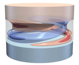
  $d$ as shown in figure 1. Short liquid bridges can be hydrostatically stable, even in a terrestrial gravity field, depending on the wetting conditions and the geometry. Here we consider an axisymmetric geometry with the axial acceleration of gravity
  $\boldsymbol {g}=-g\boldsymbol {e}_z$, where
  $\boldsymbol {e}_z$ is the axial unit vector, while the liquid is heated from above. We assume the liquid bridge is pinned to the sharp circular edges of the two support discs. The gas phase (air) is Newtonian as well and it is bounded radially by a cylindrical tube of radius
  $r_{o}>r_{i}$ (o: outer) and height
  $2d_{s}+d$, placed coaxially around the liquid bridge and the support discs. The shield cylinder was first used in experiments by Preisser et al. (Reference Preisser, Schwabe and Scharmann1983) and, more recently, by, e.g. Simic-Stefani et al. (Reference Simic-Stefani, Kawaji and Yoda2006) and Gaponenko et al. (Reference Gaponenko, Mialdun, Nepomnyashchy and Shevtsova2021). To a good approximation, it can be considered thermally insulating. Thus, the geometry of the problem is characterised by
 \begin{equation} \varGamma = \frac{d}{r_{i}},\quad \varGamma_{s}=\frac{d_{s}}{r_{i}},\quad \eta = \frac{r_{o}}{r_{i}}, \end{equation}
where  $\varGamma$ and
  $\varGamma _{s}$ describe the aspect ratios of the liquid bridge and the discs, respectively, and
  $\eta$ is the radius ratio of the annular space between the tube and the support discs.

Figure 1. Schematic of the axisymmetric thermocapillary liquid bridge including the coordinate system. The sketch shows the situation when the liquid bridge is exposed to a hot gas stream with mean axial velocity  $\bar {W}_{g,in}$. The gravity vector
  $\boldsymbol {g}$ is always aligned with the negative
  $z$ axis. The thermocapillary effect is illustrated schematically through velocity vectors close to the interface.
The support discs are kept at different but constant temperatures  $T_{hot} = \bar {T}+\Delta T/2$ and
  $T_{cold} = \bar {T}-\Delta T/2$, respectively, where
  $\Delta T=T_{hot}-T_{cold}>0$ is an imposed temperature difference. The mean temperature
  $\bar {T}=(T_{hot}+T_{cold})/2$ is used as the reference temperature
  $T^* = \bar {T}$. Owing to the imposed temperature difference the surface tension
  $\sigma (T)$ varies along the interface. Tangential surface tension gradients create surface stresses (Levich Reference Levich1962) that drive a flow on both sides of the interface via the thermocapillary effect, as sketched in figure 1. Taylor expansion of
  $\sigma (T)$ about
  $T^*$ yields the surface tension gradient
 \begin{align} \boldsymbol{\nabla}_\| \sigma(T)&= \frac{\partial\sigma}{\partial T} \boldsymbol{\nabla}_\| T = \frac{\partial}{\partial T}[\sigma^* -\gamma^* (T - T^*) + \dots]\boldsymbol{\nabla}_\| T \nonumber\\ &= \{-\gamma^* + O[(T-T^*)] \} \boldsymbol{\nabla}_\| T, \end{align}
where  $\boldsymbol {\nabla }_\| = \boldsymbol {t} (\boldsymbol {t}\boldsymbol {\cdot }\boldsymbol {\nabla })$ is the Nabla operator in the plane tangent to the interface,
  $\boldsymbol {t}$ an arbitrary unit tangent vector,
  $\gamma ^* = -\partial \sigma / \partial T\vert _{T = T^*}$ is the negative linear surface tension coefficient and
  $\sigma ^*=\sigma (T^*)$ is the reference (mean) surface tension. The asterisk indicates reference values of temperature-dependent thermophysical properties evaluated at
  $T^*$. The Taylor expansion in (2.2) is truncated after the linear term, since literature data on the coefficients of the higher-order terms for silicone oil in air are lacking. Within our modelling, we take into account the full temperature dependence of all other thermophysical properties and neglect the pressure dependence, assuming reference conditions far from phase-change critical points.
The flow in the liquid phase is driven by surface stresses that depend on the conditions in the gas phase. Thus, imposing a gas flow allows us to passively control the flow in the liquid phase by varying the temperature and velocity (magnitude, profile) of the forced gas flow at the inlet, which is located either at the upper or the lower end of the tube. Owing to the low viscosity of gases under standard conditions, the gas flow affects the motion in the liquid phase primarily by altering the surface temperature and, thus, the thermocapillary stresses, and to a lesser degree by mechanical stresses on the interface. In addition, buoyancy forces drive the flow due to horizontal density gradients. For very small liquid bridges, (thermocapillary) surface forces typically dominate (buoyant) volume forces. But for millimetric liquid bridges investigated under terrestrial conditions, buoyancy can significantly affect the interfacial shape and the fluid motion.
2.2. Governing equations and boundary conditions
2.2.1. Transport equations
Due to the axisymmetric geometry, we use cylindrical coordinates  $(r, \varphi, z)$ with the corresponding unit vectors
  $(\boldsymbol {e}_r, \boldsymbol {e}_\varphi, \boldsymbol {e}_z)$, and an origin centred in the middle of the liquid bridge. The velocity field is represented as
  $\boldsymbol {u}=u\boldsymbol {e}_r+v\boldsymbol {e}_\varphi +w\boldsymbol {e}_z$.
The fluid motion inside the liquid bridge is governed by the Navier–Stokes, continuity and energy equations. For a Newtonian fluid with variable properties, they read in strong conservative form
 $$\begin{gather} \frac{\partial (\rho \boldsymbol{u} )}{\partial t}+\boldsymbol{\nabla}\boldsymbol{\cdot} (\rho \boldsymbol{u}\boldsymbol{u}) ={-} \boldsymbol{\nabla} P +\rho g \boldsymbol{e}_z +\boldsymbol{\nabla}\boldsymbol{\cdot} (\mu \boldsymbol{\mathsf{S}} ), \end{gather}$$
 $$\begin{gather}\frac{\partial \rho}{\partial t}+\boldsymbol{\nabla}\boldsymbol{\cdot} (\rho \boldsymbol{u} ) = 0, \end{gather}$$
 $$\begin{gather}\frac{\partial(\rho c_p T )}{\partial t}+ \boldsymbol{\nabla}\boldsymbol{\cdot} (\rho c_p \boldsymbol{u} T) = \boldsymbol{\nabla}\boldsymbol{\cdot} (\lambda\boldsymbol{\nabla} T), \end{gather}$$
where  $t$ is time,
  $P$ is the pressure and
  $\boldsymbol{\mathsf{S}} = \boldsymbol {\nabla }\boldsymbol {u} + (\boldsymbol {\nabla } \boldsymbol {u})^\mathrm {T}-(2/3) (\boldsymbol {\nabla }\boldsymbol {\cdot }\boldsymbol {u})\boldsymbol{\mathsf{I}}$ the deformation rate tensor with the identity matrix
  $\boldsymbol{\mathsf{I}}$. In contrast to most previous numerical studies on liquid bridges, we consider the dynamic viscosity
  $\mu (T)$, the density
  $\rho (T)$, the specific heat capacity
  $c_p(T)$ and the thermal conductivity
  $\lambda (T)$ to be fully temperature dependent (FTD) and call this the FTD approach in contrast to, e.g. the OB approximation. The equations governing the gas phase are formally identical to (2.3). The material parameters relating to the gas phase
  $\rho _{g}$,
  $\mu _{g}$,
  $\lambda _{g}$ and
  $c_{p{g}}$ are indicated by the subscript ‘g’.
Using the reference material parameters of the liquid (superscript ‘*’) evaluated at the reference temperature  $T^*$, (2.3) are made dimensionless by the length, time, velocity, pressure and temperature scales
  $d$,
$d$,  $d^2\rho ^*/\mu ^*$,
  $\gamma ^*\Delta T/\mu ^*$,
  $\gamma ^*\Delta T/d$ and
  $\Delta T$, respectively. This yields
 $$\begin{gather} \frac{\partial ( \alpha_\rho \boldsymbol{u} )}{\partial t}+{\textit{Re}} \boldsymbol{\nabla}\boldsymbol{\cdot} (\alpha_\rho\boldsymbol{u}\boldsymbol{u}) ={-} \boldsymbol{\nabla} p-{\textit{Bd}}\frac{\alpha_\rho-\alpha_{\rho}^{*}}{\varepsilon} \boldsymbol{e}_z +\boldsymbol{\nabla} \boldsymbol{\cdot} (\alpha_\mu \boldsymbol{\mathsf{S}} ), \end{gather}$$
 $$\begin{gather}\frac{\partial \alpha_\rho }{\partial t}+{\textit{Re}}\boldsymbol{\nabla}\boldsymbol{\cdot}(\alpha_\rho \boldsymbol{u} ) = 0, \end{gather}$$
 $$\begin{gather}\frac{\partial(\alpha_\rho \alpha_{cp} \vartheta )}{\partial t}+ {\textit{Re}} \boldsymbol{\nabla}\boldsymbol{\cdot} (\alpha_\rho\alpha_{cp} \boldsymbol{u}\vartheta) =\frac{1}{{\textit{Pr}}} \boldsymbol{\nabla}\boldsymbol{\cdot} (\alpha_\lambda\boldsymbol{\nabla}\vartheta), \end{gather}$$
where  $p = (d/\gamma ^*\Delta T )(P - \rho ^* g z)$ is the reduced pressure and
 \begin{equation} \vartheta = \frac{T-T^*}{\Delta T} \end{equation}
the reduced temperature. The Reynolds, Prandtl and dynamic Bond numbers are respectively defined as
 \begin{equation} {\textit{Re}} = \frac{\rho^*\gamma^*\Delta T d}{ {\mu^*}^2}, \quad {\textit{Pr}} = \frac{\mu^* c^*_p}{\lambda^*},\quad {\textit{Bd}} = \frac{\rho^* g\beta^* d^2}{\gamma^*}. \end{equation}
 Equations (2.4) hold for both the liquid and the gas phase. They are distinguished by the functions  $\alpha (\vartheta )$ and the parameter
  $\varepsilon$. The parameters
  $\varepsilon =\beta ^*\Delta T$ and
  $\varepsilon _{g}=\beta _{g}^*\Delta T$ measure the magnitude of the density variation in the respective phase, where
  $\beta ^*=-(1/\rho ^*)(\partial \rho /\partial T)^*_P$ and
  $\beta ^*_{g}$ are the thermal expansion coefficients of the liquid and gas, respectively, evaluated at
  $\vartheta ^*=0$. As in Stojanović et al. (Reference Stojanović, Romanò and Kuhlmann2022), the phase is distinguished by selecting the respective set of thermophysical shape functions
 \begin{align} \boldsymbol{\alpha} &= \left[ \alpha_\rho(\vartheta),\alpha_\mu(\vartheta),\alpha_\lambda(\vartheta),\alpha_{cp}(\vartheta) \right] \nonumber\\ &= \begin{cases} \left[\dfrac{\rho(\vartheta)}{\rho^*},\dfrac{\mu(\vartheta)}{\mu^*},\dfrac{\lambda(\vartheta)}{\lambda^*}, \dfrac{c_p(\vartheta)}{c^*_p}\right] & \text{for the liquid phase,}\\[12pt] \left[\dfrac{\rho_{g}(\vartheta)}{\rho^*},\dfrac{\mu_{g}(\vartheta)}{\mu^*},\dfrac{\lambda_{g}(\vartheta)} {\lambda^*},\dfrac{c_{pg}(\vartheta)}{c^*_p}\right] & \text{for the gas phase,} \end{cases} \end{align}
which represent the temperature-dependent material parameters, normalised by the values that the parameters take in the liquid at the reference temperature. A shape function evaluated at the reference point is indicated by an asterisk, i.e.  $\alpha _\rho ^* = \alpha _\rho (\vartheta ^*) = 1$ for the liquid and
  $\alpha _\rho ^* = \rho _{g}^*/\rho ^*$ for the gas. The shape functions
  $\alpha _j$ with
  $j \in [\rho, \mu, \lambda, c_p]$ used will be specified in § 4. Note that in (2.4a)
  $(\alpha _\rho -\alpha _{\rho }^{*})/\varepsilon = -\vartheta + {O}(\vartheta ^2)$, recovering the buoyancy term in Boussinesq approximation at linear order. In a model assuming constant material parameters,
 \begin{equation} \boldsymbol{\alpha} = \begin{cases} [1,1,1,1] & \text{for the liquid phase,}\\ \left[\dfrac{\rho^*_{g}}{\rho^*},\dfrac{\mu^*_{g}}{\mu^*},\dfrac{\lambda^*_{g}}{\lambda^*}, \dfrac{c^*_{pg}}{c^*_p}\right] & \text{for the gas phase,} \end{cases} \end{equation}
and the bulk equations only depend on  ${\textit {Re}}$,
  ${\textit {Pr}}$ and
  ${\textit {Bd}}$.
2.2.2. Linear stability equations
For sufficiently small driving forces, measured either by the Reynolds number  ${\textit {Re}}$ or the Marangoni number
  ${\textit {Ma}}={\textit {Re}}{\textit {Pr}}$, an axisymmetric and time-independent solution
  $\boldsymbol {q}_0(r,z) = (u_0,0,w_0,p_0,\vartheta _0)$ (liquid) and
  $\boldsymbol {q}_{g0}(r,z) = (u_{g0},0,w_{g0},p_{g0},\vartheta _{g0})$ (gas) of (2.4) exists. This basic flow is indicated by a subscript ‘0’. The shape of the interface
  $h_0(z)$, separating the gas from the liquid phase, is part of the basic flow solution.
To investigate the linear stability of the basic flow, the dynamics of small deviations from the basic solution must be considered. These deviations also concern the interfacial shape. Recent experiments (Yano et al. Reference Yano, Nishino, Matsumoto, Ueno, Komiya, Kamotani and Imaishi2018b) revealed that the dynamic interfacial deformation caused by the perturbation flow is negligible. Therefore, we only consider perturbations of  $\boldsymbol {q}_0$ and
  $\boldsymbol {q}_{g0}$ within their domains separated by the phase boundary
  $h_0(z)$. To carry out the linear stability analysis, the general three-dimensional and time-dependent solution
  $[\boldsymbol {q},\boldsymbol {q}_{g}]$ of (2.4) is decomposed into
 \begin{equation} \boldsymbol{q}=\boldsymbol{q}_0(r,z)+\tilde{\boldsymbol{q}}(r,\varphi,z,t)\quad\text{and} \quad \boldsymbol{q}_{g}=\boldsymbol{q}_{{g}0}(r,z)+\tilde{\boldsymbol{q}}_{g}(r,\varphi,z,t). \end{equation}
separating the perturbation flow  $[\tilde {\boldsymbol {q}},\tilde {\boldsymbol {q}}_{g}]$ (indicated by a tilde) from the basic flow
  $[\boldsymbol {q}_0,\boldsymbol {q}_{g0}]$.
The linear dynamics is obtained by inserting (2.9a,b) in (2.4) and linearising all terms with respect to all perturbation quantities, in particular, with respect to  $\tilde {\vartheta }$. This requires linearising the shape functions
  $\alpha _j(\vartheta )$ about their local values
  $\alpha _j[\vartheta _0(r,z)]$ determined by the basic flow. Taylor expansion about the local basic state temperature
  $\vartheta _0(r,z)$ yields
 \begin{equation} \alpha_j(\vartheta) = \alpha_j(\vartheta_0 + \tilde{\vartheta}) = \alpha_j(\vartheta_0)+\left. \frac{\partial\alpha_j}{\partial \vartheta}\right|_{\vartheta_0}\tilde{\vartheta} +\, O(\tilde{\vartheta}^2) = \alpha_{j 0}+\alpha_{j 0}'\tilde{\vartheta} + O(\tilde{\vartheta}^2) , \end{equation}
where the zeroth- and first-order Taylor coefficients  $\alpha _{j 0}[\vartheta _0(r,z)]$ and
  $\alpha _{j 0}'[\vartheta _0(r,z)]$ are scalar fields that depend continuously on
  $(r,z)$ through the basic temperature field
  $\vartheta _0(r,z)$. Using (2.10) we obtain the linearised version of (2.4) as
 \begin{gather}
\alpha_{\rho 0}\frac{\partial \tilde{\boldsymbol{u}}}{\partial
t}+\alpha_{\rho 0}'\boldsymbol{u}_0\frac{\partial
\tilde{\vartheta}}{\partial t}+{\textit{Re}}
\boldsymbol{\nabla} \boldsymbol{\cdot} \left( \alpha_{\rho
0}\boldsymbol{u}_0\tilde{\boldsymbol{u}} + \alpha_{\rho
0}\tilde{\boldsymbol{u}}\boldsymbol{u}_0 + \alpha_{\rho
0}'\boldsymbol{u}_0\boldsymbol{u}_0\tilde{\vartheta}
\right)\nonumber\\ ={-} \boldsymbol{\nabla}
\tilde{p}-\frac{{\textit{Bd}}}{\varepsilon}
\alpha_{\rho 0}'\tilde{\vartheta} \boldsymbol{e}_z
+\boldsymbol{\nabla}\boldsymbol{\cdot} (\alpha_{\mu 0}
\tilde{\boldsymbol{\mathsf{S}}} +\alpha_{\mu 0}'
\boldsymbol{\mathsf{S}}_0\tilde{\vartheta} ),
\end{gather}
\begin{gather}
\alpha_{\rho 0}\frac{\partial \tilde{\boldsymbol{u}}}{\partial
t}+\alpha_{\rho 0}'\boldsymbol{u}_0\frac{\partial
\tilde{\vartheta}}{\partial t}+{\textit{Re}}
\boldsymbol{\nabla} \boldsymbol{\cdot} \left( \alpha_{\rho
0}\boldsymbol{u}_0\tilde{\boldsymbol{u}} + \alpha_{\rho
0}\tilde{\boldsymbol{u}}\boldsymbol{u}_0 + \alpha_{\rho
0}'\boldsymbol{u}_0\boldsymbol{u}_0\tilde{\vartheta}
\right)\nonumber\\ ={-} \boldsymbol{\nabla}
\tilde{p}-\frac{{\textit{Bd}}}{\varepsilon}
\alpha_{\rho 0}'\tilde{\vartheta} \boldsymbol{e}_z
+\boldsymbol{\nabla}\boldsymbol{\cdot} (\alpha_{\mu 0}
\tilde{\boldsymbol{\mathsf{S}}} +\alpha_{\mu 0}'
\boldsymbol{\mathsf{S}}_0\tilde{\vartheta} ),
\end{gather}
 \begin{gather} \alpha_{\rho
0}'\frac{\partial \tilde{\vartheta}}{\partial
t}+{\textit{Re}}\boldsymbol{\nabla}\boldsymbol{\cdot}(\alpha_{\rho
0} \tilde{\boldsymbol{u}}+\alpha_{\rho 0}' \boldsymbol{u}_0
\tilde{\vartheta}) = 0,
\end{gather}
\begin{gather} \alpha_{\rho
0}'\frac{\partial \tilde{\vartheta}}{\partial
t}+{\textit{Re}}\boldsymbol{\nabla}\boldsymbol{\cdot}(\alpha_{\rho
0} \tilde{\boldsymbol{u}}+\alpha_{\rho 0}' \boldsymbol{u}_0
\tilde{\vartheta}) = 0,
\end{gather}
 \begin{gather} {[}\alpha_{\rho 0}
\alpha_{cp 0}+\vartheta_0 (\alpha_{\rho 0}' \alpha_{cp
0}+\alpha_{\rho 0} \alpha_{cp 0}')]\frac{\partial
\tilde{\vartheta}}{\partial
t}+{\textit{Re}}\boldsymbol{\nabla}\boldsymbol{\cdot}(
\alpha_{\rho 0} \alpha_{cp 0}
\boldsymbol{u}_0\tilde{\vartheta}+\alpha_{\rho 0}
\alpha_{cp
0}\vartheta_0\tilde{\boldsymbol{u}}\nonumber\\
+\alpha_{\rho 0}' \alpha_{cp 0}
\vartheta_0\boldsymbol{u}_0
\tilde{\vartheta}+
\alpha_{\rho 0} \alpha_{cp 0}'
\vartheta_0\boldsymbol{u}_0\tilde{\vartheta})=
\frac{1}{{\textit{Pr}}}\boldsymbol{\nabla}\boldsymbol{\cdot}(\alpha_{\lambda
0}' \tilde{\vartheta} \boldsymbol{\nabla} \vartheta_0+
\alpha_{\lambda 0} \boldsymbol{\nabla}\tilde{\vartheta}),
\end{gather}
\begin{gather} {[}\alpha_{\rho 0}
\alpha_{cp 0}+\vartheta_0 (\alpha_{\rho 0}' \alpha_{cp
0}+\alpha_{\rho 0} \alpha_{cp 0}')]\frac{\partial
\tilde{\vartheta}}{\partial
t}+{\textit{Re}}\boldsymbol{\nabla}\boldsymbol{\cdot}(
\alpha_{\rho 0} \alpha_{cp 0}
\boldsymbol{u}_0\tilde{\vartheta}+\alpha_{\rho 0}
\alpha_{cp
0}\vartheta_0\tilde{\boldsymbol{u}}\nonumber\\
+\alpha_{\rho 0}' \alpha_{cp 0}
\vartheta_0\boldsymbol{u}_0
\tilde{\vartheta}+
\alpha_{\rho 0} \alpha_{cp 0}'
\vartheta_0\boldsymbol{u}_0\tilde{\vartheta})=
\frac{1}{{\textit{Pr}}}\boldsymbol{\nabla}\boldsymbol{\cdot}(\alpha_{\lambda
0}' \tilde{\vartheta} \boldsymbol{\nabla} \vartheta_0+
\alpha_{\lambda 0} \boldsymbol{\nabla}\tilde{\vartheta}),
\end{gather}
where  $\tilde {\boldsymbol{\mathsf{S}}} = \boldsymbol {\nabla }\tilde {\boldsymbol {u}} + (\boldsymbol {\nabla } \tilde {\boldsymbol {u}})^\mathrm {T} -(2/3)(\boldsymbol {\nabla }\boldsymbol {\cdot }\tilde {\boldsymbol {u}})\boldsymbol{\mathsf{I}}$ and
  $\boldsymbol{\mathsf{S}}_0 = \boldsymbol {\nabla }\boldsymbol {u}_0 + (\boldsymbol {\nabla }\boldsymbol {u}_0)^\mathrm {T} - (2/3)(\boldsymbol {\nabla }\boldsymbol {\cdot }\boldsymbol {u}_0 )\boldsymbol{\mathsf{I}}$. The basic state solution enters parametrically in the linear disturbance equations for
  $\tilde {\boldsymbol {q}}$.
Since (2.11) is linear in  $\tilde {\boldsymbol {q}}$ with coefficients that do not depend on
  $\varphi$ and
  $t$, the general solution
  $\tilde {\boldsymbol {q}}$ of (2.11) can be constructed by a superposition of normal modes
 \begin{align} \tilde{\boldsymbol{q}}=\sum_{j,m} \hat{\boldsymbol{q}}_{j,m}(r,z)\exp (\psi_{j,m}t+\mathrm{i} m\varphi)+\text{c.c.},\quad \tilde{\boldsymbol{q}}_{g}=\sum_{j,m} \hat{\boldsymbol{q}}_{{g}j,m}(r,z)\exp (\psi_{j,m}t+\mathrm{i} m\varphi)+\text{c.c.}, \end{align}
where the complex conjugates terms (c.c.) render the solution real. The normal modes are harmonic in  $\varphi$ with wavenumber
  $m \in \mathbb {N}_0$. The time dependence of each mode is exponential with the complex growth
  $\psi _{j,m} \in \mathbb {C}$. The index
  $j$ numbers the discrete set of solutions for fixed
  $m$ that arise due to the finite domain in
  $r$ and
  $z$. Inserting the ansatz (2.12a,b) into (2.11) yields partial differential equations for the complex amplitudes
  $\hat {\boldsymbol {q}}_{j,m}$ and
  $\hat {\boldsymbol {q}}_{{g}j,m}$,
 \begin{align}
&\psi\left(\boldsymbol{u}_0\alpha_{\rho 0}' \hat{\vartheta}
+\alpha_{\rho 0} \hat{\boldsymbol{u}}\right)+
{\textit{Re}}\boldsymbol{\nabla}\boldsymbol{\cdot}\left[\alpha_{\rho
0}'
\hat{\vartheta}\boldsymbol{u}_0\boldsymbol{u}_0+\alpha_{\rho
0}(\boldsymbol{u}_0\hat{\boldsymbol{u}}+\hat{\boldsymbol{u}}\boldsymbol{u}_0)\right]+{\textit{Re}}\frac{\alpha_{\rho
0}\mathrm{i} \hat{v}m\boldsymbol{u}_0}{r}\nonumber\\ &\quad
={-}\boldsymbol{\nabla}
\hat{p}-\frac{{\textit{Bd}}}{\varepsilon}\alpha_{\rho
0}'\hat{\vartheta}\boldsymbol{e}_z+\boldsymbol{\nabla}\boldsymbol{\cdot}\left(\alpha_{\mu
0}' \hat{\vartheta} \boldsymbol{\mathsf{S}}_0+\alpha_{\mu 0}
\hat{\boldsymbol{\mathsf{S}}}\right)+\left(\alpha_{\mu 0}'
\hat{\vartheta} \boldsymbol{\mathsf{S}}_0+\alpha_{\mu 0}
\hat{\boldsymbol{\mathsf{S}}}-\hat{p} \right)\frac{\mathrm{i} m
\boldsymbol{e}_\varphi}{r}
\end{align}
\begin{align}
&\psi\left(\boldsymbol{u}_0\alpha_{\rho 0}' \hat{\vartheta}
+\alpha_{\rho 0} \hat{\boldsymbol{u}}\right)+
{\textit{Re}}\boldsymbol{\nabla}\boldsymbol{\cdot}\left[\alpha_{\rho
0}'
\hat{\vartheta}\boldsymbol{u}_0\boldsymbol{u}_0+\alpha_{\rho
0}(\boldsymbol{u}_0\hat{\boldsymbol{u}}+\hat{\boldsymbol{u}}\boldsymbol{u}_0)\right]+{\textit{Re}}\frac{\alpha_{\rho
0}\mathrm{i} \hat{v}m\boldsymbol{u}_0}{r}\nonumber\\ &\quad
={-}\boldsymbol{\nabla}
\hat{p}-\frac{{\textit{Bd}}}{\varepsilon}\alpha_{\rho
0}'\hat{\vartheta}\boldsymbol{e}_z+\boldsymbol{\nabla}\boldsymbol{\cdot}\left(\alpha_{\mu
0}' \hat{\vartheta} \boldsymbol{\mathsf{S}}_0+\alpha_{\mu 0}
\hat{\boldsymbol{\mathsf{S}}}\right)+\left(\alpha_{\mu 0}'
\hat{\vartheta} \boldsymbol{\mathsf{S}}_0+\alpha_{\mu 0}
\hat{\boldsymbol{\mathsf{S}}}-\hat{p} \right)\frac{\mathrm{i} m
\boldsymbol{e}_\varphi}{r}
\end{align} \begin{equation} \psi\alpha_{\rho 0}'\hat{\vartheta}+{\textit{Re}}\boldsymbol{\nabla}\boldsymbol{\cdot}\left(\alpha_{\rho 0}\hat{\boldsymbol{u}}+\alpha_{\rho 0}'\boldsymbol{u}_0\hat{\vartheta}\right)+{\textit{Re}}\frac{\alpha_{\rho 0}\mathrm{i}\hat{v}m}{r}=0, \end{equation}
 \begin{align} &\psi\left[\vartheta_0 (\alpha_{\rho 0}' \alpha_{cp0}+\alpha_{\rho 0} \alpha_{cp0}')+\alpha_{\rho 0} \alpha_{cp0}\right] \hat{\vartheta}\nonumber\\ &\quad +{\textit{Re}}\boldsymbol{\nabla}\boldsymbol{\cdot} \left[(\alpha_{\rho 0}' \alpha_{cp0}+\alpha_{\rho 0} \alpha_{cp0}') \vartheta_0\boldsymbol{u}_0 \hat{\vartheta}+\alpha_{\rho 0} \alpha_{cp0} \hat{\vartheta}\boldsymbol{u}_0+\alpha_{\rho 0} \alpha_{cp0} \vartheta_0\hat{\boldsymbol{u}}\right]\nonumber\\ &\quad +{\textit{Re}}\frac{\alpha_{\rho 0} \alpha_{cp0}\mathrm{i} \hat{v} m}{r}=\frac{1}{{\textit{Pr}}}\boldsymbol{\nabla}\boldsymbol{\cdot}\left[ (\alpha_{\lambda 0}' \hat{\vartheta} \boldsymbol{\nabla} \vartheta_0+\alpha_{\lambda 0} \boldsymbol{\nabla} \hat{\vartheta})-\frac{\alpha_{\lambda 0} \hat{\vartheta} m^2}{r^2}\right]. \end{align}
Discretisation of (2.13) leads to a large linear eigenvalue problem that must be solved to determine the stability boundary (§ 3).
2.2.3. Boundary conditions
The equations for the steady two-dimensional basic flow  $\boldsymbol {q}_0$ satisfying (2.4) and those for the perturbation amplitudes
  $\hat {\boldsymbol {q}}$ according to the linear stability equations (2.11) must be solved subject to boundary and coupling conditions.
Solid walls: On all solid walls, the liquid and gas must satisfy the no-slip conditions
 \begin{equation} \boldsymbol{u}_0=\boldsymbol{u}_{g0} = 0 \quad\text{and}\quad \hat{\boldsymbol{u}}=\hat{\boldsymbol{u}}_{g} = 0. \end{equation}
In contrast to the outer shield, which is thermally insulated in the radial direction, the cylindrical support discs are assumed to be perfect heat conductors, leading to
 \begin{equation} \text{hot disc: } \quad \vartheta_0=\vartheta_\text{g0}= 1/2 \quad \text{and} \quad \hat{\vartheta}=\hat{\vartheta}_\text{g} = 0, \end{equation}
 \begin{equation} \text{cold disc: } \quad \vartheta_0=\vartheta_\text{g0}= -1/2 \quad \text{and} \quad \hat{\vartheta}=\hat{\vartheta}_\text{g} = 0, \end{equation}
 \begin{equation} \text{shield tube: } \quad \partial \vartheta_\text{g0} / \partial r =0 \quad \text{and} \quad \partial \hat{\vartheta}_\text{g}/\partial r =0. \end{equation}
The amplitudes of the temperature perturbations vanish on the hot and cold walls since the imposed constant temperatures are taken care of by the basic state.
Axis of symmetry: On the axis  $r=0$ the symmetry of the basic state requires
 \begin{equation} u_0=\frac{\partial w_0}{\partial r}=\frac{\partial \vartheta_0}{\partial r}=0. \end{equation}
The boundary conditions for the perturbation amplitudes depend on the azimuthal wavenumber  $m$ and are given in table 1.
Table 1. Boundary conditions for the perturbation flow on  $r=0$.

Liquid–gas interface: The liquid and gas flow are coupled via the interface at  $r = h_0(z)$ that is assumed to be determined by the basic flow only. Therefore, we first consider the basic flow. The continuity of the basic temperature and the basic heat flux requires
 $$\begin{gather} r=h_0\text{: } \quad \vartheta_0 = \vartheta_{g0}, \end{gather}$$
 $$\begin{gather}r=h_0\text{: } \quad \alpha_{\lambda 0} \boldsymbol{n}\boldsymbol{\cdot}\boldsymbol{\nabla}\vartheta_0 = \alpha_{\lambda {g0}} \boldsymbol{n}\boldsymbol{\cdot}\boldsymbol{\nabla}\vartheta_\text{g0}, \end{gather}$$
where
 \begin{equation} \boldsymbol{n} = \frac{1}{N}\left(\boldsymbol{e}_r -\frac{\mathrm{d} h_0}{\mathrm{d} z}\boldsymbol{e}_z \right) \quad \text{with} \ N=\sqrt{1+\left(\frac{\mathrm{d} h_0}{\mathrm{d} z}\right)^2}, \end{equation}
is the outward-pointing unit normal vector to the interface. The kinematic coupling conditions
 \begin{equation} r=h_0\text{: } \quad \boldsymbol{u}_0 = \boldsymbol{u}_{g0} \quad \text{and} \quad \frac{u_0}{w_0}=\frac{\mathrm{d} h_0}{\mathrm{d} z} \end{equation}
guarantee no slip on the interface and also enforce the basic streamlines to be parallel to the interface  $h_0(z)$.
The dynamic coupling condition is represented by the stress balance on the interface. It is decomposed into a normal stress balance
 \begin{align} &-(p_0-p_{g0}) +
\alpha_{\mu 0}\boldsymbol{n} \boldsymbol{\cdot}
\boldsymbol{\mathsf{S}}_0 \boldsymbol{\cdot} \boldsymbol{n} + \left(
\frac{1}{{\textit{Ca}}} -\vartheta_0\right)
\boldsymbol{\nabla}\boldsymbol{\cdot}\boldsymbol{n}
\nonumber\\ &\quad ={-}(\alpha_{\rho 0}-\alpha_{\rho
{g}0})\frac{{\textit{Bo}}}{{\textit{Ca}}}z+\alpha_{\mu
{g}0}\boldsymbol{n} \boldsymbol{\cdot} \boldsymbol{\mathsf{S}}_{g0}
\boldsymbol{\cdot} \boldsymbol{n},
\end{align}
\begin{align} &-(p_0-p_{g0}) +
\alpha_{\mu 0}\boldsymbol{n} \boldsymbol{\cdot}
\boldsymbol{\mathsf{S}}_0 \boldsymbol{\cdot} \boldsymbol{n} + \left(
\frac{1}{{\textit{Ca}}} -\vartheta_0\right)
\boldsymbol{\nabla}\boldsymbol{\cdot}\boldsymbol{n}
\nonumber\\ &\quad ={-}(\alpha_{\rho 0}-\alpha_{\rho
{g}0})\frac{{\textit{Bo}}}{{\textit{Ca}}}z+\alpha_{\mu
{g}0}\boldsymbol{n} \boldsymbol{\cdot} \boldsymbol{\mathsf{S}}_{g0}
\boldsymbol{\cdot} \boldsymbol{n},
\end{align}and a tangential stress balance
 \begin{equation} \alpha_{\mu
0}\boldsymbol{t}\boldsymbol{\cdot}\boldsymbol{\mathsf{S}}_0\boldsymbol{\cdot}\boldsymbol{n}
={-}\boldsymbol{t}\boldsymbol{\cdot} \boldsymbol{\nabla}
\vartheta_0 +\alpha_{\mu
{g}0}\boldsymbol{t}\boldsymbol{\cdot}\boldsymbol{\mathsf{S}}_{g0}\boldsymbol{\cdot}\boldsymbol{n},
\end{equation}
\begin{equation} \alpha_{\mu
0}\boldsymbol{t}\boldsymbol{\cdot}\boldsymbol{\mathsf{S}}_0\boldsymbol{\cdot}\boldsymbol{n}
={-}\boldsymbol{t}\boldsymbol{\cdot} \boldsymbol{\nabla}
\vartheta_0 +\alpha_{\mu
{g}0}\boldsymbol{t}\boldsymbol{\cdot}\boldsymbol{\mathsf{S}}_{g0}\boldsymbol{\cdot}\boldsymbol{n},
\end{equation}
where  $\boldsymbol {t}\perp \boldsymbol {n}$ is the unit tangent vector, and the basic state shape functions, like
  $\alpha _{\mu {g}0}(r,z)$, depend on
  $(r,z)$. In these non-dimensional equations
 \begin{equation} {\textit{Ca}}=\frac{\gamma^*\Delta T}{\sigma^*} \quad\text{and}\quad {\textit{Bo}} =\frac{\rho^*g d^2}{\sigma^*} \end{equation}
denote the capillary number and the static Bond number, respectively. Since the term  $(\alpha _{\rho 0}-\alpha _{\rho {g}0})$ in (2.20a) takes care of the static pressure distribution in the gas phase, the reference density of the gas
  $\rho _{g}^*$ does not enter
  ${\textit {Bo}}$. This way, the non-dimensional material parameter
 \begin{equation} \tau=\frac{\rho^*\beta^*\sigma^*}{\gamma^*} = \frac{{\textit{Bd}}}{{\textit{Bo}}}=\frac{\varepsilon}{{\textit{Ca}}} \end{equation}
serves as a proportionality factor between the dynamic and static Bond numbers and also between  $\varepsilon$ and
  ${\textit {Ca}}$.
Since the location  $h_0(z)$ is part of the basic flow solution, it is obtained iteratively by solving simultaneously the Navier–Stokes equations for both phases and imposing the coupling and boundary conditions. To that end, we assume the contact lines are pinned to the edges of the support discs,
  $h_0(\pm 1/2)=1/\varGamma$, and impose the volume constraint
 \begin{equation} \varGamma^2\int_{{-}1/2}^{1/2} h_0(z)^2\,\mathrm{d} z=\mathcal{V}, \end{equation}
where  $\mathcal {V}=V/{\rm \pi} r_{i}^2d$ is the ratio between the volume
  $V$ occupied by the liquid and the upright cylindrical volume between the two support discs.
To assess the influence of the dynamic deformability of a dynamic interface (DI), we also consider a static interface (SI) whose shape  $h_0(z)$, instead by the normal stress balance (2.20a), is determined by the solution of the Young–Laplace equation
 \begin{equation} \Delta p_h =\frac{\boldsymbol{\nabla}\boldsymbol{\cdot}\boldsymbol{n}}{{\textit{Ca}}} + \frac{{\textit{Bo}}}{{\textit{Ca}}} z, \end{equation}
where  $\Delta p_h$ is a constant pressure jump across the interface. For more details, see Stojanović et al. (Reference Stojanović, Romanò and Kuhlmann2022).
Once the interface shape  $h_0(z)$ and the basic state are computed, the coupling conditions for the perturbation amplitudes
 \begin{equation} \hat{\vartheta} = \hat{\vartheta}_{g},\quad \alpha_{\lambda 0} \boldsymbol{n}\boldsymbol{\cdot} \boldsymbol{\nabla}\hat{\vartheta} = \alpha_{\lambda {g}0} \boldsymbol{n}\boldsymbol{\cdot} \boldsymbol{\nabla}\hat{\vartheta}_{g},\quad \hat{\boldsymbol{u}} = \hat{\boldsymbol{u}}_{g} \end{equation}
and
 \begin{equation} \alpha_{\mu 0}\boldsymbol{t}\boldsymbol{\cdot}\hat{\boldsymbol{\mathsf{S}}}\boldsymbol{\cdot}\boldsymbol{n} ={-}\boldsymbol{t} \boldsymbol{\cdot}\boldsymbol{\nabla} \hat{\vartheta} +\alpha_{\mu {g}0}\boldsymbol{t}\boldsymbol{\cdot}\hat{\boldsymbol{\mathsf{S}}}_{g}\boldsymbol{\cdot}\boldsymbol{n} \end{equation}
can readily be imposed to solve the perturbation equations (2.13).
Inlet and outlet conditions: The boundary conditions at the ends of the shield tube,  $z=\pm (1/2+\varGamma _{s}/\varGamma )$, depend on whether the tube is sealed or open. In the case of a sealed tube, we prescribe no-slip and adiabatic conditions on both plane end walls, i.e.
 \begin{equation} \boldsymbol{u}_{g0} = \hat{\boldsymbol{u}}_{g} = 0 \quad\text{and}\quad \partial\vartheta_{g0}/\partial z=\partial\hat{\vartheta}_{g}/\partial z=0. \end{equation}
For an open tube, upflow in the positive  $z$ direction and downflow in the negative
  $z$ direction are distinguished by the sign of the Reynolds number
  ${Re}_{g} = \bar {W}_{g,in}\rho ^*d/\mu ^*$, defined as in Stojanovic, Romanò & Kuhlmann (Reference Stojanović, Romanò and Kuhlmann2023), which is taken positive for upflow and negative for downflow. The inlet
  $(z_{in})$ and outlet locations
  $(z_{out})$ are thus defined as
 \begin{equation} z_{in}={\pm}\left(1/2+\varGamma_{s}/\varGamma\right) ={-}z_{out} \quad \text{for}\ {Re}_{g} \lessgtr 0. \end{equation}
At the inlet, we prescribe a fully developed axial velocity profile
 \begin{equation} w_{g,in}(r) =\frac{{Re}_{g}}{{\textit{Re}}}\frac{2 \ln (\eta)}{\left(\eta^2+1 \right) \ln (\eta) -\eta^2+1}\left[1-\varGamma^2 r^2+ \left( \eta^2-1 \right)\frac{\ln (\varGamma r)}{\ln (\eta)} \right], \end{equation}
where the factor  ${\textit {Re}}^{-1}$ arises due to the scaling. The unconventional gas Reynolds number
  ${Re}_{g}$ is defined combining the mean inlet velocity of the gas and the kinematic viscosity of the liquid
  $\mu ^*/\rho ^*$. The usefulness of
  ${Re}_{g}$ defined in this way is explained in Appendix A of Stojanovic et al. (Reference Stojanović, Romanò and Kuhlmann2023): it provides a better correlation of the critical Reynolds numbers, because the instability arises in the liquid and not in the gas.
At the outlet, outflow conditions are used such that
 $$\begin{gather} z=z_{in}\text{: }\quad w_{g0}=w_{g,in}(r) \quad \text{and}\quad u_{g0}= \hat{u}_{g}=\hat{v}_{g}=\hat{w}_{g}=0, \end{gather}$$
 $$\begin{gather}z=z_{out}\text{: }\quad \partial u_{g0}/\partial z=\partial w_{g0}/\partial z=0 \quad \text{and}\quad \partial\hat{u}_{g}/\partial z=\partial\hat{v}_{g}/\partial z= \partial\hat{w}_{g}/\partial z=0. \end{gather}$$
Following Stojanović, Romanò & Kuhlmann (Reference Stojanović, Romanò and Kuhlmann2023a), constant temperatures are imposed at both ends of the tube
 \begin{equation} z={\pm} \left(1/2+\varGamma_{s}/\varGamma\right) \text{: }\quad \vartheta_{g0}={\pm} 1/2 \quad\text{and}\quad \hat{\vartheta}_{g}=0, \end{equation}
which are equal to the temperature of the respective adjacent support disc.
3. Numerical methods
All numerical calculations required to compute the basic flow and its linear stability are carried out using the code MaranStable (Stojanović, Romanò & Kuhlmann Reference Stojanović, Romanò and Kuhlmann2023b). It is written in Matlab and is available as open source from https://github.com/fromano88/MaranStable. The stability analysis implemented in MaranStable has been verified and validated extensively for statically and dynamically deformed liquid bridges, for single- and two-phase flows where the gas phase is confined to a cylindrical tube about the liquid bridge being either closed or subject to through flow (Stojanović et al. Reference Stojanović, Romanò and Kuhlmann2022; Stojanovic et al. Reference Stojanović, Romanò and Kuhlmann2023). Grid convergence of MaranStable has been proven for a Boussinesq fluid of  ${\textit {Pr}}=28$ (Stojanović et al. Reference Stojanović, Romanò and Kuhlmann2022). Additional verifications and validations of MaranStable regarding the FTD properties are provided in Appendix B.
3.1. Basic flow
In MaranStable the governing equations (2.4) and the boundary and coupling conditions are discretised by finite volumes using body-fitted coordinates. The physical mesh fitted to the interface shape is mapped to an orthogonal computational mesh using the surface shape  $h_0(z)$. It is computed together with the flow field updating the physical and computational meshes after every iteration step. The resulting set of nonlinear algebraic equations is linearised and solved iteratively using the Newton–Raphson method. At the
  $k$th iteration the known approximation
  $\boldsymbol {q}_0^{(k)}$ is updated by the increment
  $\delta \boldsymbol {q}$ to obtain the improved approximation
 \begin{equation} \boldsymbol{q}_0^{(k+1)} = \boldsymbol{q}_0^{(k)} + \delta \boldsymbol{q}. \end{equation}
Within the present FTD parameter approach, the nonlinear shape functions as well need to be linearised about their basic state value according to
 \begin{equation} \alpha_j\left(\vartheta_0^{(k+1)}\right)=\alpha_j\left(\vartheta_0^{(k)}+\delta \vartheta\right)\approx\alpha_j\left(\vartheta_0^{(k)}\right)+\left. \frac{\partial\alpha_j}{\partial\vartheta}\right|_{\vartheta_0^{(k)}}\delta\vartheta:= \alpha_{j0}^{(k)}+\alpha_{j0}'^{(k)}\delta\vartheta, \end{equation}
where the increment  $\delta \vartheta$ is contained in
  $\delta \boldsymbol {q}$. Inserting (3.1) and (3.2) into (2.4) yields the set of linear equations
 \begin{equation} \boldsymbol{J}\left(\boldsymbol{q}_0^{(k)}\right)\boldsymbol{\cdot} \delta \boldsymbol{q} ={-}\boldsymbol{f}\left(\boldsymbol{q}_0^{(k)}\right), \end{equation}
where  $\boldsymbol {J}(\boldsymbol {q}_0^{(k)})$ and
  $\boldsymbol {f}(\boldsymbol {q}_0^{(k)})$ are the Jacobian operator and the nonlinear residual of the Navier–Stokes equations, respectively. This leads to the linearised momentum, continuity and energy equations
 \begin{align} &{\textit{Re}}\boldsymbol{\nabla}\boldsymbol{\cdot}\left[\alpha_{\rho 0}^{(k)} \left(\boldsymbol{u}_0^{(k)}\delta\boldsymbol{u}+\delta\boldsymbol{u}\boldsymbol{u}_0^{(k)}\right) +\alpha_{\rho 0}'^{(k)}\boldsymbol{u}_0^{(k)}\boldsymbol{u}_0^{(k)}\delta\vartheta \right]\nonumber\\ &\qquad +\boldsymbol{\nabla} \delta p+\frac{{\textit{Bd}}}{\varepsilon} \alpha_{\rho 0}'^{(k)}\delta \vartheta-\boldsymbol{\nabla}\boldsymbol{\cdot}\left(\alpha_{\mu 0}^{(k)} \delta\boldsymbol{\mathsf{S}} -\alpha_{\mu 0}'^{(k)} \boldsymbol{\mathsf{S}}_0^{(k)}\delta\vartheta \right)\nonumber\\ &\quad ={-}{\textit{Re}}\boldsymbol{\nabla}\boldsymbol{\cdot}\left(\alpha_{\rho 0}^{(k)}\boldsymbol{u}_0^{(k)}\boldsymbol{u}_0^{(k)}\right) - \boldsymbol{\nabla} p_0^{(k)}-\frac{{\textit{Bd}}}{\varepsilon}\left( \alpha_{\rho 0}^{(k)} \boldsymbol{e}_z-\alpha_{\rho}^{*}\right) +\boldsymbol{\nabla}\boldsymbol{\cdot}\left(\alpha_{\mu 0}^{(k)} \boldsymbol{\mathsf{S}}_0^{(k)} \right), \end{align}
 \begin{equation} {\boldsymbol{\nabla}\boldsymbol{\cdot}\left(\alpha_{\rho 0}^{(k)} \delta\boldsymbol{u}+\alpha_{\rho 0}'^{(k)} \boldsymbol{u}_0^{(k)} \delta\vartheta\right) ={-}\boldsymbol{\nabla}\boldsymbol{\cdot}\left(\alpha_{\rho 0}^{(k)} \boldsymbol{u}_0^{(k)}\right),} \end{equation}
 \begin{align} & {\textit{Ma}} \boldsymbol{\nabla}\boldsymbol{\cdot}\left[\alpha_{\rho 0}^{(k)} \alpha_{cp 0}^{(k)}\left( \boldsymbol{u}_0^{(k)}\delta\vartheta + \vartheta_0^{(k)}\delta\boldsymbol{u}\right) + \left(\alpha_{\rho 0}'^{(k)} \alpha_{cp 0}^{(k)} + \alpha_{\rho 0}^{(k)} \alpha_{cp 0}'^{(k)} \right)\vartheta_0^{(k)}\boldsymbol{u}_0^{(k)} \delta\vartheta\right]\nonumber\\ &\quad -\boldsymbol{\nabla}\boldsymbol{\cdot}\left(\alpha_{\lambda 0}'^{(k)} \delta\vartheta \boldsymbol{\nabla} \vartheta_0^{(k)} +\alpha_{\lambda 0}^{(k)} \boldsymbol{\nabla} \delta\vartheta\right) =\boldsymbol{\nabla}\boldsymbol{\cdot}\left(\alpha_{\lambda 0}^{(k)} \boldsymbol{\nabla} \vartheta_0^{(k)}\right)-{\textit{Ma}}\boldsymbol{\nabla}\boldsymbol{\cdot} \left(\alpha_{\rho 0}^{(k)} \alpha_{cp 0}^{(k)}\boldsymbol{u}_0^{(k)}\vartheta_0^{(k)}\right), \end{align}
where  $\delta \boldsymbol{\mathsf{S}} = \boldsymbol {\nabla } \delta \boldsymbol {u} + (\boldsymbol {\nabla } \delta \boldsymbol {u})^\mathrm {T} - (2/3) (\boldsymbol {\nabla }\boldsymbol {\cdot }\delta \boldsymbol {u}) \boldsymbol{\mathsf{I}}$. An additional iteration loop arising from the normal stress balance (2.20a) is embedded in the Newton–Raphson iteration that updates the surface shape
  $h_0(z)$ after each iteration step. Neglecting terms of order
  $O(\vartheta ^2)$ in
  $\sigma (\vartheta )$, the linearised normal stress balance becomes
 \begin{align} &-(\delta p-\delta p_{g})
+ \alpha_{\mu 0}^{(k)}\boldsymbol{n}^{(k)}
\boldsymbol{\cdot} \delta\boldsymbol{\mathsf{S}} \boldsymbol{\cdot}
\boldsymbol{n}^{(k)} + \alpha_{\mu
0}^{(k)}\boldsymbol{n}^{(k)} \boldsymbol{\cdot}
\boldsymbol{\mathsf{S}}_0^{(k)} \boldsymbol{\cdot} \delta\boldsymbol{n}
+ \alpha_{\mu 0}^{(k)}\delta\boldsymbol{n}
\boldsymbol{\cdot} \boldsymbol{\mathsf{S}}_0^{(k)} \boldsymbol{\cdot}
\boldsymbol{n}^{(k)}\nonumber\\ &\quad+ \alpha_{\mu
0}'^{(k)}\boldsymbol{n}^{(k)} \boldsymbol{\cdot}
\boldsymbol{\mathsf{S}}_0^{(k)} \boldsymbol{\cdot}
\boldsymbol{n}^{(k)}\delta\vartheta+ \left(
\frac{1}{{\textit{Ca}}} -\vartheta_0^{(k)}\right)
\boldsymbol{\nabla}\boldsymbol{\cdot}\delta\boldsymbol{n}-\boldsymbol{\nabla}\boldsymbol{\cdot}
\boldsymbol{n}^{(k)}\delta\vartheta+\left(\alpha_{\rho
0}'^{(k)}-\alpha_{\rho
{g}0}'^{(k)}\right)\frac{{\textit{Bo}}}{{\textit{Ca}}}\delta\vartheta
z\nonumber\\ &\quad -\alpha_{\mu{g}
0}^{(k)}\boldsymbol{n}^{(k)} \boldsymbol{\cdot}
\delta\boldsymbol{\mathsf{S}}_{g} \boldsymbol{\cdot}
\boldsymbol{n}^{(k)} - \alpha_{\mu{g}
0}^{(k)}\boldsymbol{n}^{(k)} \boldsymbol{\cdot}
\boldsymbol{\mathsf{S}}_{{g}0}^{(k)} \boldsymbol{\cdot}
\delta\boldsymbol{n} - \alpha_{\mu{g}
0}^{(k)}\delta\boldsymbol{n} \boldsymbol{\cdot}
\boldsymbol{\mathsf{S}}_{{g}0}^{(k)} \boldsymbol{\cdot}
\boldsymbol{n}^{(k)} \nonumber\\ &\quad- \alpha_{\mu{g}
0}'^{(k)}\boldsymbol{n}^{(k)} \boldsymbol{\cdot}
\boldsymbol{\mathsf{S}}_{{g}0}^{(k)} \boldsymbol{\cdot}
\boldsymbol{n}^{(k)}\delta\vartheta=p_0^{(k)}-
p_{g0}^{(k)}-\left(\alpha_{\rho 0}^{(k)}-\alpha_{\rho
{g}0}^{(k)}\right)\frac{{\textit{Bo}}}{{\textit{Ca}}}z-\alpha_{\mu
0}^{(k)}\boldsymbol{n}^{(k)} \boldsymbol{\cdot}
\boldsymbol{\mathsf{S}}_0^{(k)} \boldsymbol{\cdot}
\boldsymbol{n}^{(k)}\nonumber\\ &\quad-\left(
\frac{1}{{\textit{Ca}}}
-\vartheta_0^{(k)}\right)\boldsymbol{\nabla}\boldsymbol{\cdot}\boldsymbol{n}^{(k)}+\alpha_{\mu
{g}0}^{(k)}\boldsymbol{n}^{(k)} \boldsymbol{\cdot}
\boldsymbol{\mathsf{S}}_{g0}^{(k)} \boldsymbol{\cdot}
\boldsymbol{n}^{(k)},
\end{align}
\begin{align} &-(\delta p-\delta p_{g})
+ \alpha_{\mu 0}^{(k)}\boldsymbol{n}^{(k)}
\boldsymbol{\cdot} \delta\boldsymbol{\mathsf{S}} \boldsymbol{\cdot}
\boldsymbol{n}^{(k)} + \alpha_{\mu
0}^{(k)}\boldsymbol{n}^{(k)} \boldsymbol{\cdot}
\boldsymbol{\mathsf{S}}_0^{(k)} \boldsymbol{\cdot} \delta\boldsymbol{n}
+ \alpha_{\mu 0}^{(k)}\delta\boldsymbol{n}
\boldsymbol{\cdot} \boldsymbol{\mathsf{S}}_0^{(k)} \boldsymbol{\cdot}
\boldsymbol{n}^{(k)}\nonumber\\ &\quad+ \alpha_{\mu
0}'^{(k)}\boldsymbol{n}^{(k)} \boldsymbol{\cdot}
\boldsymbol{\mathsf{S}}_0^{(k)} \boldsymbol{\cdot}
\boldsymbol{n}^{(k)}\delta\vartheta+ \left(
\frac{1}{{\textit{Ca}}} -\vartheta_0^{(k)}\right)
\boldsymbol{\nabla}\boldsymbol{\cdot}\delta\boldsymbol{n}-\boldsymbol{\nabla}\boldsymbol{\cdot}
\boldsymbol{n}^{(k)}\delta\vartheta+\left(\alpha_{\rho
0}'^{(k)}-\alpha_{\rho
{g}0}'^{(k)}\right)\frac{{\textit{Bo}}}{{\textit{Ca}}}\delta\vartheta
z\nonumber\\ &\quad -\alpha_{\mu{g}
0}^{(k)}\boldsymbol{n}^{(k)} \boldsymbol{\cdot}
\delta\boldsymbol{\mathsf{S}}_{g} \boldsymbol{\cdot}
\boldsymbol{n}^{(k)} - \alpha_{\mu{g}
0}^{(k)}\boldsymbol{n}^{(k)} \boldsymbol{\cdot}
\boldsymbol{\mathsf{S}}_{{g}0}^{(k)} \boldsymbol{\cdot}
\delta\boldsymbol{n} - \alpha_{\mu{g}
0}^{(k)}\delta\boldsymbol{n} \boldsymbol{\cdot}
\boldsymbol{\mathsf{S}}_{{g}0}^{(k)} \boldsymbol{\cdot}
\boldsymbol{n}^{(k)} \nonumber\\ &\quad- \alpha_{\mu{g}
0}'^{(k)}\boldsymbol{n}^{(k)} \boldsymbol{\cdot}
\boldsymbol{\mathsf{S}}_{{g}0}^{(k)} \boldsymbol{\cdot}
\boldsymbol{n}^{(k)}\delta\vartheta=p_0^{(k)}-
p_{g0}^{(k)}-\left(\alpha_{\rho 0}^{(k)}-\alpha_{\rho
{g}0}^{(k)}\right)\frac{{\textit{Bo}}}{{\textit{Ca}}}z-\alpha_{\mu
0}^{(k)}\boldsymbol{n}^{(k)} \boldsymbol{\cdot}
\boldsymbol{\mathsf{S}}_0^{(k)} \boldsymbol{\cdot}
\boldsymbol{n}^{(k)}\nonumber\\ &\quad-\left(
\frac{1}{{\textit{Ca}}}
-\vartheta_0^{(k)}\right)\boldsymbol{\nabla}\boldsymbol{\cdot}\boldsymbol{n}^{(k)}+\alpha_{\mu
{g}0}^{(k)}\boldsymbol{n}^{(k)} \boldsymbol{\cdot}
\boldsymbol{\mathsf{S}}_{g0}^{(k)} \boldsymbol{\cdot}
\boldsymbol{n}^{(k)},
\end{align}where the surface increment
 \begin{equation} \delta h_0=h_0^{(k+1)}-h_0^{(k)} \end{equation}
is contained implicitly in the increment of the surface normal vector
 \begin{equation} \delta\boldsymbol{n}=\boldsymbol{n}^{(k+1)}-\boldsymbol{n}^{(k)} \end{equation}
with
 \begin{equation} \delta\boldsymbol{n}={-}\frac{1}{N^{(k)^3}}\frac{\mathrm{d} h_0^{(k)}}{\mathrm{d} z}\frac{\mathrm{d} \delta h_0}{\mathrm{d} z}\boldsymbol{e}_r - \frac{1}{N^{(k)}}\left[1- \frac{1}{N^{(k)^2}}\left(\frac{\mathrm{d} h_0^{(k)}}{\mathrm{d} z}\right)^2\right]\frac{\mathrm{d} \delta h_0}{\mathrm{d} z}\boldsymbol{e}_z \end{equation}
and its divergence
 \begin{align} &\boldsymbol{\nabla}\boldsymbol{\cdot}\delta \boldsymbol{n} \nonumber\\ &\quad = \frac{1}{h_0^{(k)^3} N^{(k)^3}} \left[{-}h_0^{(k)^3}\frac{\mathrm{d}^2 \delta h_0}{\mathrm{d} z^2} +\left(\frac{3h^{(k)^3}}{N^{(k)^2}}\frac{\mathrm{d}^2 h_0^{(k)}}{\mathrm{d} z^2} - h_0^{(k)^2} \right) \frac{\mathrm{d} h_0^{(k)}}{\mathrm{d} z} \frac{\mathrm{d} \delta h_0}{\mathrm{d} z} - h_0^{(k)} N^{(k)^2} \delta h_0 \right]. \end{align}
3.2. Linear stability analysis
MaranStable executes a linear stability analysis of the basic flow by discretising the linear perturbation equations (2.13) for the amplitudes  $\hat {\boldsymbol {q}}_{j,m}$ and
  $\hat {\boldsymbol {q}}_{g;j,m}$ on the same grid and employing the same numerical scheme as used for the basic state. The resulting large system of algebraic equations represents a generalised eigenvalue problem for the spatial structure of the perturbation flow (eigenvector) and the complex growth rate
  $\psi _{j,m}$ (eigenvalue) for a given wavenumber
  $m$. The real growth rate
  ${\rm Re}(\psi _{j,m})$ determines the stability of the respective mode, whereas its imaginary part
  $\omega _c = {\rm Im} [\psi _{j,m} ({\textit {Re}}_c)]$ represents the angular frequency. The mode whose real growth rate vanishes at a particular Reynolds number is called the neutral mode and the corresponding Reynolds number is identified as the neutral Reynolds number
  ${\textit {Re}}_n^{j,m}$. The minimum value
  ${\textit {Re}}_c = \min _{j,m\geq 0}{\textit {Re}}_n^{j,m}$ defines the critical Reynolds number
  ${\textit {Re}}_c$. To identify the eigenvalues with the largest real part, we follow Stojanović et al. (Reference Stojanović, Romanò and Kuhlmann2022) and use an implicitly restarted Arnoldi method provided by ARPACK (Lehoucq, Sorensen & Yang Reference Lehoucq, Sorensen and Yang1998). The neutral curves are obtained by arclength continuation (Keller Reference Keller1977) for moderate step sizes of the dependent (
 ${\textit {Re}}$) and independent parameters (
 $\mathcal {V}$,
  $\varGamma$,
  $d$ or
  ${Re}_{g}$).
3.3. Postprocessing: energetics
The Reynolds–Orr type of equations for the kinetic and thermal energies of the perturbation flow can be obtained in the usual way. For variable material properties, Stojanović et al. (Reference Stojanović, Romanò and Kuhlmann2023a) have derived the rates of change of the total kinetic  $(\mathrm {d} E_{kin}/\mathrm {d} t)$ and the total thermal energy
  $(\mathrm {d} E_{th}/\mathrm {d} t)$ in the form
 $$\begin{gather} \frac{\mathrm{d} E_{kin}}{\mathrm{d} t} ={-}1+ M_r + M_\varphi + M_z + \sum_{j=1}^5 I_j + B+K_{g}\, \underbrace{+\,\varLambda_\rho + \varLambda_\mu + \varLambda_{\rho\mu}} , \end{gather}$$
 $$\begin{gather}\frac{\mathrm{d} E_{th}}{\mathrm{d} t} ={-}1 + \sum_{j=1}^2 J_j + H_{fs}+ K_{g,th}\, \underbrace{-\, \frac{\mathrm{d} E_{th}'}{\mathrm{d} t} + \varPi_\rho +\varPi_{cp}+\varPi_\lambda}, \end{gather}$$
providing explicit expressions in dimensional from for all terms appearing on the right-hand sides. Since the non-dimensionalisation of the energy budgets is straightforward, we refrain from reproducing all expression here. Most terms in (3.10) also arise in the OB approximation. They have the usual meaning (see, e.g. Nienhüser & Kuhlmann Reference Nienhüser and Kuhlmann2002; Stojanović et al. Reference Stojanović, Romanò and Kuhlmann2022). The additional terms arising in the FTD model are indicated by the underbraces in (3.10).
All terms in (3.10) are volume integrals over the space occupied by the liquid or gas, or surface integrals over the interface or the inlet for the gas. The integrands represent local production/dissipation rates of kinetic or thermal energy of the perturbation flow that are often useful to understand the local physical mechanisms by which energy is exchanged between the basic state and the perturbation. The spatial distribution of the integrands thus serve a better understanding of the overall instability mechanism (see, e.g. Wanschura et al. Reference Wanschura, Shevtsova, Kuhlmann and Rath1995; Nienhüser & Kuhlmann Reference Nienhüser and Kuhlmann2002). Stojanović et al. (Reference Stojanović, Romanò and Kuhlmann2023a) have shown that the instability mechanism for  ${\textit {Pr}}=28.8$ is that of a hydrothermal wave and that the mechanism as such is hardly influenced by the temperature dependence of the material parameters. However, the critical Reynolds numbers can be significantly affected. We shall make use of (3.10) to identify the regions of largest perturbation energy production and for the analysis of a new instability in the gas phase in § 5.1.2.
4. Geometry, fluids and temperature dependence of their properties
Owing to the high-dimensional parameters space, we consider a common reference geometry as the origin of all parameter variations to be made. Therefore, we adopt the same geometry as in Romanò et al. (Reference Romanò, Kuhlmann, Ishimura and Ueno2017) with disc radius  $r_{i,ref}=2.5$ mm,
  $\varGamma _{ref}=0.66$,
  $\varGamma _{s,ref}=0.4$,
  $\eta _{ref} = 4$,
  ${\mathcal {V}}_{ref} =1$,
  ${\textit {Re}}_{g,ref}=0$ and
 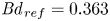 ${\textit {Bd}}_{ref}=0.363$. Note the origin for the parameter space made by the geometry and forcing parameters is indicated by the subscript ‘ref’, while the reference point for the temperature-dependent material properties is denoted by the superscript ‘*’.
Owing its importance for experiments (Majima et al. Reference Majima, Kawamura, Otsubo, Kuwahara and Doi2001; Tanaka et al. Reference Tanaka, Kawamura, Ueno and Schwabe2006; Yano, Hirotani & Nishino Reference Yano, Hirotani and Nishino2018a; Ueno Reference Ueno2021), we consider a liquid bridge made from 2-cSt silicone oil (KF96L-2cs, Shin-Etsu Chemical Co., Ltd., Japan) in air under typical experimental conditions for  $T^* = \bar {T} = 25\,^\circ {\rm C}$. The functions
  $\rho (T)$,
  $\mu (T)$,
  $\lambda (T)$ and
  $c_p(T)$ required in (2.3) can be obtained either through explicitly given correlations or by fitting tabulated data to suitable ansatz functions. The functional dependencies used herein are provided in Appendix A for each property of both the working fluids. Once the continuous functions have been constructed, the reference quantities are evaluated (table 2) and the non-dimensional shape function
  $\alpha _j(T)$ defined in (2.7) are obtained for both phases. Finally, the shape functions are expressed in terms of the reduced temperature:
  $\alpha _j(T)\to \alpha _j(\vartheta )$ such that
  $\alpha _{j}^* = \alpha _j(\vartheta =0)$. For the present liquid–gas couple, the shape functions read
 $$\begin{gather} \alpha_\rho(\vartheta)= \begin{cases} \xi_\text{I}-\xi_\text{II}{\textit{Ca}}\vartheta+\xi_\text{III}{\textit{Ca}}^2\vartheta^2,\\ \dfrac{\zeta_\text{I}}{1+\zeta_\text{II}{\textit{Ca}}\vartheta}, \end{cases} \end{gather}$$
 $$\begin{gather}\alpha_\mu(\vartheta)= \begin{cases} (\xi_\text{I}-\xi_\text{II}{\textit{Ca}}\vartheta+\xi_\text{III}{\textit{Ca}}^2\vartheta^2) \exp[\xi_\text{IV}{\textit{Ca}}\vartheta/(\xi_\text{V}+{\textit{Ca}}\vartheta)] ,\\ \zeta_\text{I}+\zeta_\text{II}{\textit{Ca}}\vartheta+\zeta_\text{III}{\textit{Ca}}^2 \vartheta^2+\zeta_\text{IV}{\textit{Ca}}^3\vartheta^3+\zeta_\text{V}{\textit{Ca}}^4\vartheta^4, \end{cases} \end{gather}$$
 $$\begin{gather}\alpha_\lambda(\vartheta)= \begin{cases} \xi_\text{I}+\xi_\text{II}{\textit{Ca}}\vartheta+\xi_\text{III}{\textit{Ca}}^2\vartheta^2,\\ \zeta_\text{I}+\zeta_\text{II}{\textit{Ca}}\vartheta+\zeta_\text{III}{\textit{Ca}}^2\vartheta^2+\zeta_\text{IV}{\textit{Ca}}^3\vartheta^3+\zeta_\text{V}{\textit{Ca}}^4\vartheta^4, \end{cases} \end{gather}$$
 $$\begin{gather}\alpha_{cp}(\vartheta)= \begin{cases} \xi_\text{I}+\xi_\text{II}{\textit{Ca}}\vartheta+\xi_\text{III}{\textit{Ca}}^2\vartheta^2,\\ \zeta_\text{I}+(\zeta_\text{II}-\zeta_\text{I})G^2(\vartheta)\left[1-F(\vartheta)\left(\zeta_\text{III}+\zeta_\text{IV}G(\vartheta)+\zeta_\text{V}G^2(\vartheta)+\zeta_\text{VI}G^3(\vartheta)\right) \right], \end{cases} \end{gather}$$
where the first line of each subequation specifies the property of the liquid, while the second line represents the property of the gas. The coefficients  $\xi _n$ and
  $\zeta _n$ (
 $n=\text {I},\text {II},\text {III},\ldots$) in (4.1) are constants specific to the respective thermophysical property, and
 \begin{equation} G(\vartheta) = \frac{c_\text{I} +{\textit{Ca}}\vartheta}{c_\text{II}+{\textit{Ca}}\vartheta},\quad F(\vartheta) = \frac{c_\text{II}-c_\text{I}}{c_\text{II}+{\textit{Ca}}\vartheta}, \end{equation}
with  $c_\text {I}=1.14046$ and
  $c_\text {II}=10.89048$. All constant coefficients are collected in tables 3 and 4 for the liquid and gas, respectively. Except for
  $\alpha _{cp}$ for the gas, all coefficients
  $\zeta _\text {I}$ represent the reference quantities, e.g.
  $\zeta _\text {I} = \alpha _\rho ^* = \alpha _\rho (0) = \rho _{g}(25\,^\circ \text {C})/\rho (25\,^\circ \text {C})$.
Table 2. Reference quantities evaluated at  $T^* =25\,^\circ {\rm C}$.
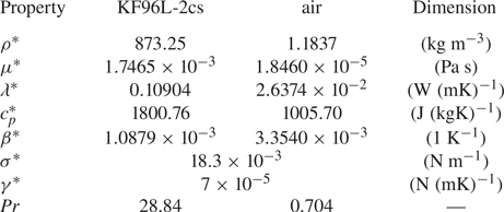
Table 3. Coefficients  $\xi _n$ appearing in the shape functions for 2-cSt silicone oil.

Table 4. Coefficients  $\zeta _n$ appearing in the shape functions for air.

The shape functions  $\alpha _j$ of the four thermophysical parameters for the liquid and gas are shown in figures 2(a) and 2(b), respectively. Shown is the relative variation within each fluid phase of the density, viscosity, thermal conductivity and specific heat capacity as a function of
  $\vartheta$ for a relatively large temperature difference of
  $\Delta T=50$ K. For this temperature difference, most parameters vary almost linearly with a variation of about
  ${\approx }10\,\%$. An exception is the shape function
  $\alpha _\mu$ for the viscosity of the silicone oil (figure 2a). It varies by
  ${\approx }100\,\%$ relative to
  $\alpha _\mu ^*=1$ and has significant nonlinear contributions. This observation indicates the need to take these variations into account.

Figure 2. Normalised shape functions  $\alpha _j/\alpha _{j}^*$ for 2-cSt silicone oil (
 $\alpha _j^*=1$) (a) and for air (b) evaluated at the reference temperature
  $T^*=25\,^\circ {\rm C}$ and for
  $\Delta T=50$ K. The reference parameters
  $\alpha _j^*$ for air are shown as subcaptions in (b).
Ideally, the full temperature dependence of all parameters as shown in figure 2 is taken into account (FTD model). A less demanding approach is the LTD model in which all thermophysical parameters are approximated by linear functions
 \begin{equation} \frac{\alpha_j(\vartheta)}{\alpha_{j}^*} = 1 + \frac{{\alpha'_{j}}^*}{\alpha_{j}^*} \vartheta + O(\vartheta^2) \end{equation}
and terms of  $O(\vartheta ^2)$ are neglected. Within the well-known OB model only the density
  $\rho (\vartheta )$ in the buoyancy term is approximated according to (4.3) while all the other parameters are assumed constant. At times, we also investigate the influence of a single parameter only on the stability boundary, as in Stojanović et al. (Reference Stojanović, Romanò and Kuhlmann2023a), keeping the remaining parameters constant.
A systematic quantification of the variability of the thermophysical parameters has been provided by Stojanović et al. (Reference Stojanović, Romanò and Kuhlmann2023a), in particular their tables 1 and 2. In linear approximation (4.3), a maximum relative deviation of  $c/2$ of a particular thermophysical parameter leads to the requirement
  $(\vartheta \in [-0.5,0.5])$,
 \begin{equation} \left|\frac{{\alpha'_{j}}^*}{\alpha_{j}^{*}}\right| < c. \end{equation}
The most severe restriction on  $\Delta T$ is posed by the viscosity of the liquid. To satisfy (4.4) with
  $c=0.1$ (Gray & Giorgini Reference Gray and Giorgini1976), for instance, restricts the allowable temperature difference to
  $\Delta T = c \mu ^*/(\partial \mu /\partial T)^* \leq 4.8$ K.
5. Results
Originating from the reference values of the geometry and driving parameters (subscript ref) the critical thermocapillary Reynolds number  ${\textit {Re}}_c$ is calculated as a function of the relative volume
  $\mathcal {V}$ of the liquid bridge, the aspect ratio
  $\varGamma$, the size of the system (length scale
  $d$) and the gas flow Reynolds number
  ${Re}_{g}$. These parameters are varied over the following ranges.
(i) The volume ratio is varied within
 ${\mathcal {V}} \in [0.66, 1.3]$ for $\varGamma =\varGamma _{ref}$, ${Re}_{g}={\textit {Re}}_{g,ref}$ and ${\textit {Bd}}={\textit {Bd}}_{ref}$.
(ii) The aspect ratio of the liquid bridge is changed in the range
$\varGamma \in [0.5, 1.8]$ by varying the distance $d$ between the discs for ${\mathcal {V}}={\mathcal {V}}_{ref}$ and ${Re}_{g}={\textit {Re}}_{g,ref}$. The change of $d$ also affects the dynamic Bond number ${\textit {Bd}}\sim d^2$. In order to enable a comparison of the numerical results with laboratory experiments, by varying $d$ we do not keep the dynamic Bond number constant but simultaneously vary ${\textit {Bd}} \in [0.208, 3.70]$ such that ${\textit {Bd}} = {\textit {Bd}}_{ref}(\varGamma /\varGamma _{ref})^2$.(iii) The size of the system is varied by changing
$d \in [0.1, 3]$ mm for $\varGamma =\varGamma _{ref}$, ${\mathcal {V}}={\mathcal {V}}_{ref}$ and ${Re}_{g}={\textit {Re}}_{g,ref}$. As for the variation of $\varGamma$, the dynamic Bond number varies $\sim d^2$ and we vary the Bond number accordingly in the range ${\textit {Bd}} \in [0.016, 1.20]$.(iv) The strength of the gas flow is varied within
${Re}_{g} \in [-3500, 1500]$ for $\varGamma =\varGamma _{ref}$, ${\mathcal {V}}={\mathcal {V}}_{ref}$ and ${\textit {Bd}}={\textit {Bd}}_{ref}$.


While the first, second and fourth variations are often conducted in experiments (see, e.g. Melnikov et al. Reference Melnikov, Shevtsova, Yano and Nishino2015; Yano et al. Reference Yano, Maruyama, Matsunaga and Nishino2016; Gaponenko et al. Reference Gaponenko, Mialdun, Nepomnyashchy and Shevtsova2021), the third variation is intended to reveal the length scale below which the flow in the thermocapillary liquid bridge becomes independent of buoyancy forces under terrestrial conditions.
5.1. Liquid bridge inside a sealed tube
5.1.1. Effect of the volume ratio on the stability boundary
Figure 3 shows the dependence of the critical Reynolds number  ${\textit {Re}}_c$ (a) and frequency
  $\omega _c$ (b) as a function of the volume ratio
  $\mathcal {V}$ taking into account a dynamically deforming interface in the basic flow. Three different flow models are considered: (a) FTD of all parameters (full lines), (b) LTD of all parameters (dashed lines) and (c) the OB approximation (dash-dotted lines). In addition, the black dash-dotted curves are reproduced from Stojanović et al. (Reference Stojanović, Romanò and Kuhlmann2022) who used the OB model, but for slightly different reference parameters and an indeformable, hydrostatic interface according to (2.24) (see § 5.1.2). Note that this line does not distinguish between different wavenumbers. Neutral curves with
  ${\textit {Re}}_n({\mathcal {V}}) > {\textit {Re}}_c({\mathcal {V}})$ slightly above the critical curve are smooth, have similar shapes as
  ${\textit {Re}}_c({\mathcal {V}})$ and typically possess a minimum that is very often larger than the maximum critical Reynolds number arising in figure 3(a). The gross characteristics of the neutral curves for a relatively low Reynolds number and all models considered here, can be inferred from those provided by Stojanović et al. (Reference Stojanović, Romanò and Kuhlmann2022) as functions of
  $\mathcal {V}$,
  $\varGamma$ and
  ${\textit {Bd}}$ in the framework of the OB approximation.

Figure 3. (a) Critical Reynolds number  ${\textit {Re}}_c$ (left side) and critical temperature difference
  $\Delta T_c$ (right side) as functions of the volume ratio
  ${\mathcal {V}}$ for
  $\varGamma =0.66$,
  ${\textit {Bd}}={\textit {Bd}}_{ref}$ and a sealed tube: FTD model (full lines), OB model (dash-dotted lines) and LTD model (dashed lines). The grey-shaded region indicates a deviation of
  $\pm 5\,\%$ from the FTD model. Critical wavenumbers are indicated by colour (see legend). Inserts show zooms into the regions in which
  $m_c=0$. (b) Critical frequencies.
The larger the temperature difference the larger are the deviations among the three models. Based on the usual criterion  $c=0.1$ the OB approximation should be valid only for temperature differences up to
  $\Delta T \leq 4.8$ K (due to the variability of
  $\mu$). Nevertheless, the OB approximation yields critical Reynolds numbers
  ${\textit {Re}}_c$ that deviate less than
  $\pm 5\,\%$ (grey region in figure 3a) from those obtained using the FTD model as long as
  $\Delta T\lesssim 28$ K. The linearised model (LTD, dashed) compares overall better with the FTD model, yet the dashed line (LTD) leaves the grey 5 % tolerance region in the range
  $\mathcal {V}\in [0.752, 0.785]$ at
  $\Delta T\approx 27$ K. The difference in
  ${\textit {Re}}_c$ between the linearised (dashed) and the FTD model (full) becomes more significant in the range
  ${\mathcal {V}} \in [0.842,0.898]$ for
  $\Delta T\gtrsim 45$ K.
The volume ratio  $\mathcal {V}$ has a strong effect on the stability boundary. The slope of
  ${\textit {Re}}_c({\mathcal {V}})$ is particularly large and changes its sign at the peak near
  ${\mathcal {V}}=0.85$. Moreover, the wavenumber and the structure of the critical mode changes along the critical curve. This indicates the value of
  ${\textit {Re}}_c$ is sensitive with respect to small variations of
  ${\mathcal {V}}$ in this region. This sensitivity exists in addition to the sensitivity of
  ${\textit {Re}}_c$ with respect to the model (OB, LTD or FTD) used. For most volume ratios, the critical Reynolds number for the OB model
  ${\textit {Re}}_c^{OB} > {\textit {Re}}_c^{FTD}$ is larger than that of the FTD model that itself is slightly larger than that of the LTD model. To the right of the peak, the critical oscillation frequencies in figure 3(b) exhibit a similar trend as the critical Reynolds number. For lower volume ratios, however, the critical frequencies are much lower.
As an example, we consider  ${\mathcal {V}}=0.88$ (green square in figure 3) for which
  $m_c=3$ for all models. We find that the structure of the basic flow (full and dashed lines in figure 4) and of the respective most dangerous modes (comparison not shown) for all three parameter models are almost identical for
  ${\mathcal {V}}=0.88$. The higher critical Reynolds number for the OB model in comparison to those for the FTD and LTD models in this case might be related to the strong variation of the local viscosity, more precisely, the local kinematic viscosity. Owing to the relatively weak variation of
  $\alpha _\rho$ compared with
  $\alpha _\mu$ (cf. blue and green curve in figure 2a) for the liquid, we focus on the local kinematic viscosity
 \begin{equation} \nu(\vartheta)=\frac{\mu}{\rho}=\frac{\alpha_\mu}{\alpha_\rho}\nu^*. \end{equation}
Its relative deviation from the nominal value  $\nu ^* = 2\times 10^{-6}\ \text {m}^2\ \text {s}^{-1}$ is given by
 \begin{equation} \epsilon_\nu(\vartheta)=\frac{\nu-\nu^*}{\nu^*}=\frac{\alpha_\mu}{\alpha_\rho}-1. \end{equation}
From figure 4(a) the local kinematic viscosity  $\nu$ near the cold wall is larger by more than 60 % than the nominal value, while near the hot wall and the free surface it is more than 20 % smaller than nominal, due to the high surface temperature
  $\vartheta >0$. As a result, the azimuthal perturbation temperature variations associated with the hydrothermal wave lead to larger azimuthal velocity gradients compared with those in the OB model in which the kinematic viscosity on the interface is
  $\nu ^*$, or
  $\epsilon _\nu =0$. Since the azimuthal perturbation velocity drives the hydrothermal wave (Wanschura et al. Reference Wanschura, Shevtsova, Kuhlmann and Rath1995), this effect enhances the velocity field of the critical mode and, thus, may explain the lower critical Reynolds number for the FTD model as compared with the OB model for
  ${\mathcal {V}}=0.88$.

Figure 4. Basic state streamlines (a) and isotherms (b) for  $(\varGamma,{Re}_{g},{\textit {Bd}})=(\varGamma,{Re}_{g},{\textit {Bd}})_{ref}$ and
  $\mathcal {V}=0.88$ at
  ${\textit {Re}}_c=1680$ using the FTD model. In (b) the critical velocity field (arrows) and the critical temperature field (colour) for
  $m_c=3$ is also shown in the (
 $r,z$) plane in which the local thermal production
  $\alpha _{\rho 0}\tilde {\vartheta } \tilde {\boldsymbol {u}} \boldsymbol {\cdot }\boldsymbol {\nabla }\vartheta _0$ takes one of its maxima (white crosses in (a,b) at
  $(r_{max},z_{max})=(1.05,0.19)$). Colour in (a) indicates the local viscosity deviation
  $\epsilon _\nu (\vartheta _0)$. The dashed lines show basic state streamlines and isotherms for the same set of parameters, but using the OB approximation.
The slightly lower critical Reynolds number of the LTD model in comparison to the FTD model for  ${\mathcal {V}}=0.88$ is consistent with the effective kinematic viscosity
 \begin{equation} \nu_{eff}=\left\{ \int_V \rho[T_0(\boldsymbol{x})] \hat {\boldsymbol{u}}^2\,\mathrm{d} V\right\}^{{-}1} \int_V \nu[T_0(\boldsymbol{x})] \rho[T_0(\boldsymbol{x})] \hat {\boldsymbol{u}}^2\,\mathrm{d} V, \end{equation}
which is defined as kinematic viscosity weighted by the kinetic-energy density of the critical mode (see Appendix C). We find that the ordering of the critical Reynolds numbers  ${\textit {Re}}_c^{LTD}<{\textit {Re}}_c^{FTD}<{\textit {Re}}_c^{OB}$ coincides with that of the effective viscosities
  $\nu _{eff}^{LTD}<\nu _{eff}^{FTD}<\nu _{eff}^{OB}$, namely
  $0.853\nu ^*<0.880\nu ^*<\nu ^*$ at the respective critical points of each model. Comparing the three models for a constant Reynolds number at, e.g.
  ${\textit {Re}}={\textit {Re}}_c^{FTD}=1680$ yields the same ordering with
  $0.832\nu ^*<0.880\nu ^*<\nu ^*$.
While the above interpretation seems plausible for  ${\mathcal {V}}=0.88$, this argument cannot generally be proven valid, because the critical curves for the OB approximation and for the FTD model intersect. Thus, for certain ranges of
  ${\mathcal {V}}$, the basic flow is slightly more stable within the FTD model than within the OB model. This indicates that the influence of the changed volume is much more important, not only changing the critical Reynolds number, but also the structure and wavenumber of the critical mode. Regardless of the explanation of the mechanisms at work, the results in figure 3 show that it is important to take into account the variation of the thermophysical parameters (in particular that of the viscosity of the liquid) in order to arrive at accurate critical data when the temperature difference is large, here approximately in the range
  ${\mathcal {V}}\in [0.75, 0.95]$.
In table 5 we compare the critical data obtained for  $\mathcal {V}=0.88$ using different approximations. Within the
  $\text {OB}+\rho (T)$ model, the temperature dependence of the fluid densities is taken into account in all the governing equations (2.4) according to (2.10), whereas the
  $\text {OB}+\mu (T)$ model combines the OB approximation with a FTD dynamic viscosity, while the
  $\text {OB}+\mu _{L}(T)$ model indicates that only the liquid's viscosity is FTD. The
  $\text {OB}+\mu (T)$ and
  $\text {OB}+\mu _{L}(T)$ models yield the smallest deviation of the critical Reynolds number from that of the FTD model. This confirms the importance of taking into account the temperature dependence of
  $\mu (T)$ of the fluids, in particular that of the liquid.
Table 5. Critical Reynolds numbers  ${\textit {Re}}_c$ and critical temperature differences
  $\Delta T_c$ for
  $\mathcal {V}=0.88$ and different model equations (approximations). The relative deviation
  $\epsilon _c=({\textit {Re}}_c - {\textit {Re}}_c^{FTD})/{\textit {Re}}_c^{FTD}$ is given in percent.

5.1.2. Comparison with the results of Stojanović et al. (Reference Stojanović, Romanò and Kuhlmann2022)
Stojanović et al. (Reference Stojanović, Romanò and Kuhlmann2022) have also computed the linear stability boundary  ${\textit {Re}}_c({\mathcal {V}})$ using the OB approximation and the same geometry parameters. However, there are small differences compared with the present investigation: (a) Stojanović et al. (Reference Stojanović, Romanò and Kuhlmann2022) neglected dynamic surface deformations and (b) the reference quantities
  $\alpha _j$ differ slightly; in the present work they are determined by quadratic least-squares fits of the discrete manufacturer's data (cf. § 4), while Stojanović et al. (Reference Stojanović, Romanò and Kuhlmann2022) implemented the discrete values specified for the reference temperature, except for the thermal expansion coefficient that was taken from Romanò et al. (Reference Romanò, Kuhlmann, Ishimura and Ueno2017), because it is not contained in the data sheet provided by the manufacturer.
Tests have shown that the dynamic surface deformation  $\Delta h_0=h_{0,d}-h_{0,s}$ in the basic flow, where
  $h_{0,d}$ and
  $h_{0,s}$ are the dynamic and static surface shapes, respectively, has a weak influence on the critical Reynolds number near the peak of
  ${\textit {Re}}_c(\mathcal {V})$ at
  ${\mathcal {V}} \approx 0.9$. For these volume ratios, differences between the present results using the OB approximation and those of Stojanović et al. (Reference Stojanović, Romanò and Kuhlmann2022) are mainly due to the different reference values
  $\alpha _j$ used, in particular due to the difference in
  $\beta ^*$ for the liquid phase: Stojanović et al. (Reference Stojanović, Romanò and Kuhlmann2022) used the same value for
  $\beta ^*$ as did Romanò et al. (Reference Romanò, Kuhlmann, Ishimura and Ueno2017). This value is 11.4 % larger than the current value used (table 2). The impact is visible from figure 3, where the critical Reynolds number obtained by Stojanović et al. (Reference Stojanović, Romanò and Kuhlmann2022) (black dash-dotted line) significantly deviates from the current result using the OB approximation (coloured dash-dotted line) for
  $\mathcal {V}\lesssim 1$. In particular, an axisymmetric
  $m=0$ mode is critical in the present investigation in the narrow range
  ${\mathcal {V}} \in [0.8663, 0.8712]$ (brown dash-dotted line, upper inset of figure 3a), whereas the axisymmetric critical mode arises for
  ${\mathcal {V}} \in [0.8917,8983]$ in Stojanović et al. (Reference Stojanović, Romanò and Kuhlmann2022) (full black line in their figure 17a). The different thermophysical reference parameters are also responsible for the significant reduction of the volume ratio range within which the wavenumber
  $m=4$ is critical:
  ${\mathcal {V}} \in [0.871,0.874]$ (orange dotted line in figure 3a) as compared with
  ${\mathcal {V}} \in [0.898,0.929]$ (full purple line in figure 17(a) of Stojanović et al. Reference Stojanović, Romanò and Kuhlmann2022). The changes indicate the sensitivity of the critical Reynolds number on the thermophysical reference parameters
  $\alpha _j$, not only for the OB approximation but in general.
5.1.3. Effect of the aspect ratio on the stability boundary
The aspect ratio  $\varGamma =d/r_\text {i}$ can easily be adjusted in experiments and is an important parameter determining the critical wavenumber. Therefore, we vary the length
  $d$, as in experiments, keeping
  $r_{i} = r_{i,ref}$ constant. The Bond number is adjusted accordingly
  ${\textit {Bd}}={\textit {Bd}}_{ref}\times (\varGamma /\varGamma _{ref})^2$. The dependence of the critical conditions on
  $d$ is displayed in figure 5(a), where the critical Reynolds number
  ${\textit {Re}}_c$ is shown as a function of the aspect ratio
  $\varGamma$ for
  $\mathcal {V}=1$ and the three models employed (OB, LTD, FTP). Figure 5(b) shows the corresponding critical frequencies. While the critical frequencies increase with the critical Reynolds number to the left of the peak of
  ${\textit {Re}}_c$ (small
  $\varGamma$), the opposite behaviour is found for the frequency of the critical
  $m=1$ mode to the right of the peak of
  ${\textit {Re}}_c$ (larger
  $\varGamma$). In addition, we reproduce in figure 5
  ${\textit {Re}}_c(\varGamma )$ and
  $\omega _c(\varGamma )$ (black dash-dotted curves) obtained by Stojanović et al. (Reference Stojanović, Romanò and Kuhlmann2022) for the OB model, but for slightly different reference parameters and an indeformable interface. Since, for the present parameter variation,
  $\Delta T_c \sim {\textit {Re}}_c/d$ scales differently from
  ${\textit {Re}}_c$, straight grey lines in 5(a) refer to constant values of
  $\Delta T$.

Figure 5. (a) Critical Reynolds number  ${\textit {Re}}_c$ (left axis) and critical temperature difference
  $\Delta T_c$ (right axis) as functions of the aspect ratio
  $\varGamma$ for
  $\mathcal {V}=1$,
  ${\textit {Bd}}={\textit {Bd}}_{ref}\times (\varGamma /\varGamma _{ref})^2$ and a closed chamber. The curves related to the left and right vertical axis, respectively, are indicated by the additional label in the right corner of the graph. Results are shown for FTD (full lines), LTD (dashed lines) and OB (dash-dotted lines) models. The grey shaded region indicates a deviation of
  $\pm 5\,\%$ from the reference FTD model. (b) Critical frequencies.
For most aspect ratios, all present critical Reynolds numbers lie within the 5 % tolerance level about the result for the FTD model (full line). However, similarly as for the variation of  $\mathcal {V}$ above, the OB model (coloured dash-dotted lines) overestimates the critical Reynolds number by more than 5 % in the range
  $\varGamma \in [0.806,1.086]$. The sensitivity of the critical Reynolds number on the reference parameters
  $\alpha _j$ is again confirmed when comparing the OB model of Stojanović et al. (Reference Stojanović, Romanò and Kuhlmann2022) (black dash-dotted line) with the current OB model results (coloured dash-dotted line). In Stojanović et al. (Reference Stojanović, Romanò and Kuhlmann2022) buoyancy forces have been overestimated due to the larger selected
  $\beta ^*$. This also explains the increasing discrepancy of
  ${\textit {Re}}_c$ for long liquid bridges (large
  $\varGamma$). Numerical tests have shown that including dynamic surface deformations in the model of Stojanović et al. (Reference Stojanović, Romanò and Kuhlmann2022) have only a very minor effect on the black dash-dotted curves. The comparison thus underlines that the selection of the reference quantities (here
  $\beta ^*$) has a profound effect on
  ${\textit {Re}}_c$ that can be large when the slope of
  ${\textit {Re}}_c(\varGamma )$ is large.
As a minor detail, the OB approximation predicts the critical wavenumber  $m_c=2$ (red) within a very small window of
  $\varGamma$ at the peak of
  ${\textit {Re}}_c$ (inset of figure 5a), whereas the FTD model yields
  $m_c=3$ (green). Likewise, the critical mode with
  $m_c=2$ does not arise in the OB model used by Stojanović et al. (Reference Stojanović, Romanò and Kuhlmann2022), but from their calculations neutral modes with different wavenumbers arise at very close Reynolds numbers near the peak of
  ${\textit {Re}}_c(\varGamma )$.
Close to the peak of  ${\textit {Re}}_c$ that coincides with a maximum of the critical temperature difference, the distribution of the kinematic viscosity
  $\nu (\boldsymbol {x})$ exhibits a similar structure as for
  $(\varGamma,{Re}_{g},{\textit {Bd}})=(\varGamma,{Re}_{g},{\textit {Bd}})_{ref}$ and
  $\mathcal {V}=0.88$. This is evident when comparing figure 6(a) for
  $\varGamma =0.93$ (green square in figure 5) with figure 4(a). Despite the quantitative differences of
  $\nu$, the effective viscosities based on the result for
  ${\textit {Re}} = {\textit {Re}}_c^{FTD}(\varGamma =0.93) = 1438$ are ordered with
  $\nu _{eff}^{LTD}=0.911 < \nu _{eff}^{FTD}=0.923 < \nu _{eff}^{OB}=1$, just like the Reynolds numbers are
  $({\textit {Re}}_c^{LTD}<{\textit {Re}}_c^{FTD}<{\textit {Re}}_c^{OB})$. The impact of the effective viscosity is demonstrated in figure 6(b), where the basic state isotherms of the FTD model (full black lines) are compared with those obtained by the OB model (dashed black lines) at the same Reynolds number
  ${\textit {Re}}={\textit {Re}}_c^{FTD}=1438$. At this Reynolds number the most dangerous mode of the OB model (not shown) is linearly stable. The slightly stronger basic flow in the FTD model compared with the OB model (cf. dashed and full white lines in figure 6a) yields a slightly stronger basic state thermal advection (cf. dashed and full black isotherms in figure 6b). This enhances the energy supply from the basic state to the perturbation flow, which destabilises the flow.

Figure 6. Same as figure 4 but for  $(\mathcal {V},{Re}_{g})=(\mathcal {V},{Re}_{g})_{ref}$,
  $\varGamma =0.93$ and
  ${\textit {Re}}_c=1438$.
5.1.4. Effect of the length scale on the linear stability boundary
The size of a liquid bridge, parameterised by the length scale  $d$, is perhaps the most important design parameter for experiments. It affects the static shape of the liquid bridge through the hydrostatic pressure difference and determines its mechanical stability (see, e.g. Meseguer, Slobozhanin & Perales Reference Meseguer, Slobozhanin and Perales1995). Apart from these mechanical aspects, the size affects the critical thermocapillary Reynolds number, because (a) the strength of buoyancy forces to thermocapillary forces depends on size, and (b) the range of variation of the material parameters depends on size through the size dependence of the critical temperature difference.
To investigate these influence factors, we consider  $\varGamma =0.66$,
  $\varGamma _{s}=0.4$,
  $\eta =4$,
  ${\mathcal {V}}=1$ and take into account the dynamic surface shape of the liquid bridge in the basic state. While the FTD model is the most realistic one, it is instructive to compare the size dependence of the critical Reynolds number of the different models with the OB approximation under zero gravity conditions (OB-0g). For zero gravity and in the absence of a forced gas flow, deviations of the shape from cylindrical are only due to the basic flow (DI). If dynamic deformations are suppressed (SI), the length scale and the temperature difference would only appear in the Reynolds number
  ${\textit {Re}} \sim \Delta T d$. Therefore, the stability boundary for the OB-0g model and a SI is simply
  ${\textit {Re}}_c(d) = 627 = \text {const.}$ with
  $\Delta T_c\sim d^{-1}$. In the present case of a DI the effect of the dynamic surface deformation in the basic state only becomes relevant for small values of
  $d$, thus large values of
  $\Delta T_c$, because a high temperature difference significantly increases the capillary number entering the normal stress balance (2.20a), which makes the interface more deformable dynamically. The effect is visible in figure 7 by the minute reduction of
  ${\textit {Re}}_c^\text {OB-0g}$ (black curve, DI) from
  ${\textit {Re}}=627$ (SI) for
  $d\lesssim 0.25$ mm. The critical wavenumber for the case OB-0g is
  $m_c=2$ in the full range of
  $d$ investigated.

Figure 7. Critical Reynolds number as a function of the size of the set-up expressed through  $d$ for constant geometrical proportions
  $\varGamma =0.66$,
  $\varGamma _{s}=0.4$,
  $\eta =4$ and
  ${\mathcal {V}}=1$. Different gravity conditions and flow models are considered (see the legend). The grey hatched region corresponds to inaccessible critical temperature differences with
  $\Delta T_c >126$ K. The grey shaded region indicates a deviation of 5 % from the zero gravity reference case (blue lines). Full lines: critical Reynolds numbers. Dashed line: neutral Reynolds numbers close to the intersection of critical curves. The wavenumber
  $m$ is given for each segment of the critical curve.
The critical Reynolds number  ${\textit {Re}}_c^\text {OB-0g}(d)$ for OB-0g represents the reference. The grey strip indicates a
  ${\pm }5\,\%$ deviation from
  ${\textit {Re}}_c^\text {OB-0g}$. The effect of the terrestrial gravity level and of the full temperature dependence of the material parameters on the critical Reynolds number when the length scale
  $d$ is varied is shown in figure 7 for the OB and FTD models and for 0g and 1g.
In the framework of the OB approximation (OB-1g) the buoyancy force in the liquid phase in (2.4) becomes in our scaling
 \begin{equation} {-}{\textit{Bd}}\frac{\alpha_\rho-\alpha_{\rho}^{*}}{\varepsilon} = \frac{\rho^*g\beta^*d^2}{\gamma^*}\vartheta = \frac{U_{diff}}{U_{TC}} {\textit{Ra}}\vartheta, \end{equation}
where  $U_{diff}=\lambda ^*/(\rho ^* c_p^* d)$ and
  $U_{TC}=\gamma ^*\Delta T/\mu ^*$ are the characteristic velocity scales for thermal diffusion in the liquid and for thermocapillary convection, respectively, and
 \begin{equation} {\textit{Ra}} = \frac{g\beta^*\Delta T d^3}{(\lambda^*/\rho^*c_p^*)(\mu^*/\rho^*)} \end{equation}
is the Rayleigh number. Due to the dependence  ${\textit {Ra}}\sim d^3$, buoyancy forces rapidly diminish in the liquid phase as the length scale
  $d$ is reduced and if approximately
  $\Delta T \sim d^{-1}$. Therefore, the critical Reynolds number
  ${\textit {Re}}_c$ under terrestrial gravity within the OB approximation (OB-1g, green in figure 7) approaches the zero gravity case (OB-0g, black) in the limit of vanishing
  $d$. As
  $d$ increases beyond
  $d \approx 0.4$ mm, the basic flow first becomes slightly stabilised due to buoyancy within the OB-1g model. The change of the critical wavenumber from
  $m_c=2$ to
  $m_c=3$ at
  $d=0.65$ mm leads to a slight reduction of the critical Reynolds number below that for the case OB-0g until, for
  $d\gtrsim 1.6$ mm, buoyancy forces again strongly stabilise the basic flow. Further increasing
  $d$ the critical Reynolds number grows significantly and a more complicated switching of critical modes arises. Based on the OB approximation, the influence of buoyancy forces on the critical Reynolds number for the present couple of fluids and geometry remains less than
  ${\approx }4.5\,\%$ as long as
  $d<1.6$ mm. A relation similar to (5.4) holds for the buoyancy force in the gas phase. However, the Rayleigh number would not scale like
  ${\sim }d^3$ for the present parameter variation with constant values of
  $\varGamma _{s}$ and
  $\eta$.
The picture changes when the full temperature dependence of the material parameters are taken into account. Under zero gravity, the FTD model (FTD-0g, blue) yields a critical Reynolds number larger than  ${\textit {Re}}_c^\text {OB-0g}$ for
  $d\gtrsim 0.37$ mm. Figure 8 shows the critical mode using the FTD-0g model (a) and the OB-0g model (b) for
  $d=1$ mm. The isotherms of the basic state (black lines) indicate again a higher temperature close to the free surface for FTD-0g. However, in contrast to the case shown in figure 4, the FTD-0g model is more stable than the OB-0g model, i.e.
  ${\textit {Re}}_c^\text {FTD-0g} > {\textit {Re}}_c^\text {OB-0g}$. This finding is consistent with figure 3 (for
  $\mathcal {V}=1$) in the presence of buoyancy forces.

Figure 8. Linear stability results for  $(\mathcal {V},\varGamma,{Re}_{g})=(\mathcal {V},\varGamma,{Re}_{g})_{ref}$,
  ${\textit {Bd}}=0$ and
  $d=1$ mm using the FTD model (a) and the OB model (b). Shown are the critical velocity field (arrows) and critical temperature field (colour) in the (
 $r,z$) plane in which the local production
  $\alpha _{\rho 0}\tilde {\vartheta }\tilde {\boldsymbol {u}}\boldsymbol {\cdot }\boldsymbol {\nabla }\vartheta _0$ takes one of its maxima (white crosses) in the bulk. Black lines indicate isotherms of the basic state. Results are shown for (a)
  ${\textit {Re}}_c=676$,
  $m_c=2$; (b)
  ${\textit {Re}}_c=627$,
  $m_c=2$.
The difference between OB-0g and FTD-0g vanishes asymptotically as  $d$ becomes larger, because the critical temperature difference decreases
  ${\sim }d^{-1}$, provided
  ${\textit {Re}}_c\approx \text {const}$. Therefore, the material properties hardly vary anymore within their respective domains. This also becomes clear when taking the limit
  $\Delta T\to 0$ in (2.7) in which the shape functions for the liquid reduce to
  $\alpha _j\equiv 1$. Asymptotically,
  ${\textit {Ca}}\sim d^{-1}$ such that the Laplace pressure dominates and the liquid bridge takes a perfect cylindrical shape. If, on the other hand, the size of the bridge is reduced, the critical wavenumber for the FTD-0g model changes from
  $m_c=2$ to
  $m_c=3$ at
  $d=0.84$ mm. For even smaller sizes, the basic flow is strongly destabilised for
  $d< 0.25$ mm within the FTD-0g model. This effect is due to the increased range of variation of the material properties when the critical temperature difference increases due to the reduction of the length scale. In this region (grey hatched in figure 7) other effects like evaporation become important that are not taken into consideration here. In any case, the maximum theoretical temperature difference is bounded by the pour point and the boiling temperature that, for 2-cSt silicone oil, are
  $-120\,^\circ {\rm C}$ and
  $88\,^\circ {\rm C}$, respectively. The latter restricts the experimentally realisable temperature differences to
  $\Delta T < 2\times (88-25)\,^\circ \text {C} = 126\,^\circ {\rm C}$, assuming that the mean temperature is kept at
  $25\,^\circ {\rm C}$. Temperature differences above this threshold fall into the grey hatched region.
For small length scales  $0.35\ \text {mm}\leq d\lesssim 0.5$ mm, deviations of
  ${\textit {Re}}_c$ from the reference case
  ${\textit {Re}}_c^\text {OB-0g}$ are primarily caused by the temperature dependence of the material properties and not by either buoyancy or dynamic deformations of the interface. Therefore, the critical Reynolds number under terrestrial gravity conditions for the FTD model (FTD-1g, red) hardly deviates from
  ${\textit {Re}}_c$ under zero gravity (FTD-0g, blue) for
  $d\lesssim 0.5$ mm with
  $m_c=3$. For larger system sizes, the critical Reynolds number for FTD-1g remains closer to the results for OB-0g and OB-1g and the critical wavenumber
  $m_c=3$ for the FTD-1g model does not change before
  ${\textit {Re}}_c$ for the terrestrial conditions (red, green) starts increasing strongly from the 0g cases (black, blue) for
  $d\gtrsim 1.6$ mm.
In summary, the critical data ( ${\textit {Re}}_c$ and
  $m_c$) under terrestrial gravity modelled by the FTD-1g model (red) is comparable (up to 5 %) to the OB-1g model (green) as long as
  $d\geq 0.69$ mm. For smaller lengths, the OB-1g model yields a different critical wavenumber
  $m_c$. For zero gravity conditions, the critical Reynolds numbers of the FTD-0g model (blue) can be predicted by the simpler OB-0g model (black) with an accuracy better than 5 % if
  $d\leq 1.64$ mm. Moreover, in the range
  $d\in [0.35,1.5]$ mm, all four models yield comparable results since
  ${\textit {Re}}_c$ is almost constant and bounded by
  ${\textit {Re}}_c\in [615,683]$. It is remarkable that, for
  $d\geq 1.64$ mm, the large critical Reynolds numbers and the mode switching leading to the peak of
  ${\textit {Re}}_c$ for the OB-1g and FTD-1g models are essentially caused by the increasing buoyancy forces in the bulk when heating from above and by the increasing static shape deformation
  $({\textit {Bo}}\sim d^2)$. Dynamic deformation are of minor importance for increasing
  $d$, indicated by the small deviation of
  ${\textit {Re}}_c^\text {OB-0g}$ (black in figure 7) from the constant value
  ${\textit {Re}}_c^\text {OB-0g,SI}=627$.
5.2. Effect of temperature-dependent thermophysical properties in the presence of an axial gas flow
A concentric circular tube about the liquid bridge, originally designed to minimise ambient air effects on the flow in the liquid, can be utilised to impose an axial flow in the gas phase that bears some potential to control the onset of a time-dependent and/or three-dimensional flow in the liquid phase (Shevtsova, Gaponenko & Nepomnyashchy Reference Shevtsova, Gaponenko and Nepomnyashchy2013; Shevtsova et al. Reference Shevtsova, Gaponenko, Kuhlmann, Lappa, Lukasser, Matsumoto, Mialdun, Montanero, Nishino and Ueno2014; Yano et al. Reference Yano, Maruyama, Matsunaga and Nishino2016, Reference Yano, Nishino, Ueno, Matsumoto and Kamotani2017; Yasnou et al. Reference Yasnou, Gaponenko, Mialdun and Shevtsova2018; Stojanovic & Kuhlmann Reference Stojanović and Kuhlmann2020; Gaponenko et al. Reference Gaponenko, Mialdun, Nepomnyashchy and Shevtsova2021). Following Stojanovic et al. (Reference Stojanović, Romanò and Kuhlmann2023), we impose an axial gas flow at the inlet of the annular space around the liquid bridge. The velocity profile  $w_{g,in}(r)$ is fully developed according to (2.29) and its strength is measured by the gas flow Reynolds number
  ${Re}_{g}=\bar {W}_{g,in}\rho ^*d/\mu ^*$ as defined in Stojanovic et al. (Reference Stojanović, Romanò and Kuhlmann2023). The gas at the inlet has a homogeneous temperature corresponding to that of the adjacent support disc. Thus, for an upward flow with
  ${Re}_{g}>0$, the gas is cold
  $(\vartheta _{0,{in}}=-0.5)$, while for a downward flow with
  ${Re}_{g}<0$, it is hot
  $(\vartheta _{0,{in}}=0.5)$.
Critical Reynolds numbers  ${\textit {Re}}_c$ and frequencies
  $\omega _c$ as functions of the gas flow Reynolds number
  ${Re}_{g}$ are shown in figure 9(a,b) for the FTD (solid), LTD (dashed) and OB model (dash-dotted line). The sensitivity of the critical Reynolds number with respect to the gas flow for small values
  $|{Re}_{g}|\lesssim 50$ has been explained by Stojanovic et al. (Reference Stojanović, Romanò and Kuhlmann2023). The critical curves for all models behave qualitatively similar as reported in figure 2(a) of Stojanovic et al. (Reference Stojanović, Romanò and Kuhlmann2023) for an extended OB model that almost agrees with the current standard OB model. Also for upward flow
  $({Re}_{g}\gtrsim 50)$ and strong downward flow
  $({Re}_{g}\lesssim -2000)$, the critical Reynolds numbers are almost independent of
  ${Re}_{g}$ and in the range of
  ${\textit {Re}}_c\approx 400$. For these conditions, the three models yield comparable results well within the 5 % tolerance margin (grey). However, for downward flow in the intermediate range of
  $-2000 \lesssim {Re}_{g} \lesssim -50$, the three material parameter models yield very different results (table 6). This is due to the large critical temperature difference for which the dependence of the thermophysical parameters on the flow becomes important.

Figure 9. Left panels: (a) critical Reynolds number  ${\textit {Re}}_c$ (black axis labels) and critical temperature difference
  $\Delta T_c$ (purple axis labels) and (b) critical frequencies as functions of the gas flow Reynolds number
  ${Re}_{g}$ for
  $\varGamma =0.66$,
  $\mathcal {V}=1$ and
  ${\textit {Bd}} = {\textit {Bd}}_{ref}$. Results are shown for the FTD model (full lines), the LTD model (dashed lines) and the OB approximation (dash-dotted lines). The grey-shaded region indicates a deviation of
  $\pm 5\,\%$ from the reference FTD model. The wavenumbers are coded by colour. Right panels: (a) full neutral Reynolds numbers and (b) neutral frequencies for individual wavenumbers.
Table 6. Critical Reynolds number  ${\textit {Re}}_c$ and critical temperature difference
  $\Delta T_c$ for
  ${Re}_{g}=-1500$,
  ${Re}_{g}=-500$ and
  ${Re}_{g}=-250$. Results are given for different approximations. The relative deviation
  $\epsilon _c=({\textit {Re}}_c - {\textit {Re}}_c^{FTD})/{\textit {Re}}_c^{FTD}$ is given in percent.

The critical Reynolds numbers obtained using the OB approximation (dash-dotted line) are typically much larger in the range  $-2000 \lesssim {Re}_{g} < -50$ than the reference data for FTD. An exception is the
  $m=1$ OB mode that is responsible for a local minimum
  ${\textit {Re}}_c^{OB}(m=1)=1727$ of the critical Reynolds number at
  ${Re}_{g}=-480$. Within
  ${Re}_{g}\in [-767,-345]$ the critical Reynolds number for the OB model is even slightly less than that for the FTD model,
  ${\textit {Re}}_c^{OB} < {\textit {Re}}_c^{FTD}$. Despite similar critical Reynolds numbers near
  ${Re}_{g}=-480$, the wavenumbers, oscillation frequencies and flow structures of the critical modes of the two models differ. The linear LTD model (dashed) represents a better approximation to the FTD model (full) than the OB model (dash-dotted line). Like for the FTD model, the critical curve
  ${\textit {Re}}_c^{LTD}({Re}_{g})$ is unique and has the same shape as
  ${\textit {Re}}_c^{FTD}({Re}_{g})$. However, the LTD model underestimates the critical threshold by more than 10 % in the range
  ${Re}_{g}\in [-1705,-32]$. Noteworthy, there exists a considerable range of
  ${Re}_{g}$ around
  ${Re}_{g}\approx -500$ in which the most dangerous mode of the FTD model is axisymmetric (brown line). Furthermore, a critical mode with wavenumber
  $m_c=4$ can be critical within the FTD model, but not for the other models.
The larger critical Reynolds numbers for the OB model (except for the  $m=1$ mode) and the smaller ones for the LTD model as compared with
  ${\textit {Re}}_c^{FTD}$ are caused by the considerable viscosity variation for large
  $\Delta T$. For most values of
  ${Re}_{g}$, we find the effective kinetic-energy-weighted viscosity (5.3) is ordered like
  $\nu _{eff}^{LTD} < \nu _{eff}^{FTD} < \nu _{eff}^{OB}$. Therefore, it is reasonable to assume that the perturbation flow experiences the most dissipation for the OB model and the least for the LTD model. But also the magnitude of the streamfunction extrema of the basic flows for a constant Reynolds number
  ${\textit {Re}}=1500$ provided in table 7 show the same ordering. Thus, a higher Reynolds number is required in the OB model to establish the characteristic internal temperature gradients by advection, from which the hydrothermal wave can draw its thermal perturbation energy. This effect is assisted by the lower surface temperature in the OB model as compared with the FTD model at the same thermocapillary Reynolds number as shown in figure 10.

Figure 10. Tangential velocity  $u_{t0}=\boldsymbol {t}\boldsymbol {\cdot } \boldsymbol {u}_0$ (blue) and temperature distribution
  $\vartheta _0$ (red) of the basic flow along the free surface (parameterised by
  $z$) for
  $({Re}_{g},{\textit {Re}}) = (-1500,1616)$. The models FTD, LTD and OB are distinguished by line type (see legend). The insets show the velocity peaks near the hot and cold corners.
Table 7. Scaled streamfunction extrema  $|\check {\psi }_{min}|=|\psi _{min}|\times 10^3$ of the basic flow and effective viscosities
  $\nu _{eff}$ for
  ${\textit {Re}}=1500$ and different
  ${Re}_{g}$ for the three models LTD, FTD and OB.

Figure 11 shows the most important integral thermal energy production terms  $J_1$ (blue) and
  $J_2$ (red) for the FTD model as functions of the gas flow Reynolds number. We note the heat transfer through the interface is always negligible compared with the bulk thermal production rates
  $J_1$ and
  $J_2$, since
  $-1.3\times 10^{-3}< H_{fs}<0$. For
  ${Re}_{g} < -1750$ and for
  ${Re}_{g} > 0$, the critical Reynolds number is low and the thermal perturbation energy is almost entirely provided by radial advection of the basic state temperature described by the term
  $J_1$ (blue). The variation of the relative importance of
  $J_1$ and
  $J_2$ indicates changes of the model structure or the critical wavenumber. The changes of the critical mode along
  ${\textit {Re}}_c({Re}_{g})$ are illustrated in the supplementary movie for the FTD model available at https://doi.org/10.1017/jfm.2023.998. For strong downward flow of the hot gas
  $({Re}_{g}=-3500)$, the region of basic state temperature gradients (full black lines) is located at about one half of the radius of the liquid bridge
  $(r \approx 1/2\varGamma )$. The temperature perturbation spots extend from top to bottom and the perturbation flow arises in the form of six vortices (
 $m=3$) that are almost aligned with the
  $z$ axis. In this region the temperature perturbation spots are almost exclusively created by the radial perturbation flow such that
  $J_1\approx 1$ and
  $J_2\approx 0$. By increasing
  ${Re}_{g}$ from
  $-1750$ to
  $-1500$ the basic flow becomes more stable (figure 9a). Due to the larger critical temperature difference at the critical point the hot fluid transported along the free surface downward to the cold end of the bridge has an increasing tendency to rise due to buoyancy. As a result, the basic state temperature gradients move closer to the interface and become thinner. This is accompanied with a structural change of the critical mode (see also figure 11) such that the temperature perturbations increasingly spiral about the axis. In the cross-section shown in the movie this is visible by the temperature spots of alternating sign that seem to grow out of the cold corner as
  ${Re}_{g}$ increases.

Figure 11. Normalised thermal perturbation energy production rates  $J_1$ (blue) due to radial advection and
  $J_2$ (red) due to axial advection in the liquid phase according to (3.10b) as functions of
  ${Re}_{g}$ along the critical curve of the FTD model (full lines in figure 9a). The vertical dotted lines indicate changes of the critical wavenumber
  $m_c$ as indicated.
In the plateau region of  ${\textit {Re}}_c$, approximately for
  ${Re}_{g}\in [-1500,-300]$, the basic temperature field does not change much. But the critical wavenumber changes monotonically from
  $m=3$ to
  $m=0$. With each reduction of
  $m$ the importance of
  $J_2$ (axial advection) over
  $J_1$ grows (figure 11). Due to the radially quite localised basic state temperature gradients also the critical modes are confined to this radial region. The radial confinement of the critical modes may explain why the azimuthal wavenumber (if not too large) is not very important for the instability such that the segments of the critical curve in figure 9(a) merge relatively smoothly. In the range
  ${Re}_{g}\in [-300,230]$, the perturbation temperature spots widen again radially owing to the decreasing basic state temperature gradients such that for
  ${Re}_{g} \gtrsim 230$ the perturbation mode resembles the mode for
  ${Re}_{g} \lesssim -1750$. This is due to the reduced heating from the free surface (even cooling for
  ${Re}_{g} > 0$) and a reduction of the buoyant rise of the return flow in the bulk.
We shall now focus on the region between  ${Re}_{g} \approx \in [-2000, 0]$, where most of the deviations between the OB, LTD and FTD models are observed. For a given
  ${Re}_{g}$, the basic flow structure remains qualitatively very similar upon a change of the model (either OB, LTD or FTD), however, the critical thermocapillary Reynolds number can be significantly different. The difference in
  ${\textit {Re}}_c$ between the FTD and LTD model can be explained via the effective viscosity for all modes, except for the
  $m=1$ mode of the OB model. In this sense the
  $m=1$ OB mode is atypical and has a much lower frequency than all other modes. To investigate more in depth the difference between the OB
  $m=1$ instability and the peculiar plateau of the critical stability curve for the FTD and LTD models, figures 12 and 13 compare the basic state isotherms (lines) and the perturbation velocity (arrows) and temperature (colour) fields of the OB for
  $m=1$ and the FTD model for
  $m=0$ (at criticality) and for
  $m \in [1, 4]$ at
  ${Re}_{g} = -500$ and
  ${\textit {Re}} = {\textit {Re}}_c = 1853$ (brown square in figure 9a). It is observed that the most dangerous mode for the OB model
  $(m=1)$ is qualitatively different from the other modes observed for the FTD perturbations. The most dangerous
  $m=1$ mode of the OB model is promoted by a radially narrow perturbation vortex near the top right corner of the liquid bridge. This cannot well exploit the basic state temperature gradient, hence, it requires a perturbation temperature developed over a thicker annular region in order to produce enough energy to feed the
  $m_c=1$ hydrothermal wave perturbation (see figure 12f). On the other hand, for FTD (as well as for LTD, not shown), the velocity perturbation is strongest where the basic state temperature gradient is most intense. This allows the most dangerous perturbation to concentrate its temperature peaks in a thin toroidal blade (see figure 12a–e). The radial confinement of the temperature perturbation is illustrated by the green lines in figures 12 and 13 indicating the projection of the isosurfaces
  $\tilde {\vartheta }=0.5\times \text {max}(\tilde {\vartheta })$ onto the respective planes. As the radial extension of the production region for FTD and LTD (not shown) is relatively small, the instability mechanism becomes almost insensitive to the perturbation wavenumber. This explains the plateau of the neutral stability curves (see panels on the right of figure 9) for the FTD and LTD models, that signifies that the flow in the liquid bridge can be driven towards an unstable state at
  ${\textit {Re}} \approx 1850$ for FTD and
  ${\textit {Re}} \approx 1700$ for LTD for all azimuthal wavenumbers
  $m$ considered. The supplementary movie confirms this interpretation.

Figure 12. Basic state isotherms (black lines), perturbation temperature field (colour) and perturbation velocity field (arrows) in the plane  $\varphi =\text {const.}$ in which the local thermal production
  $\alpha _{\rho 0}\tilde {\vartheta } \tilde {\boldsymbol {u}} \boldsymbol {\cdot } \boldsymbol {\nabla } \vartheta _0$ is maximised (white crosses). Shown are (a) the critical mode with
  $m=0$ of the FTD model for
  $(\mathcal {V},\varGamma,{\textit {Bd}})=(\mathcal {V},\varGamma,{\textit {Bd}})_{ref}$,
  ${Re}_{g}=-500$ and
  ${\textit {Re}}_c=1853$ (brown square in figure 9a). Also shown for the same parameters are the stable modes with
  $m=1$ to
  $m=4$, in (b–e), and the unstable most dangerous mode with
  $m=1$ for the OB model in (f). The dashed black lines indicate horizontal cuts shown in figure 13. The green lines represent the isosurfaces
  $\tilde {\vartheta }= 0.5\times \max (\tilde {\vartheta })$ projected onto the respective plane.

Figure 13. Same as figure 12 but for constant  $z$. The grey arrows indicate the direction of propagation of the mode. Results are shown for (a)
  $m=0$ (FTD), (b)
  $m=1$ (FTD), (c)
  $m=2$ (FTD), (d)
  $m=3$ (FTD), (e)
  $m=4$ (FTD) and (f)
  $m=1$ (OB).
6. Discussion and conclusions
The linear stability of a differentially heated thermocapillary liquid bridge has been investigated numerically. Three distinct models were analysed for a silicone oil liquid bridge in air: the OB approximation, a LTD of all material properties and a full nonlinear dependence of all material parameters on temperature (FTD). The critical stability curves have been computed as functions of the volume ratio  $\mathcal {V}$ of the liquid bridge, its aspect ratio
  $\varGamma$, its size
  $d$ and for a forced axial flow in the surrounding air measured by
  ${Re}_{g}$. The OB approximation tends to overestimate the critical Reynolds number, while the linear model underestimates it. This trend can be explained by an effective viscosity
  $\nu _{eff}$, because the viscosity is by far the most temperature-dependent material property. If the effective viscosity rules the critical onset, then the modified Reynolds number of the FTD model
  $(\nu ^*/\nu _{eff})^2{\textit {Re}}_c^{FTD}\approx {\textit {Re}}_c^{OB}$ should be comparable to that of the OB model. This correlation holds true approximately if
  $\nu _{eff}$ is defined as the perturbation kinetic-energy-weighted kinematic viscosity of the FTD model at criticality. Defining
  $\nu _{eff}$ this way was found to be more suitable than the surface-averaged viscosity proposed by Kozhoukharova et al. (Reference Kozhoukharova, Kuhlmann, Wanschura and Rath1999), because the surface-averaged viscosity only accounts for the driving of the basic and perturbation velocity fields, but does not take care of the thermal perturbation energy production of the hydrothermal wave due to the advection across basic state temperature gradients in the bulk. Unlike Kozhoukharova et al. (Reference Kozhoukharova, Kuhlmann, Wanschura and Rath1999) and Shevtsova & Melnikov (Reference Shevtsova and Melnikov2001) who have reported a reduction of
  ${\textit {Re}}_c$ due to the linearly temperature-dependent viscosity, we have found parameter ranges where this general conclusion is not valid. Therefore, a Reynolds number based on the effective viscosity cannot correlate the critical points for all governing parameters, but it represents a rough estimate in most cases considered.
The variable material properties have a particularly strong effect on the critical Reynolds number when the liquid bridge is heated or cooled from the gas phase by an imposed axial gas flow. For a hot downward gas flow in the range  ${Re}_{g} \in [-1750, -250]$, the critical curves for all three models exhibit broad maxima. The maximum values differ significantly due to the high critical temperature difference. In the range of
  ${Re}_{g}$ the segments of the critical curve that belong to different azimuthal wavenumbers merge almost smoothly. This can be explained by the production of the thermal perturbation energy of the hydrothermal wave being confined to a narrow radial zone. Therefore, the neutral Reynolds numbers for different (not too large) azimuthal wavenumbers do not vary much. Owing to the crowding of neutral modes in this range of
  ${Re}_{g}$ a complex interplay between these modes can be expected slightly supercritically. The only exception to the smooth merging of critical modes is the
  $m=1$ mode of the OB model within
  ${Re}_{g} \in [-1960, -250]$. This perturbation mode is extended towards the liquid bridge axis and the energy production is more widespread inside the
  $(r,z)$ plane travelling at untypical low rotational frequencies.
From a practical perspective, the dependence of the critical Reynolds numbers on the length scale  $d$, shown in figure 7 for various models, could be useful for experimentalists who aim to predict
  ${\textit {Re}}_c$ and
  $m_c$ for zero gravity conditions by conducting experiments on the ground. Our results show that a reliable prediction of the critical wavenumber under zero gravity by using the same experimental set-up on the ground requires the size of the liquid bridge not to exceed
  $d=0.8$ mm (for the parameters selected). Based on the FTD model this size restriction should also keep the deviation between the critical Reynolds numbers for 1g and 0g below 5 %, e.g. for
  $d=0.75$ mm
  $\Delta T_c(1\text {g})=40.6$ K, while
  $\Delta T_c(0\text {g})=42.7$ K. For smaller length scales
  $d$, the relative deviations diminish, but the large absolute value of
  $\Delta T_c$ may lead to technical or safety issues for 0g space experiments and create undesired side effects. For this reason and for a better optical access, space experiments are typically carried out using large liquid bridges (
 $d>3$ mm). Due the dependence of the material properties on
  $T$ similarity cannot be exploited for predictions by small-scale terrestrial experiments. According to our linear stability analysis, the hydrothermal wave instability for FTD-0g for
  $d > 3$ mm cannot be predicted by simply employing smaller liquid bridges on the ground (FTD-1g): the wavenumber of the critical mode under 0g is
  $m_c=2$ for
  $d\gtrsim 0.84$ mm, while on the ground the critical wavenumber is
  $m_c=3$ for
  $d\lesssim 2.1$ mm.
With an increasing temperature difference the deviations among  ${\textit {Re}}_c$ for the three thermophysical models (OB, LTD, FTD) become larger. Furthermore, a large temperature difference typically requires an increased maximum temperature
  $T_{hot}$. Under these conditions evaporation of the liquid can become significant. Using acetone
  $({\textit {Pr}}=4.3)$ as the liquid phase, evaporative cooling can strongly stabilise the basic flow by reducing radial temperature gradients in the liquid phase (Simic-Stefani et al. Reference Simic-Stefani, Kawaji and Yoda2006). Therefore, it is expected that including evaporative cooling in the modelling will reduce the difference between the OB, LTD and FTD models. Since the FTD model accounts for higher-order corrections of all thermophysical properties, it would be desirable to also include higher-order terms in the temperature dependence of the surface tension (for an example, see Villers & Platten Reference Villers and Platten1988). To do so, corresponding accurate measurements of
  $\sigma (T)$ for the present fluids are required. Finally, it would be of interest to extend the present models to include dynamic surface deformation due to the perturbation flow. It is expected that dynamic deformation due to the perturbation flow lead to only small corrections to the hydrothermal wave instabilities, but this approach would be more general, also allowing for surface wave instabilities. To date, surface wave instabilities in thermocapillary flows have been only observed in plane layers of low-Prandtl-number liquids (Smith & Davis Reference Smith and Davis1983) and in flat migrating droplets (Hu, Zhang & Chen Reference Hu, Zhang and Chen2023).
Supplementary movie
Supplementary movie is available at https://doi.org/10.1017/jfm.2023.998.
Funding
Part of this work has been supported by the Austrian Research Promotion Agency (FFG) in the framework of the ASAP14 programme under contract no. 866027. Open Access of this article has been funded by TU Wien Bibliothek.
Declaration of interests
The authors report no conflict of interest.
Author contributions
All authors contributed equally to analysing data and reaching conclusions, and in writing the paper.
Appendix A. Temperature dependence of the working fluids
Polynomials of second order have been fitted to the discrete data of  $\rho$,
  $\lambda$ and
  $c_p$ for 2-cSt silicone oil provided by Shin-Etsu (Reference Shin-Etsu2004) using least squares. The low polynomial order was employed to avoid non-physical oscillations of the fit function. The functional dependence of
  $\mu (T)$ is constructed from the quadratic fit of the density and an exponential temperature dependence of the kinematic viscosity (as in Ueno et al. Reference Ueno, Tanaka and Kawamura2003). The explicit functions read
 \begin{gather} \rho(T) = \rho^* [1-\beta^*(T- T^* )+7.27\times10^{{-}7}(T- T^* )^2]\ \text{kg}\ \text{m}^{{-}3}, \end{gather}
 \begin{gather} \mu(T) = \mu^* \exp[{-5.892(T- T^* )/(T+273.15)}] \nonumber\\ \times\, [1-\beta^*(T- T^* )+7.27\times10^{{-}7}(T- T^* )^2]\ \text{Pa}\ \text{s}, \end{gather}
 \begin{gather} \lambda(T) = \lambda^* [1-0.0026(T- T^* )-7.22\times10^{{-}8}(T- T^* )^2]\ \text{W}\ (\text{m}\ \text{K})^{{-}1}, \end{gather}
 \begin{gather} c_p(T) = c_p^* [1+0.000821(T- T^* )+1.66\times10^{{-}8}(T- T^* )^2]\ \text{J}\ (\text{kg}\ \text{K})^{{-}1}, \end{gather}
where  $T$ is measured in
  $^\circ {\rm C}$. The reference quantities for
  $T^* =25\,^\circ {\rm C}$ denoted by the asterisk are given in table 2. Since the manufacturer does not specify the temperature dependence of the surface tension
  $\sigma$, we assume the linear dependence
 \begin{equation} \sigma(T)=\sigma^*-\gamma^*(T- T^* ) \end{equation}
provided by Romanò et al. (Reference Romanò, Kuhlmann, Ishimura and Ueno2017) and also specified in table 2. The functional dependence of the gas properties
 \begin{align} \rho_{g}(T)&=\rho_{g}^*\dfrac{ T^* +273.15}{T+273.15}\ \text{kg}\ \text{m}^{{-}3}, \end{align}
 \begin{align} \mu_{g}(T) &= \mu_{g}^*[1+0.0026(T- T^* )-1.9 \times 10^{{-}6}(T- T^* )^2\nonumber\\ &\quad + 1.78 \times 10^{{-}9}(T- T^* )^3-7.51 \times 10^{{-}13}(T- T^* )^4]\ \text{Pa}\ \text{s}, \end{align}
 \begin{align} \lambda_{g}(T) &= \lambda_{g}^*[1 +0.0028(T- T^* )-1.58\times10^{{-}6}(T- T^* )^2\nonumber\\ &\quad +1.28\times10^{{-}9}(T- T^* )^3-5.91\times10^{{-}13}(T- T^* )^4]\ \text{W}\ (\text{m}\ \text{K})^{{-}1}, \end{align}
 \begin{align} c_{p{g}}(T) &= 1011.96-1194.72 G^2 \nonumber\\ &\quad \times [1-F ({-}3.428+49.824 G-120.35 G^2+ 98.867 G^3) ]\ \text{J} (\text{kg}\ \text{K})^{{-}1}, \end{align}
are based on explicit formulae of VDI e.V. (2010), where
 \begin{equation} G(T)=\dfrac{T+273.15}{T+2822.08}\quad\text{and}\quad F(T)=\dfrac{2548.93}{T+2822.08}. \end{equation}
In figure 14 all functions (A1) and (A3) are evaluated and plotted in the range  $T\in [-20,70]\,^\circ {\rm C}$.

Figure 14. Temperature dependence of the thermophysical properties of the working liquid (a) and working gas (b). The coloured horizontal dashed lines represent the reference values specified in table 2. The vertical black dashed lines represent the reference mean temperature  $T^* =25\,^\circ {\rm C}$. (a) 2-cSt silicone oil and (b) Air.
Appendix B. Verification and validation of the linear stability analysis for temperature-dependent material properties
For the verification of the LTD model, we adopt the set-up of Melnikov, Shevtsova & Legros (Reference Melnikov, Shevtsova and Legros2002), where the liquid's viscosity  $\alpha _\mu (\vartheta ) = \alpha _\mu ^* + \alpha _\mu '^* \vartheta$ is assumed to be a linear function of the temperature. The remaining thermophysical properties
  $\rho$,
  $\lambda$ and
  $c_p$ are assumed to be constant. In figure 15 a comparison is made between the critical data
  ${\textit {Re}}_c$ and
  $\omega _c$ obtained by MaranStable (circles) and Melnikov et al. (Reference Melnikov, Shevtsova and Legros2002) (squares). Results are given as functions of the non-dimensional viscosity variation
  $\alpha _\mu '^*$. A good agreement is found for all
  $\alpha _\mu '^*$ considered. The critical Reynolds numbers
  ${\textit {Re}}_c$ reported by Melnikov et al. (Reference Melnikov, Shevtsova and Legros2002) (blue squares) are about 5 % larger than those obtained by MaranStable (blue circles), but the slopes with respect to
  $\alpha _\mu '^*$ agree very well. The maximum deviation of 2 % in
  $\omega _c$ is even smaller than for
  ${\textit {Re}}_c$. The slightly higher critical Reynolds numbers found by Melnikov et al. (Reference Melnikov, Shevtsova and Legros2002) might be related to their numerical treatment of the problem, using a three-dimensional time-dependent simulation rather than a stability analysis. Their mesh of
  $24\times 16$ grid points in the
  $(r,z)$ plane was much coarser than the one used in MaranStable. Furthermore, some regularisation of the thermocapillary stresses near the hot and cold corners might have been applied, as was done by Wanschura et al. (Reference Wanschura, Shevtsova, Kuhlmann and Rath1995).

Figure 15. Critical Reynolds numbers  ${\textit {Re}}_c$ (blue symbols) and critical oscillation frequencies
  $\omega _c$ (red symbols) as functions of
  $\alpha _\mu '^*$ under weightlessness conditions with
  $\varGamma =1$,
  $\mathcal {V} =1$ and
  ${\textit {Pr}}=4$. Squares: data taken from Melnikov et al. (Reference Melnikov, Shevtsova and Legros2002); circles: results of MaranStable. The critical wavenumber is
  $m_c=2$.
We are not aware of numerical investigations taking into account the full temperature dependence of all thermophysical parameters. Therefore, we compare the results from MaranStable for the basic flow with those from the code of Romanò et al. (Reference Romanò, Kuhlmann, Ishimura and Ueno2017) in which only the full temperature dependence of the kinematic viscosity (main effect) and of the thermal diffusivity were taken into account. Figure 16 shows the basic temperature  $\vartheta _0$ (a) and the basic axial velocity component
  $w_0$ (b) on the free surface. The parameters have been selected according to Barmak, Romanò & Kuhlmann (Reference Barmak, Romanò and Kuhlmann2021), i.e.
  $d=5$ mm,
  $\varGamma =1$,
  $\varGamma _{s}=\eta =3$ mm,
  $T^* =25\,^\circ {\rm C}$,
  $\Delta T=40$ K and a closed gas tube. The present results are shown as red dots, while those of Romanò et al. (Reference Romanò, Kuhlmann, Ishimura and Ueno2017) are represented by black lines. Both results agree up to the line's thickness, even when using different grid resolutions in the
  $z$ direction. Also shown are the surface quantities obtained using the OB approximation (blue dots). Their deviation from the FTD approach demonstrates the importance of taking into account the temperature dependence of the material properties.

Figure 16. Basic state surface temperature  $\vartheta _0$ (a) and axial component of the surface velocity
  $w_0$ (b) for
  $d=5$ mm,
  $\varGamma =1$,
  $\varGamma _{s}=\eta =3$ mm,
  $T^* =25\,^\circ {\rm C}$,
  $\Delta T=40$ K, a closed gas tube and an indeformable upright cylindrical interface. Sown are results of Romanò et al. (Reference Romanò, Kuhlmann, Ishimura and Ueno2017) (full line), present FTD results (red dots) and present OB results (blue dots).
To validate the linear stability analysis for the FTD approach, the geometry was adapted to match the experimental set-up of Yano et al. (Reference Yano, Maruyama, Matsunaga and Nishino2016). We consider two liquid bridges made of 2-cSt and 5-cSt silicone oil, but the same geometry with  $d=2.5$ mm and
  $\varGamma =1$. Both liquid bridges are surrounded by air in a tube with
  $\varGamma _{s}=4.8$ and
  $\eta =5$. Figure 17 shows the neutral and critical Marangoni numbers as functions of the volume ratio
  $\mathcal {V}$ for a closed tube (figure 17a) and for a hot vertically downward gas flow through an open tube (figure 17b,c). In the experiments of Yano et al. (Reference Yano, Maruyama, Matsunaga and Nishino2016) the air enters the tube through a porous medium. Therefore, we prescribe in the numerics a constant gas velocity at the inlet with the same mean velocity
  $w_{g}(r)\equiv \bar {w}_{g} = -35\ {\rm mm}\ {\rm s}^{-1}$ as in the experiment, corresponding to
  ${Re}_{g}=43.75$. To demonstrate the importance of using the FTD model (full lines), we also include in figure 17 the results of the LTD (dashed lines) and the OB models (dash-dotted lines).

Figure 17. Neutral Marangoni numbers (lines) and temperature difference  $\Delta T$ as functions of the volume ratio
  $\mathcal {V}$ for a liquid bridge of 2-cSt (a,b) and 5-cSt (c) silicone oil in air with
  $d=r_{i}=2.5$ mm,
  $d_{s}=12$ mm and
  $r_{o}=12.5$ mm under normal gravity conditions. The gas tube is closed in (a) and open in (b,c) with
  $\bar {w}_{g}=-35\ {\rm mm}\ {\rm s}^{-1}$. Shown are the experimental data taken from figures 6(a) and 6(b) of Yano et al. (Reference Yano, Maruyama, Matsunaga and Nishino2016) (dots) in comparison to the FTD model (full lines), the LTD model (dashed lines) and the OB model (dash-dotted lines). Colour indicates the neutral wavenumber:
  $m=1$ (blue) and
  $m=2$ (red).
Considering the 2-cSt liquid bridge (figure 17a,b), the numerical critical Marangoni numbers obtained with the linearised model and with the FTD model agree very well with the experimental data within the experimental error bar for both, closed and open gas tubes. Merely for  $\mathcal {V}=1$ some deviations exist owing to the huge slope of the critical curve for
  $m=1$ with respect to
  $\mathcal {V}$. For moderate temperature differences
  $\Delta T$, the OB approximation is sufficient to predict the critical Marangoni number. However, for the largest measured
  $\Delta T$ in figure 17(a), i.e.
  $\Delta T\approx 27\,^\circ {\rm C}$ for
  $\mathcal {V}=0.95$, the critical Marangoni number predicted by the OB approximation would be too large.
For the 5-cSt liquid bridge, the critical temperature differences are larger (see figure 17c), resulting in more significant deviations among the critical Marangoni numbers obtained using different material laws. For  $\mathcal {V}<1$, the FTD model yields results closest to the experimental data. However, for
  ${\mathcal {V}}\gtrsim 0.97$, the FTD model predicts a critical mode with
  $m=2$, whereas
  $m=1$ is found in the experiments. This indicates that certain influence factors are not accounted for within the FTD model. Possible candidates are evaporative cooling effects or experimental imperfections (a slightly non-axisymmetric gas flow could have also favoured an
  $m=1$ mode).
In view of the very good agreement with the results of Melnikov et al. (Reference Melnikov, Shevtsova and Legros2002) and Romanò et al. (Reference Romanò, Kuhlmann, Ishimura and Ueno2017) our code can be considered verified. Despite the relatively large error bar of the experimental data of Yano et al. (Reference Yano, Maruyama, Matsunaga and Nishino2016) our code can also be considered validated for 2-cSt silicone oil that is used as the working liquid in the present work.
Appendix C. Correlation between the variable-material-property effect and an effective kinematic viscosity
Since the dynamic viscosity of the liquid phase has the largest range of variation in the FTD calculations, it is tempting to correlate the difference between the critical Reynolds numbers for the FTD and the OB approaches with a suitably defined effective kinematic viscosity  $\nu _{eff}$ of the liquid, similar as in Kozhoukharova et al. (Reference Kozhoukharova, Kuhlmann, Wanschura and Rath1999). It is based on the assumption that the modified Reynolds number
  $\widetilde {{\textit {Re}}}$ based on the critical temperature difference
  $\Delta T_c^{FTD}$ and on the effective kinematic viscosity
  $\nu _{eff}$ yields the same critical Reynolds number as the OB approach. This leads to the hypothesis
 \begin{align} \widetilde{{\textit{Re}}}_c := \frac{\gamma^* d}{\rho^*}\frac{\Delta T_c^{FTD}}{\nu_{eff}^2} = \left(\frac{\nu^*}{\nu_{eff}}\right)^2{\textit{Re}}_c^{FTD} \stackrel{!}={\textit{Re}}_c^{OB}. \end{align}
 From the space-dependent variable viscosity  $\nu [T_0(\boldsymbol {x})]$ of the liquid in the basic flow at the critical point
  ${\textit {Re}}_c^{FTD}$ different mean kinematic viscosities can be constructed. Among these are the volume-averaged viscosity
  $\nu _V$, the volume-averaged viscosity with kinetic-energy weighting
  $\nu _E$ and the surface-averaged viscosity
  $\nu _S$ (used by Kozhoukharova et al. Reference Kozhoukharova, Kuhlmann, Wanschura and Rath1999), defined as
 \begin{align} \nu_V &= \frac{1}{V} \int_V \nu[T_0(\boldsymbol{x})] \,\mathrm{d} V, \end{align}
 \begin{align}\nu_E &= \left\{ \int_V \rho[T_0(\boldsymbol{x})] \hat {\boldsymbol{u}}^2\,\mathrm{d} V\right\}^{{-}1} \int_V \nu[T_0(\boldsymbol{x})] \rho[T_0(\boldsymbol{x})] \hat {\boldsymbol{u}}^2\,\mathrm{d} V, \end{align}
 \begin{align}\nu_S &= \frac{1}{S} \int_S \nu[T_0(\boldsymbol{x})] \,\mathrm{d} S. \end{align}
The corresponding relative mean liquid viscosities  $\nu _i/\nu ^*$ (
 $i\in [V,E,S]$) are shown in figure 18 for three parameter variations carried out in the main text. Quite generally, we find that
  $\nu _V > \nu ^*$ and
  $\nu _E,\nu _S < \nu ^*$.

Figure 18. Different relative mean liquid viscosities according to (C2) evaluated on the stability boundary  ${\textit {Re}}_c^{FTD}$.
Given  ${\textit {Re}}_c^{FTD}$ and
  ${\textit {Re}}_c^{OB}$, (C1) can be tested using the above effective viscosities. Since typically
  ${\textit {Re}}_c^{OB} > {\textit {Re}}_c^{FTD}$, the effective viscosity should satisfy
  $\nu _{eff} < \nu ^*$. Therefore,
  $\nu _V$ does not qualify for an effective viscosity. Using
  $\nu _{eff}=\nu _S$ we find the shift of
  ${\textit {Re}}_c^{FTD}$ is too large. The modified Reynolds number based on the kinetic-energy-weighted kinematic viscosity
  $\widetilde {{\textit {Re}}}_c = \gamma ^* d \Delta T_c^{FTD} / (\rho ^* \nu _E^2)$ is shown in figure 19 for the volume variation. The general trend and the order of magnitude of the shift
  $\widetilde {{\textit {Re}}}_c - {\textit {Re}}_c^{FTD}$ is well captured in some ranges of
  $\mathcal {V}$, while the correction is too strong in other ranges of
  $\mathcal {V}$ (e.g. where
  $m_c=1$). Obviously, other factors like the temperature dependence of other thermophysical parameters, the dependence of the basic flow on
  $\Delta T$ or the structure of the perturbation flow on
  $r$ and
  $\varphi$ are not taken into account. The qualitative agreement between
  $\widetilde {{\textit {Re}}}_c$ and
  ${\textit {Re}}_c^{OB}$ suggests, however, that an important reason for the difference between the critical Reynolds number is the reduced dissipation the perturbation flow experiences in regions where the perturbation flow is significant, i.e. where the kinetic-energy-weighting factor in (C2b) is large.

Figure 19. Prediction of  ${\textit {Re}}_c^{OB}$ (dash-dotted lines) by
  ${\textit {Re}}_c^{{OB},\nu _{eff}}$ (black lines) based on
  ${\textit {Re}}_c^{FTD}$ and the kinetic-energy-weighted viscosity
  $\nu _{eff}$, for all non-zero critical wavenumbers.
We mention that the correction factor  $(\nu ^*/\nu _{eff})^2$ has the right order of magnitude also in the case of an imposed flow in the gas phase (not shown), except for the range of
  ${Re}_{g}$ in which the critical
  $m=1$ mode arises for the OB model (figure 9a). In this range the structures of the critical curves
  ${\textit {Re}}_c^{FTD}({Re}_{g})$ and
  ${\textit {Re}}_c^{OB}({Re}_{g})$ are too different to allow for the simple correlation according to (C1). Regarding the aspect ratio variation the correction
  $\widetilde {{\textit {Re}}}_c - {\textit {Re}}_c^{FTD}(\varGamma )$ is too large for
  $\varGamma \lesssim 0.95$ but fits nicely for
  $\varGamma \gtrsim 0.95$.


 Open access