


1. Introduction
Predicting the motion of small particles in a turbulent flow stands among the most fundamental questions in fluid dynamics. The instances in which the problem is relevant are uncountable, from atmospheric precipitation to pollutant dispersion, from chemical reactors to dust storms, from marine litter to planetesimal formation. The class of particles that can be considered as tracers, i.e. behaving as fluid parcels, is very limited: their size and response time must be small compared with the characteristic spatial and temporal scales of the flow, respectively; their density must approximate the one of the carrier phase; and their dilution must be sufficient to prevent collective effects (Brandt & Coletti Reference Brandt and Coletti2022). In all other situations, the particle trajectories are expected to depart from fluid pathlines, as quantified by the slip velocity  $\boldsymbol {u}_s = \boldsymbol {u} - \boldsymbol {v}$ between the particle velocity $\boldsymbol {v}$ and the fluid velocity at the particle location $\boldsymbol {u}$. This quantity profoundly impacts the spatial distribution, spreading rate, collision probability and gravitational drift of the dispersed phase (Balachandar & Eaton Reference Balachandar and Eaton2010; Pumir & Wilkinson Reference Pumir and Wilkinson2016; Mathai, Lohse & Sun Reference Mathai, Lohse and Sun2020; Bec, Gustavsson & Mehlig Reference Bec, Gustavsson and Mehlig2024). Moreover, $\boldsymbol {u}_s$ contributes to defining the flow regime around the particles, features in the formulation of surface forces exerted on them by the fluid and is key for turbulence modification (Bellani & Variano Reference Bellani and Variano2012; Ling, Parmar & Balachandar Reference Ling, Parmar and Balachandar2013; Maxey Reference Maxey2017; Oka & Goto Reference Oka and Goto2022; Balachandar, Peng & Wang Reference Balachandar, Peng and Wang2024). In the context of numerical simulations, $\boldsymbol {u}_s$ is also a primary parameter to select the appropriate computational approach (Balachandar Reference Balachandar2009; Tenneti & Subramaniam Reference Tenneti and Subramaniam2014). It is therefore highly desirable to accurately estimate the slip velocity a priori from the governing parameters. Only scaling arguments are available (see, e.g., Balachandar Reference Balachandar2009) which, while insightful, can only provide order-of-magnitude estimates.
Here we present an analytical model to predict the mean slip velocity magnitude of spherical particles in homogeneous isotropic turbulence. This is built on the framework of inertial filtering and rooted in the classic work of Csanady (Reference Csanady1963) which we recently extended in Berk & Coletti (Reference Berk and Coletti2021). In § 2, we obtain closed-form expressions of the slip velocity based on the non-dimensional governing parameters. In § 3, we demonstrate agreement with experiments and direct numerical simulations over a vast range of particle properties and flow regimes. We draw conclusions and provide an outlook in § 4.
2. Definitions and model derivation
We consider spherical particles of diameter  $d_p$ and density $\rho _p$ in a fluid of density $\rho _f$ and kinematic viscosity $\nu$. The flow follows the canons of homogeneous isotropic turbulence, with Kolmogorov length, time and velocity scales $\eta$, $\tau _\eta$ and $u_\eta$, respectively, the corresponding integral scales being $L$,
$L$,  $T$ and $U$. The Reynolds numbers characterising the flow around the particle and the turbulence are $Re_p = \langle |\boldsymbol {u}_s|\rangle d_p/\nu$ and $Re_\lambda =U\lambda /\nu$, respectively, where $\lambda$ is the Taylor microscale. Here and in the following, angle brackets indicate statistical averaging.
The force balance on each particle is expressed according to (Gatignol Reference Gatignol1983; Maxey & Riley Reference Maxey and Riley1983):
 \begin{equation} \rho_p \frac{{\rm \pi} d_p^3}{6} \frac{\mathrm{d}\boldsymbol{v}}{\mathrm{d}t} = \boldsymbol{F}_d + \boldsymbol{F}_g + \boldsymbol{F}_b + \boldsymbol{F}_{am} + \boldsymbol{F}_{sg}, \end{equation}
where the right-hand side includes drag, gravity, buoyancy, added mass and stress gradient forces, respectively. They are expressed as
 $$\begin{gather} \boldsymbol{F}_d = 3{\rm \pi}\rho_f \nu d_p \boldsymbol{u}_s \phi(Re_p), \end{gather}$$
 $$\begin{gather}\boldsymbol{F}_g ={-}\frac{{\rm \pi} d_p^3}{6}\rho_p \boldsymbol{g}, \end{gather}$$
 $$\begin{gather}\boldsymbol{F}_b = \frac{{\rm \pi} d_p^3}{6}\rho_f \boldsymbol{g}, \end{gather}$$
 $$\begin{gather}\boldsymbol{F}_{am} = \frac{{\rm \pi} d_p^3}{6} \rho_f C_M \left(\frac{\mathrm{D}\boldsymbol{u}}{\mathrm{D}t} - \frac{\mathrm{d}\boldsymbol{v}}{\mathrm{d}t}\right), \end{gather}$$
 $$\begin{gather}\boldsymbol{F}_{sg} = \frac{{\rm \pi} d_p^3}{6} \rho_f \frac{\mathrm{D}\boldsymbol{u}}{\mathrm{D}t}, \end{gather}$$
where  $\boldsymbol {g}$ is the gravitational acceleration, $C_M$ is the added mass coefficient, $\phi (Re_p)$ incorporates finite- $Re_p$ effects in the Stokes’ drag coefficient, $C_D=(24/Re_p) \phi (Re_p)$. We use the Schiller and Naumann expression $\phi (Re_p) = 1+0.15 Re_p^{0.687}$ (Clift, Grace & Weber Reference Clift, Grace and Weber2005).
In (2.1) we have omitted the history force, whose formulation presents well-known theoretical and numerical difficulties (Haller Reference Haller2019). While effective strategies for its evaluation have been proposed recently (Parmar et al. Reference Parmar, Annamalai, Balachandar and Prosperetti2018; Prasath, Vasan & Govindarajan Reference Prasath, Vasan and Govindarajan2019), the implementation in actual turbulent flows is still under development. Its omission here does not imply the effect being negligible (as its significance has been demonstrated in several situations (Olivieri et al. Reference Olivieri, Picano, Sardina, Iudicone and Brandt2014; Daitche Reference Daitche2015)), but rather reflects the lack of a simple scaling for it. The lift force is also omitted, which is strictly reasonable only if  $Re_p\ll 1$ or if the particle rotation is negligible (Saffman Reference Saffman1956; Rubinow & Keller Reference Rubinow and Keller1961). The comparison of the proposed model against numerical and experimental data will confirm that such omissions are acceptable for the specific purpose of estimating the magnitude of the slip velocity. This stand is revisited in § 4.
The particle response time is defined as  $\tau _p=d_p^2 (1+C_M)/(18\nu \beta \phi (Re_p))$, where $\beta =(1+C_M)/(\rho +C_M)$ and $\rho =\rho _p/\rho _f$ is the density ratio. For spherical particles, $C_M=1/2$, such that $\beta =3/(2\rho +1)$ and $\tau _p=d_p^2/(12\nu \beta \phi (Re_p))$. The Stokes number $St=\tau _p/\tau _\eta$ and the Froude number $Fr=a_\eta /(g|(1-\beta )|)$, where $a_\eta =u_\eta /\tau _\eta$, express the importance of inertia and gravity for the particle motion, respectively.
We aim to estimate the statistical average of the slip velocity magnitude, which we approximate as  $\langle |\boldsymbol {u}_s|\rangle \approx (\langle |u_{s,1}|\rangle ^2 + \langle |u_{s,2}|\rangle ^2 + \langle |u_{s,3}|\rangle ^2 )^{1/2}$. All velocities in the following derivation are vector components $u_{s,i}$, but for brevity we omit the subscript $i$. To expand $\langle |u_{s}|\rangle$, we assume a Gaussian probability distribution $f(u_s)$ for each component. This is consistent with observations of heavy particles in homogeneous turbulence; see, e.g., measurements by Berk & Coletti (Reference Berk and Coletti2021) shown in figure 1(a). The intermittency (observed especially for $St\gg 1$) may be incorporated in different forms of $f(u_s)$, though this will be shown to be unnecessary for the present purposes. Integration of $f(u_s)$ leads to
 \begin{equation} \langle|u_s|\rangle = |\langle u_s \rangle| \mathrm{erf}\left\{ \left(\frac{1}{2}\frac{\langle u_s \rangle^2}{\langle {u_s^\prime}^2\rangle}\right)^{1/2}\right\}+ \left(\frac{2}{\rm \pi}\right)^{1/2} \langle {u_s^\prime}^2\rangle^{1/2} \exp\left\{-\frac{1}{2} \frac{\langle u_s \rangle^2}{\langle {u_s^\prime}^2\rangle} \right\}, \end{equation}
where the prime denotes fluctuations around the mean. The mean slip velocity  $\langle u_s \rangle$ is typically caused by gravity (or other body forces), whereas the variance of the slip velocity $\langle {u_s^\prime }^2\rangle$ is a result of turbulent fluctuations. As such, the ratio $\langle u_s \rangle /\langle {u_s^\prime }^2\rangle ^{1/2}$ discriminates between turbulence-dominated and gravity-dominated regimes, with the transition around $\langle u_s \rangle /\langle {u_s^\prime }^2\rangle ^{1/2}\approx 1$. This is illustrated in figure 1(b), where $\langle |u_s|\rangle /\langle u_s \rangle$ is modelled according to (2.3) and exhibits the scaling $\langle |u_s|\rangle \propto \langle {u_s^\prime }^2\rangle ^{1/2}$ and $\langle |u_s|\rangle = \langle u_s \rangle$ in the respective regimes.

Figure 1. (a) Distribution of horizontal slip velocity component for various cases of heavy particles in turbulence, compared with a Gaussian distribution as indicated by the red line; inset shows a semi-log comparison. (b) Result from (2.3), illustrating switching behaviour between the turbulence-driven regime  $\langle |u_s|\rangle \propto \langle {u_s^\prime }^2\rangle ^{1/2}$ indicated by the dashed line and the settling-driven regime $\langle |u_s|\rangle = \langle u_s \rangle$ indicated by the solid line.
2.1. Heavy particles ( $\rho \gg 1$)

The model takes two different forms in the limits  $\rho \gg 1$ and $\rho \ll 1$. In the former case, the unsteady forces $F_{am}$ and $F_{sg}$ are at most of order $O(F_d St/(\rho -1))$ (Ling et al. Reference Ling, Parmar and Balachandar2013). As such they are expected to be negligible in this limit, and the equation of motion simplifies to
 \begin{equation} \frac{\mathrm{d}v}{\mathrm{d}t} = \frac{u_s}{\tau_p} - g (1-1/\rho). \end{equation}
The mean and variance of the slip velocity are, respectively,
 $$\begin{gather} \langle u_s \rangle = \tau_p g (1-1/\rho), \end{gather}$$
 $$\begin{gather}\langle {u_s^\prime}^2\rangle = \tau_p^2 \bigg\langle \bigg(\frac{\mathrm{d}v^\prime}{\mathrm{d}t}\bigg)^2 \bigg\rangle, \end{gather}$$
where we have assumed steady state. The particle acceleration variance can be expressed as the integral of the acceleration spectrum  $\omega ^2E_p(\omega )$ (Sawford Reference Sawford1991), where $E_p$ represents the energy spectrum and $\omega$ is the Lagrangian angular frequency:
 \begin{equation} \bigg\langle \bigg(\frac{\mathrm{d}v^\prime}{\mathrm{d}t} \bigg)^2 \bigg\rangle = \frac{2}{\rm \pi} \int_0^\infty \omega^2 E_p(\omega) \,\mathrm{d}\omega. \end{equation}
The acceleration spectrum of the particle is modelled using the inertial filtering framework proposed by Csanady (Reference Csanady1963) and extended in Berk & Coletti (Reference Berk and Coletti2021). In particular, a response function links the spectrum associated to the particle fluctuating energy,  $E_p$, to the spectrum of the fluctuating energy of the fluid at the particle location, $E$:
$E$:
 \begin{equation} E_p(\omega) = H^2(\omega)E(\omega). \end{equation}
This response function can be derived by Fourier-transform of the particle and fluid velocities, and for heavy particles we take (Csanady Reference Csanady1963)
 \begin{equation} H^2(\omega) = \frac{1}{1+(\omega\tau_p)^2}. \end{equation}
The energy spectrum of the flow, in turn, is the Fourier transform of the velocity autocorrelation  ${R}(\tau )$. Various expressions exist for the latter; here we use the two-timescale model proposed by Sawford (Reference Sawford1991) with a short timescale $T_2$, which leads to a horizontal asymptote $R(\tau =0)$ and curvature proportional to the acceleration variance (Mordant, Lévêque & Pinton Reference Mordant, Lévêque and Pinton2004):
 \begin{equation} R(\tau) = \langle {u^\prime}^2 \rangle \frac{T_L \exp(-\tau/T_L) - T_2 \exp(-\tau/T_2)}{T_L-T_2}. \end{equation}
Here  $T_L$ is the Lagrangian timescale of the flow observed by the particles. The two-timescale model has the benefit of yielding a finite-valued integral in (2.7), which is not the case when modelling the velocity autocorrelation using the integral timescale only (Zhang, Legendre & Zamansky Reference Zhang, Legendre and Zamansky2019). This leads to
 \begin{equation} E(\omega) = \langle {u^\prime}^2 \rangle \frac{T_L+T_2}{(1+(\omega T_L)^2) (1+(\omega T_2)^2)}. \end{equation}
Using (2.7)–(2.11), the slip velocity variance in (2.6) is given by
 \begin{equation} \langle {u_s^\prime}^2\rangle = \langle {u^\prime}^2\rangle \frac{\tau_p^2}{( T_L+\tau_p)( T_2+\tau_p)}. \end{equation}
The mean slip velocity can then be expressed substituting (2.5) and (2.12) into (2.3). Upon normalisation by Kolmogorov units and substituting  $St$ and $Fr$, we have
 \begin{align} \frac{\langle |u_s| \rangle}{u_\eta} &= {St} {Fr}^{{-}1} \mathrm{erf}\left\{\left(\frac{1}{2}\frac{\langle u_s \rangle^2}{\langle {u_s^\prime}^2\rangle}\right)^{1/2}\right\} \nonumber\\ &\quad + {St} \left(\frac{2}{\rm \pi} \frac{\langle {u^\prime}^2\rangle}{u_\eta^2} \frac{1}{(T_L/\tau_\eta + {St})(T_2/\tau_\eta + {St})}\right)^{1/2} \exp\left\{-\frac{1}{2}\frac{\langle u_s \rangle^2}{\langle {u_s^\prime}^2\rangle}\right\}, \end{align}
with
 \begin{equation} \frac{\langle u_s \rangle^2}{\langle {u_s^\prime}^2\rangle} = \frac{u_\eta^2}{\langle {u^\prime}^2\rangle} {Fr}^{{-}2} (T_L/\tau_\eta + {St})(T_2/\tau_\eta + {St}). \end{equation}
The time and velocity scales  $T_L$, $T_2$ and $\langle {u^\prime }^2\rangle$ represent quantities observed by the particles. These potentially differ from scales observed by tracers, and in Berk & Coletti (Reference Berk and Coletti2021) we evaluated them by applying corrections to the unconditional scales (Csanady Reference Csanady1963; Sawford Reference Sawford1991; Pozorski & Minier Reference Pozorski and Minier1998). Here we use uncorrected scales, which simplifies the analysis and is expected to result in negligible quantitative differences (as shown in Berk & Coletti (Reference Berk and Coletti2021) and confirmed in the following validation). The timescale and velocity ratios in (2.13) and (2.14) can be expressed as functions of $Re_\lambda$, using established relations for homogeneous isotropic turbulence: $\langle {u^\prime }^2\rangle /u_\eta ^2=Re_\lambda /15^{1/2}$ (Hinze Reference Hinze1975), $T_L/\tau _\eta =2 ( Re_\lambda + 32)/(15^{1/2} C_0)$ (Zaichik, Simonin & Alipchenkov Reference Zaichik, Simonin and Alipchenkov2003) and $T_2/\tau _\eta = C_0/(2 a_0)$ (Sawford Reference Sawford1991) where $a_0 = 5/(1+110/Re_\lambda )$ (Sawford et al. Reference Sawford, Yeung, Borgas, Vedula, La Porta, Crawford and Bodenschatz2003), $C_0 = C_0^\infty ( 1- (0.1 Re_\lambda )^{-1/2})$ for $Re_\lambda > 50$ or $C_0=0.07 C_0^\infty Re_\lambda ^{1/2}$ for $Re_\lambda <50$ (Lien & D'Asaro Reference Lien and D'Asaro2002) and $C_0^\infty \approx 6 \pm 0.5$ (Ouellette et al. Reference Ouellette, Xu, Bourgoin and Bodenschatz2006). The lengthy final expression of $\langle |u_s| \rangle /u_\eta$, reported in Appendix A, represents a closed form of the mean slip velocity as a function of the governing parameters $St$,
$St$,  $Fr$ and $Re_\lambda$.
2.2. Light particles ($\rho \ll 1$)

For particles much lighter than the fluid, the unsteady forces shall be retained and the equation of motion reads
 \begin{equation} \frac{\mathrm{d}v}{\mathrm{d}t} = \frac{u_s}{\tau_p} + \beta \frac{\mathrm{D}u}{\mathrm{D}t}- g (1-\beta). \end{equation}
From (2.15), the mean and variance of the slip velocity are, respectively,
 $$\begin{gather} \langle u_s \rangle = \tau_p g (1-\beta), \end{gather}$$
 $$\begin{gather}\langle {u_s^\prime}^2
\rangle = \tau_p^2 \bigg\langle
\bigg(\frac{\mathrm{d}v^\prime}{\mathrm{d}t}\bigg)^2
\bigg\rangle + \tau_p^2 \beta^2 \bigg\langle
\bigg(\frac{\mathrm{D}u^\prime}{\mathrm{D}t} \bigg)^2
\bigg\rangle - 2 \tau_p^2 \beta \left\langle
\frac{\mathrm{d}v^\prime}{\mathrm{d}t}\frac{\mathrm{D}u^\prime}{\mathrm{D}t}\right\rangle.
\end{gather}$$
$$\begin{gather}\langle {u_s^\prime}^2
\rangle = \tau_p^2 \bigg\langle
\bigg(\frac{\mathrm{d}v^\prime}{\mathrm{d}t}\bigg)^2
\bigg\rangle + \tau_p^2 \beta^2 \bigg\langle
\bigg(\frac{\mathrm{D}u^\prime}{\mathrm{D}t} \bigg)^2
\bigg\rangle - 2 \tau_p^2 \beta \left\langle
\frac{\mathrm{d}v^\prime}{\mathrm{d}t}\frac{\mathrm{D}u^\prime}{\mathrm{D}t}\right\rangle.
\end{gather}$$The variance of the particle acceleration is again modelled using the inertial filtering framework, albeit with a modified response function valid for light particles (Zhang et al. Reference Zhang, Legendre and Zamansky2019):
 \begin{equation} H^2(\omega) = \frac{1+(\beta \omega \tau_p )^2}{1+(\omega \tau_p)^2}. \end{equation}
When  $\rho \gg 1$ (hence, $\beta \ll 1$), (2.18) simplifies to (2.9), thus (2.18) applies to both heavy and light particles. Combining (2.18) with (2.7)–(2.11), the variance of the particle acceleration is given by
 \begin{equation} \bigg\langle \bigg(\frac{\mathrm{d}v^\prime}{\mathrm{d}t} \bigg)^2 \bigg\rangle = \langle {u^\prime}^2 \rangle \left(\frac{\beta^2}{T_L T_2} + \frac{1}{(T_L + \tau_p)(T_2 + \tau_p)} (1-\beta^2)\right). \end{equation}
The second term on the right-hand side of (2.17) contains the acceleration variance of the fluid velocity along the particle trajectory. This is obtained by integrating over the energy spectrum (2.11):
 \begin{equation} \bigg\langle \bigg(\frac{\mathrm{D}u^\prime}{\mathrm{D}t} \bigg)^2 \bigg\rangle = \frac{2}{\rm \pi} \int_0^\infty \omega^2 E(\omega) \,\mathrm{d}\omega = \frac{\langle {u^\prime}^2 \rangle}{T_L T_2}. \end{equation}
The final term in (2.17) contains the covariance of the particle and fluid accelerations,  $\langle ({\mathrm {d}v^\prime }/{\mathrm {d}t})({\mathrm {D}u^\prime }/{\mathrm {D}t}) \rangle$. Using the particle equation of motion (2.15), this is expressed as
 \begin{equation} \left\langle \frac{\mathrm{d}v^\prime}{\mathrm{d}t} \frac{\mathrm{D}u^\prime}{\mathrm{D}t} \right\rangle = \tau_p^{{-}1} \left\langle u_s^\prime \frac{\mathrm{D}u^\prime}{\mathrm{D}t} \right\rangle + \beta \bigg\langle \bigg( \frac{\mathrm{D}u^\prime}{\mathrm{D}t} \bigg)^2 \bigg\rangle, \end{equation}
such that
 \begin{equation} \langle {u_s^\prime}^2 \rangle = \tau_p^2 \bigg\langle \bigg(\frac{\mathrm{d}v^\prime}{\mathrm{d}t} \bigg)^2 \bigg\rangle - \tau_p^2 \beta^2 \frac{\langle {u^\prime}^2 \rangle}{T_L T_2} - 2 \tau_p \beta \left\langle u_s^\prime \frac{\mathrm{D}u^\prime}{\mathrm{D}t} \right\rangle. \end{equation}
The covariance  $\langle u_s^\prime ({\mathrm {D}u^\prime }/{\mathrm {D}t}) \rangle$ can be modelled using the equilibrium Eulerian approximation proposed by Ferry & Balachandar (Reference Ferry and Balachandar2001), expressed as
 \begin{equation} \frac{\mathrm{D}u^\prime}{\mathrm{D}t} \approx \frac{u_s^\prime}{\tau_p (1-\beta)}. \end{equation}
This is equivalent to setting the particle acceleration equal to the fluid acceleration in (2.15), which is tenable for small particles with  $St \ll 1$ (Ferry & Balachandar Reference Ferry and Balachandar2001). Multiplying (2.23) by the slip velocity and subsequently averaging leads to
 \begin{equation} \left\langle u_s^\prime \frac{\mathrm{D}u^\prime}{\mathrm{D}t} \right\rangle = \frac{\langle {u_s^\prime}^2 \rangle}{\tau_p (1-\beta)}. \end{equation}
Substituting (2.19) and (2.24) into (2.22) gives
 \begin{equation} \langle {u_s^\prime}^2 \rangle = \langle {u^\prime}^2 \rangle \frac{\tau_p^2}{(T_L + \tau_p)(T_2 + \tau_p)} (\beta - 1)^2. \end{equation}
Finally, substituting (2.16) and (2.25) into (2.3) and normalising by Kolmogorov units,
 \begin{align} \frac{\langle |u_s|
\rangle}{u_\eta} &= {St} {Fr}^{{-}1} \mathrm{erf}\bigg\{
\bigg(\frac{1}{2}\frac{\langle u_s \rangle^2}{\langle
{u_s^\prime}^2\rangle}\bigg)^{1/2}\bigg\} \nonumber\\
&\quad +{St} \bigg((\beta - 1)^2 \frac{2}{\rm \pi}
\frac{\langle {u^\prime}^2\rangle}{u_\eta^2}
\frac{1}{(T_L/\tau_\eta + {St})(T_2/\tau_\eta +
{St})}\bigg)^{1/2} \exp\bigg\{-\frac{1}{2}\frac{\langle
u_s \rangle^2}{\langle {u_s^\prime}^2\rangle} \bigg\},
\end{align}
\begin{align} \frac{\langle |u_s|
\rangle}{u_\eta} &= {St} {Fr}^{{-}1} \mathrm{erf}\bigg\{
\bigg(\frac{1}{2}\frac{\langle u_s \rangle^2}{\langle
{u_s^\prime}^2\rangle}\bigg)^{1/2}\bigg\} \nonumber\\
&\quad +{St} \bigg((\beta - 1)^2 \frac{2}{\rm \pi}
\frac{\langle {u^\prime}^2\rangle}{u_\eta^2}
\frac{1}{(T_L/\tau_\eta + {St})(T_2/\tau_\eta +
{St})}\bigg)^{1/2} \exp\bigg\{-\frac{1}{2}\frac{\langle
u_s \rangle^2}{\langle {u_s^\prime}^2\rangle} \bigg\},
\end{align}with
 \begin{equation} \frac{\langle u_s \rangle^2}{\langle {u_s^\prime}^2\rangle} = \frac{u_\eta^2}{\langle {u^\prime}^2\rangle} {Fr}^{{-}2} (\beta - 1)^{{-}2} (T_L/\tau_\eta + {St})(T_2/\tau_\eta + {St}). \end{equation}
Using the above-mentioned expressions for the normalised flow velocities and timescales in terms of  $Re_\lambda$, we obtain a closed-form expression for ${\langle |u_s| \rangle }/{u_\eta }$, reported in Appendix B, as a function of the governing non-dimensional parameters $St$,
$St$,  $Fr$,
$Fr$,  $Re_\lambda$ and $\rho$.
The limit  $\rho \ll 1$ is relevant for bubbles, which however need to remain spherical for (2.2) to be valid. This requires both the Bond number $Bo$ and Weber number $We$, describing buoyancy-induced and turbulence-induced deformations, respectively, to remain below $O(1)$ (Clift et al. Reference Clift, Grace and Weber2005; Salibindla et al. Reference Salibindla, Masuk, Tan and Ni2020). For air bubbles in water under terrestrial gravity, $Bo<1$ up to diameters of 2–3 mm. The constraint $We<1$ implies a similar limiting diameter for all but the most extreme turbulence levels, the constraints on $d_p/\eta$ and $St$ depending on the dissipation rate $\varepsilon$. For realistic levels up to $\varepsilon =O(1\,\mathrm {m}^2\,\mathrm {s}^{-3})$, the $We$-constraint is less restrictive than the condition $St\ll 1$ implied by invoking the equilibrium Eulerian approximation.
2.3. Marginally buoyant particles ($\rho =\textit {O}(1)$)

For heavy particles,  $\beta \ll 1$ such that $(\beta -1)^2\approx 1$ and one may use (2.26) for both $\rho \gg 1$ and $\rho \ll 1$. This approach, however, cannot be considered general as it does not apply to the case $\rho = O(1)$ or $\beta \approx 1$ (marginally buoyant particles). That is because the equilibrium Eulerian approximation we used to derive (2.26) is only valid if the particles are small. If $d_p\ll \eta$ and $\rho =O(1)$, the particles are effectively tracers, hence the slip velocity is trivially zero. The case of interest is rather the one of finite-size particles with density similar to the fluid, which have been shown to significantly lag the fluid (Homann & Bec Reference Homann and Bec2010; Bellani & Variano Reference Bellani and Variano2012). The equilibrium Eulerian approximation is not applicable to those particles. The case of finite-size marginally buoyant particles, therefore, poses a challenge to the present framework, in that no modelling framework exists for the covariance term in (2.22). Yet, we will show that the model developed for heavy particles (which neglects unsteady forces) predicts the mean slip velocity also for such finite-size marginally buoyant particles.
3. Results and validation of the model
In the following, we illustrate the influence of these parameters in different regimes.
3.1. Heavy particles in the absence of gravity
In the absence of gravity ( ${Fr}=\infty$) there is no mean drift, $\langle u_s \rangle = 0$, and consequently $\langle |u_s|\rangle \propto \langle {u_s^\prime }^2\rangle ^{1/2}$, see (2.3) and figure 1(b). Therefore, the problem of estimating the mean slip velocity magnitude reduces to that of estimating its root-mean-square fluctuation. When $\rho \gg 1$, the slip velocity variance $\langle {u_s^\prime }^2\rangle$ is proportional to the particle acceleration variance $\langle ( {\mathrm {d}v^\prime }/{\mathrm {d}t} )^2 \rangle$, see (2.6). Figure 2 plots $\langle {u_s^\prime }^2\rangle$ and $\langle ({\mathrm {d}v^\prime }/{\mathrm {d}t} )^2 \rangle$ as functions of $\tau _p$ in this condition, according to the analysis in § 2.1. Three distinct regimes can be identified. For particles of small inertia, $\tau _p\ll T_2$, the response function in (2.9) does not filter out a significant amount of the flow fluctuating energy; hence, the particle acceleration variance is independent of $\tau _p$ and $\langle {u_s^\prime }^2\rangle = \tau _p^2 \langle ( {\mathrm {d}v^\prime }/{\mathrm {d}t} )^2 \rangle \propto \tau _p^2$. In contrast, for particles of massive inertia, $\tau _p\gg T_L$, the response function modulates all relevant flow scales and the particle acceleration variance is reduced at a rate $\tau _p^{-2}$, see (2.9); consequently, $\langle {u_s^\prime }^2\rangle$ is independent of $\tau _p$. In the intermediate range of particle inertia, $T_2\ll \tau _p \ll T_L$, the range of scales that is unaffected by the response function shrinks as $\tau _p^{-1}$; as a result, $\langle ( {\mathrm {d}v^\prime }/{\mathrm {d}t} )^2 \rangle \propto \tau _p^{-1}$ and $\langle {u_s^\prime }^2\rangle \propto \tau _p$.


It follows that, in the turbulence-dominated regime under study, the scaling  $\langle |u_s|\rangle \propto \langle {u_s^\prime }^2\rangle ^{1/2}$ in the three regimes discussed previously implies
 $$\begin{gather} \langle|u_s|\rangle/u_\eta \propto {St} \quad \mathrm{for}\ St\ll T_2/\tau_\eta, \end{gather}$$
 $$\begin{gather}\langle|u_s|\rangle/u_\eta \propto {St}^{1/2} \quad \mathrm{for}\ T_2/\tau_\eta \ll St \ll T_L/\tau_\eta, \end{gather}$$
 $$\begin{gather}\langle|u_s|\rangle/u_\eta = \mathrm{constant} \quad \mathrm{for}\ St \gg T_L/\tau_\eta. \end{gather}$$
Equivalent relations were proposed by Balachandar (Reference Balachandar2009) based on scaling arguments, whereas here they descend from the assumptions behind the analytical model.
Figure 3(a) illustrates the modelled variation of  $\langle |u_s|\rangle /u_\eta$ as a function of $St$ for the case $Fr=\infty$, $Re_\lambda =500$ and $\rho =1000$, indicating the power-law scaling dependencies discussed previously. While the scaling in the intermediate regime seems unconvincing, we show in the following that this is merely a result of the limited extent of the inertial range for $Re_\lambda =500$. In figure 3(b), $\langle |u_s|\rangle /u_\eta$ is plotted as a function of the non-dimensional particle diameter $d_p/\eta$, whereas in figures 3(c) and 3(d), $Re_p$ is plotted as a function of ${St}$ and $d_p/\eta$, respectively. These are obtained straightforwardly from the transformations $d_p/\eta =(18 {St} \phi (Re_p)/\rho )^{1/2}$ and $Re_p=(\langle |u_s|\rangle /u_\eta )(d_p/\eta )$, resulting in scaling dependencies highlighted in each regime (whose boundaries in terms of $d_p/\eta$ depend on $Re_p$ and $\rho$). To first order, in regimes where $\langle |u_s|\rangle /u_\eta \propto {St}^\alpha$, the changes of variables imply $\langle |u_s|\rangle /u_\eta \propto {(d_p/\eta )}^{2\alpha }$, ${Re}_p\propto {St}^{\alpha +1/2}$ and ${Re}_p \propto (d_p/\eta )^{2\alpha +1}$. When expressing ${Re}_p$ as a function of ${St}$, the scaling exponent in the range ${Re}_p \gg 1$ deviates from ${\alpha +1/2}$ due to the correction $\phi ({Re}_p)$.

Figure 3. Variation with Stokes number modelled using (2.13) for  $Re_ \lambda =500$, $Fr=\infty$ and $\rho =1000$. Dashed and dash-dotted lines indicate $T_2/\tau _\eta$ and $T_L/\tau _\eta$, respectively.
The influence of  $Re_\lambda$ is illustrated in figure 4, again for $\rho =1000$. Because $\langle {u^\prime }^2\rangle /u_\eta ^2=Re_\lambda /15^{1/2}$, the scaling $\langle |u_s|\rangle \propto \langle {u_s^\prime }^2\rangle ^{1/2}$ implies that the mean slip velocity and ${Re}_p$ both increase with $Re_\lambda$. In addition, increasing $Re_\lambda$ extends the inertial range and consequently the regime where $\langle |u_s|\rangle \propto {St}^{1/2}$ (figure 4a) and $Re_p\propto {St}$ (figure 4b). The scaling $\langle |u_s|\rangle \propto {St}^{n}$ is illustrated in figure 4(c), where $n=\mathrm {d}\log \langle |u_s|\rangle /\mathrm {d}\log St$ is plotted. This highlights the presence of a consistent scaling in the intermediate regime at high $Re_\lambda$ for which a significant separation between $T_2$ and $T_L$ exists.

Figure 4. Influence of  $Re_\lambda$ on slip velocity (a) and particle Reynolds number (b), modelled using (2.13) for $Fr=\infty$ and $\rho =1000$. Coefficient $n=\mathrm {d}\log \langle |u_s|\rangle /\mathrm {d}\log St$ indicating the scaling $\langle |u_s|\rangle \propto St^n$ (c). Dashed and dash-dotted lines indicate $T_2/\tau _{\eta }$ and $T_L/\tau _{\eta }$, respectively.
3.2. Heavy particles in the presence of gravity
The influence of gravity on heavy particles is illustrated in figure 5, where the Froude number is reduced from  $Fr=\infty$ to $0.1$, keeping $Re_\lambda =500$ and $\rho =1000$. According to the form of the model described in § 2.1, the condition ${\langle u_s \rangle ^2}\gg {\langle {u_s^\prime }^2\rangle }$ defining the gravity-dominated regime is realised for ${Fr}^{-2} (T_L/\tau _\eta + {St})(T_2/\tau _\eta + {St})\gg 1$, see (2.14). In the limit $St\ll 1$, this corresponds to $Fr^{2}\ll T_LT_2/\tau _\eta ^2$, which for the range of practical interest $Re_\lambda = O(10)$– $O(10^3)$ is analogous to $Fr\ll 1$. In the limit $St\gg 1$, on the other hand, the gravity-dominated regime corresponds to $Fr\ll St$. Both trends are apparent in figure 5(a): for small $St$, only at $Fr<1$ can one observe significant deviations from the zero-gravity case; for large $St$, however, those occur for $Fr\lesssim St$. Irrespective of $St$, (2.13) simplifies to $\langle |u_s|\rangle /u_\eta = {St}{Fr}^{-1}$ in the gravity-dominated regime, leading to the scaling $\langle |u_s|\rangle \propto {St}$ in figure 5(a). Similarly, figure 5(b) highlights the scaling $Re_p \propto {St}^2$ for $Fr \lesssim St$.

Figure 5. Influence of  $Fr$ on (a) slip velocity and (b) particle Reynolds number, modelled using (2.13) for $Re_\lambda =500$ and $\rho =1000$.
3.3. Influence of density ratio
The effect of density ratio  $\rho$ is demonstrated in figure 6 for $Fr=\infty$, using the analysis in §§ 2.1 and 2.2 for $\rho \gg 1$ and $\rho \ll 1$, respectively. The results for light particles are shown up to $St=0.1$ only, following the assumption $St\ll 1$ implied by invoking the equilibrium Eulerian approximation (2.23). In such limit, the slip velocity of heavy particles in this turbulence-dominated regime scales as $\langle |u_s|\rangle \propto {St}$, as discussed above; while for light particles the inclusion of the unsteady forces leads to $\langle |u_s|\rangle \propto St (\beta -1)$. Therefore, as $\beta \approx 3$ for $\rho \ll 1$, the slip velocity (and $Re_p$) of light particles at a given $St$ increases as $\rho$ decreases and can be up to a factor of two larger than for heavy particles (figure 6a,c). The variations of $\langle |u_s|\rangle$ and $Re_p$ with the particle diameter, on the other hand, follow an opposite trend: while for heavy particles $St\propto (d_p/\eta )^2\rho$ and $\langle |u_s|\rangle \propto (d_p/\eta )^2 \rho$, for light particles $St\propto (d_p/\eta )^2 \beta ^{-1}$ and $\langle |u_s|\rangle \propto (d_p/\eta )^2 (1-\beta ^{-1})$ (within finite- $Re_p$ corrections). Therefore, at a given $d_p/\eta$, $\langle |u_s|\rangle$ and $Re_p$ are larger for heavy particles than for light particles (figure 6b,d). The comparison between heavy and light particles in the presence of gravity leads to analogous considerations.

Figure 6. Influence of  $\rho$ on (a,b) slip velocity and (c,d) particle Reynolds number, modelled using (2.26) for $Re_\lambda =500$, $Fr=\infty$.
The effect of density ratio is isolated in figure 7, which plots the normalised slip velocity and  $Re_p$ vs $\rho$, fixing either $St=0.1$ or $d_p/\eta =0.1$ to satisfy the assumptions of the equilibrium Eulerian approximation. The black lines highlight the range $\rho <0.1$ and $\rho >10$ (as proxies for $\rho \ll 1$ and $\rho \gg 1$, respectively, for which the analysis in §§ 2.1 and 2.2 strictly applies). As the condition $\rho =1$ is approached (grey lines), the model derived for light particles predicts vanishingly small slip velocities, whereas these remain finite according to the model derived for heavy particles. This observation suggests that the assumption of negligible unsteady forces may be more suitable for marginally buoyant finite-size particles, rather than including them in concert with the equilibrium Eulerian approximation. This is confirmed in the next section.

Figure 7. Influence of  $\rho$ on (a,b) slip velocity and (c,d) particle Reynolds number, modelled using (2.26) for $Re_\lambda =500$, $Fr=\infty$ and (a,c) $St=0.1$ or (b,d) $d_p/\eta =0.1$.
3.4. Validation
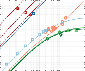
The proposed analytical model is compared against slip velocity of heavy particles, neutrally/marginally buoyant finite-size particles, and bubbles in homogeneous or quasi-homogeneous turbulence, as observed in laboratory experiments and direct numerical simulations listed in table 1. This allows us to validate the analysis across all practically interesting regions of the parameter space. For marginally buoyant finite-size particles, we deploy the form of the model derived in § 2.1 which neglects unsteady forces. The estimate of the fluid velocity at the particle location is discussed in the referenced works and extensively in other experimental and numerical studies (e.g. Horwitz & Mani Reference Horwitz and Mani2016; Berk & Coletti Reference Berk and Coletti2021). The specific approaches may lead to different instantaneous values, but the average of the observable is not expected to differ significantly. As shown in figure 8, the model is in quantitative agreement with the data for all regimes.
Table 1. Experimental and numerical studies reporting mean slip velocity of particles in homogeneous turbulence. Petersen, Baker & Coletti (Reference Petersen, Baker and Coletti2019), Bellani & Variano (Reference Bellani and Variano2012) and Clementi, Wedi & Coletti (Reference Clementi, Wedi and Coletti2024) used facing random jet arrays to generate homogeneous turbulence. Cisse, Homann & Bec (Reference Cisse, Homann and Bec2013) and Uhlmann & Chouippe (Reference Uhlmann and Chouippe2017) carried out particle-resolved simulations with an immersed boundary method in forced homogeneous isotropic turbulence, whereas Zhang et al. (Reference Zhang, Legendre and Zamansky2019) followed a point-particle approach. Ma et al. (Reference Ma, Lucas, Jakirlić and Fröhlich2020) considered the centre-plane region in a vertical channel flow simulated by the immersed boundary method.


Figure 8. Validation of model of particle slip velocity in homogeneous turbulence. The various cases from numerical and experimental data are summarised in table 1. Symbols represent reported values; lines of the same colour represent model predictions. For comparison with Ma et al. (Reference Ma, Lucas, Jakirlić and Fröhlich2020), only the SmFew case is considered as the model is limited to the one-way coupled regime.
4. Conclusions
Building on the framework of inertial filtering, we have developed an analytical model which captures the slip velocity magnitude of spherical non-tracer particles in homogeneous turbulence over the wide parameter space spanned by practically relevant applications, from light to heavy particles, from microscopic to finite size. The model takes two forms, derived for particles heavier and lighter than the fluid. The former retains only drag force and gravity effects, and is shown to be applicable also to marginally buoyant finite-size particles. The latter includes added mass and stress gradient forces and leverages the equilibrium Eulerian approximation, which in turn assumes small and weakly inertial particles.
The model is in quantitative agreement with experiments and direct numerical simulations. This has three important implications. First, it demonstrates that, for the purpose of predicting the magnitude of the mean slip velocity, the assumptions made are tenable. Those include: (i) Gaussian distribution of the slip velocity; (ii) small impact of history force and lift force, both neglected in the model; (iii) validity of the equilibrium Eulerian approximation for small light particles; (iv) negligible importance of unsteady forces for marginally buoyant particles; and (v) negligible difference between the flow scales experienced by particles and tracers. The prediction of higher-order observables, such as higher-order moments and two-point statistics, may require some of those simplifications to be relaxed. Second, the model is proven to yield valuable physical insight, capturing the specific influence of individual parameters on the slip velocity. Isolating the effect of each parameter is crucial for the predictive understanding of particle-laden turbulence, but is virtually impossible in physical experiments and typically beyond the reach of numerical simulations. Third, the ample validation warrants that the proposed model can make accurate predictions of the mean slip velocity purely from the governing parameters of the system. Therefore, we expect it to be useful for studies in which the slip velocity is an important parameter, e.g. to determine whether the dispersed phase is an accurate tracer and whether it is likely to back-react on the carrier fluid.
The model provides a theoretical underpinning for empirical observations which hitherto have only been qualitatively explained. For example, neutrally buoyant particles reportedly behave as tracers as long as  $d_p/\eta \lesssim 5$ (Qureshi et al. Reference Qureshi, Bourgoin, Baudet, Cartellier and Gagne2007; Volk et al. Reference Volk, Calzavarini, Lévêque and Pinton2011). Figure 8 shows how, for $Re_\lambda$ typical of experimental and numerical studies, this is precisely the size limit beyond which the mean slip velocity is not negligible, $\langle |u_s|\rangle >u_\eta$. In this regard, our results are complementary to those of Mathai et al. (Reference Mathai, Calzavarini, Brons, Sun and Lohse2016) who predict how particle accelerations depart from those of tracers as function of $St/Fr$. The present model also makes new predictions yet to be verified, specifically at high $Re_\lambda$.
Several extensions of the present model are possible. For example, the observed intermittency in the slip velocity distribution can be incorporated, which may be important to predict higher-order moments. The history force can be included if an integral expression is used, such as that proposed in Ling et al. (Reference Ling, Parmar and Balachandar2013) which however is only valid in a limited portion of the parameter space. Similarly, the lift force may be added using scaling dependencies with the governing parameters (Saffman Reference Saffman1956; Rubinow & Keller Reference Rubinow and Keller1961). Moreover, the model could be extended to non-homogeneous turbulence, using expressions for the temporal and velocity scale ratios valid for, e.g., turbulent boundary layers. Finally, the present framework may be applied to the important case of non-spherical particles (Voth & Soldati Reference Voth and Soldati2017), provided that the equation of motion is adequately parametrised.
Acknowledgements
The authors are grateful to T. Ma, M. Clementi and M. Wedi for providing their respective datasets.
Funding
The present work was supported in part by the US Army Research Office, Division of Earth Materials and Processes (grant W911NF-17-1-0366) and Division of Fluid Dynamics (grant W911NF-18-1-0354), and in part by the Swiss National Science Foundation (grant number 200021-207318).
Declaration of interests
The authors report no conflict of interest.
Appendix A
Using the relations provided at the end of § 2.1, the heavy-particle model given by (2.13) and (2.14) can be expressed in closed form as
 \begin{align} \frac{\langle |u_s|
\rangle}{u_\eta} &= {St} {Fr}^{{-}1} \mathrm{erf}\bigg\{
\bigg(\frac{1}{2}\frac{\langle u_s \rangle^2}{\langle
{u_s^\prime}^2\rangle}\bigg)^{1/2}\bigg\} \nonumber\\
&\quad +{St} \left( \frac{2}{\rm \pi}
\frac{Re_\lambda}{15^{1/2}} \right)^{1/2} \left(
\frac{Re_\lambda+32}{ 135^{1/2} (1-(0.1
Re_\lambda)^{{-}1/2})} + St\right)^{{-}1/2} \nonumber\\
&\quad \times \bigg( \frac{6 (1-(0.1
Re_\lambda)^{{-}1/2})}{10 (1+110 Re_\lambda^{{-}1})^{{-}1}}
+ St \bigg)^{{-}1/2} \exp\bigg\{-\frac{1}{2}\frac{\langle
u_s \rangle^2}{\langle {u_s^\prime}^2\rangle}\bigg\},
\end{align}
\begin{align} \frac{\langle |u_s|
\rangle}{u_\eta} &= {St} {Fr}^{{-}1} \mathrm{erf}\bigg\{
\bigg(\frac{1}{2}\frac{\langle u_s \rangle^2}{\langle
{u_s^\prime}^2\rangle}\bigg)^{1/2}\bigg\} \nonumber\\
&\quad +{St} \left( \frac{2}{\rm \pi}
\frac{Re_\lambda}{15^{1/2}} \right)^{1/2} \left(
\frac{Re_\lambda+32}{ 135^{1/2} (1-(0.1
Re_\lambda)^{{-}1/2})} + St\right)^{{-}1/2} \nonumber\\
&\quad \times \bigg( \frac{6 (1-(0.1
Re_\lambda)^{{-}1/2})}{10 (1+110 Re_\lambda^{{-}1})^{{-}1}}
+ St \bigg)^{{-}1/2} \exp\bigg\{-\frac{1}{2}\frac{\langle
u_s \rangle^2}{\langle {u_s^\prime}^2\rangle}\bigg\},
\end{align}with
 \begin{align} \frac{\langle u_s
\rangle^2}{\langle {u_s^\prime}^2\rangle} &=
\frac{15^{1/2}}{Re_\lambda} {Fr}^{{-}2}\left( \frac{Re_\lambda+32}{ 135^{1/2} (1-(0.1
Re_\lambda)^{{-}1/2})} + St\right) \nonumber\\ &\quad
\times\bigg(\frac{6 (1-(0.1
Re_\lambda)^{{-}1/2})}{10 (1+110 Re_\lambda^{{-}1})^{{-}1}}
+ St \bigg). \end{align}
\begin{align} \frac{\langle u_s
\rangle^2}{\langle {u_s^\prime}^2\rangle} &=
\frac{15^{1/2}}{Re_\lambda} {Fr}^{{-}2}\left( \frac{Re_\lambda+32}{ 135^{1/2} (1-(0.1
Re_\lambda)^{{-}1/2})} + St\right) \nonumber\\ &\quad
\times\bigg(\frac{6 (1-(0.1
Re_\lambda)^{{-}1/2})}{10 (1+110 Re_\lambda^{{-}1})^{{-}1}}
+ St \bigg). \end{align}
Appendix B
Using the relations provided at the end of 2.1, the light-particle model given by (2.26) and (2.27) can be expressed in closed form as
 \begin{align} \frac{\langle |u_s|
\rangle}{u_\eta} &= {St} {Fr}^{{-}1} \mathrm{erf}\bigg\{
\bigg(\frac{1}{2}\frac{\langle u_s \rangle^2}{\langle
{u_s^\prime}^2\rangle}\bigg)^{1/2}\bigg\} \nonumber\\
&\quad +{St} (\beta-1) \left( \frac{2}{\rm \pi}
\frac{Re_\lambda}{15^{1/2}} \right)^{1/2}
\left(\frac{Re_\lambda+32}{ 135^{1/2} (1-(0.1
Re_\lambda)^{{-}1/2})} + St\right)^{{-}1/2} \nonumber\\
&\quad \times\bigg(\frac{6 (1-(0.1
Re_\lambda)^{{-}1/2})}{10 (1+110 Re_\lambda^{{-}1})^{{-}1}}
+ St \bigg)^{{-}1/2} \exp\bigg\{-\frac{1}{2}\frac{\langle
u_s \rangle^2}{\langle {u_s^\prime}^2\rangle} \bigg\},
\end{align}
\begin{align} \frac{\langle |u_s|
\rangle}{u_\eta} &= {St} {Fr}^{{-}1} \mathrm{erf}\bigg\{
\bigg(\frac{1}{2}\frac{\langle u_s \rangle^2}{\langle
{u_s^\prime}^2\rangle}\bigg)^{1/2}\bigg\} \nonumber\\
&\quad +{St} (\beta-1) \left( \frac{2}{\rm \pi}
\frac{Re_\lambda}{15^{1/2}} \right)^{1/2}
\left(\frac{Re_\lambda+32}{ 135^{1/2} (1-(0.1
Re_\lambda)^{{-}1/2})} + St\right)^{{-}1/2} \nonumber\\
&\quad \times\bigg(\frac{6 (1-(0.1
Re_\lambda)^{{-}1/2})}{10 (1+110 Re_\lambda^{{-}1})^{{-}1}}
+ St \bigg)^{{-}1/2} \exp\bigg\{-\frac{1}{2}\frac{\langle
u_s \rangle^2}{\langle {u_s^\prime}^2\rangle} \bigg\},
\end{align}with
 \begin{align} \frac{\langle u_s
\rangle^2}{\langle {u_s^\prime}^2\rangle} &=
\frac{15^{1/2}}{Re_\lambda} {Fr}^{{-}2} (\beta-1)^{{-}2} \left( \frac{Re_\lambda+32}{
135^{1/2} (1-(0.1 Re_\lambda)^{{-}1/2})} + St\right)\nonumber\\ &\quad \times \bigg(
\frac{6 (1-(0.1 Re_\lambda)^{{-}1/2})}{10 (1+110
Re_\lambda^{{-}1})^{{-}1}} + St \bigg).
\end{align}
\begin{align} \frac{\langle u_s
\rangle^2}{\langle {u_s^\prime}^2\rangle} &=
\frac{15^{1/2}}{Re_\lambda} {Fr}^{{-}2} (\beta-1)^{{-}2} \left( \frac{Re_\lambda+32}{
135^{1/2} (1-(0.1 Re_\lambda)^{{-}1/2})} + St\right)\nonumber\\ &\quad \times \bigg(
\frac{6 (1-(0.1 Re_\lambda)^{{-}1/2})}{10 (1+110
Re_\lambda^{{-}1})^{{-}1}} + St \bigg).
\end{align}


 Open access