


1. Introduction
Emulsions, i.e. mixtures composed of two immiscible (totally or partially) liquids with similar densities, are extremely common in industrial applications, such as pharmaceuticals (Nielloud Reference Nielloud2000; Spernath & Aserin Reference Spernath and Aserin2006), food processing (McClements Reference McClements2015) and oil production (Kokal Reference Kokal2005; Mandal et al. Reference Mandal, Samanta, Bera and Ojha2010; Kilpatrick Reference Kilpatrick2012). Emulsions are also important in geophysical applications: as an example, when oil or industrial wastes spill into water streams (from rivers to oceans), the oil droplet distribution becomes fundamental for quantifying the environmental damage (Li & Garrett Reference Li and Garrett1998; French-McCay Reference French-McCay2004; Gopalan & Katz Reference Gopalan and Katz2010).
Indeed, when the inertia of the carrier fluid is stronger than the viscous forces (high Reynolds number) and the surface tension (high Weber number), the breakup of droplets due to the turbulent stresses produces broad distributions of droplet size. Droplet breakup, for a dilute emulsion in a homogeneous and isotropic turbulent flow, was investigated initially by Kolmogorov (Reference Kolmogorov1949) and Hinze (Reference Hinze1955), who derived an expression for the maximum size of droplets resisting breakup as a function of the flow characteristics and the fluid properties. This is usually referred to as the Kolmogorov–Hinze (KH) scale. Recent numerical investigations of droplets, bubbles and emulsions support the validity of the KH theory in both isotropic and homogeneous turbulence (Perlekar et al. Reference Perlekar, Benzi, Clercx, Nelson and Toschi2014; Mukherjee et al. Reference Mukherjee, Safdari, Shardt, Kenjereš and Van den Akker2019; Rivière et al. Reference Rivière, Mostert, Perrard and Deike2021a; Begemann et al. Reference Begemann, Trummler, Trautner, Hasslberger and Klein2022; Crialesi-Esposito et al. Reference Crialesi-Esposito, Rosti, Chibbaro and Brandt2022; Girotto et al. Reference Girotto, Benzi, Di Staso, Scagliarini, Schifano and Toschi2022), and in anisotropic flows (Rosti et al. Reference Rosti, Ge, Jain, Dodd and Brandt2020). Theoretical corrections were proposed recently to account for the scale-local nature of the process (Qi et al. Reference Qi, Tan, Corbitt, Urbanik, Salibindla and Ni2022; Crialesi-Esposito, Chibbaro & Brandt Reference Crialesi-Esposito, Chibbaro and Brandt2023a) and the fragmentation of droplets smaller than the KH scale (Vela-Martín & Avila Reference Vela-Martín and Avila2022).
At finite volume fraction of the dispersed phase, the presence of droplets modulates the underlying turbulence, affecting the flow statistics at both large (Yi, Toschi & Sun Reference Yi, Toschi and Sun2021; Wang et al. Reference Wang, Yi, Jiang and Sun2022) and small scales (Freund & Ferrante Reference Freund and Ferrante2019; Mukherjee et al. Reference Mukherjee, Safdari, Shardt, Kenjereš and Van den Akker2019; Vela-Martín & Avila Reference Vela-Martín and Avila2021; Crialesi-Esposito et al. Reference Crialesi-Esposito, Rosti, Chibbaro and Brandt2022). In turn, the modulation of the turbulent stresses by the dispersed phase influences the breakup of droplets, thus affecting the distribution of the droplet sizes.
Turbulence modulation in multiphase flows, i.e. the alterations of the flow with respect to single-phase turbulence, has been the object of several recent investigations. Not only are significant differences observed when density or viscosity contrasts between the phases are considered, but we also see a substantial modulation of the statistics at small scales for matching density and viscosity. In this case, the modulations are due solely to the presence of the interface and its surface tension.
Among the earliest works, Dodd & Ferrante (Reference Dodd and Ferrante2016) studied the dynamics of Taylor-scale-size droplets in decaying homogeneous isotropic turbulence (HIT). Examining the turbulent kinetic energy (TKE) budget, the authors showed that the total kinetic energy (encompassing the two phases) is compensating the surface area variations, e.g. TKE decreases when the interface increases, and vice versa. In the same work, the authors observed that discontinuities of velocity gradients may occur across the interface, an observation that led them to later use wavelet analysis to decompose the energy budget inside and outside the dispersed phase (Freund & Ferrante Reference Freund and Ferrante2019). This latest study showed that gradients caused by the interface enhance the production of small-scale energy in the dispersed phase. Similar conclusions were reached for sustained HIT by Mukherjee et al. (Reference Mukherjee, Safdari, Shardt, Kenjereš and Van den Akker2019) through vorticity analysis; these authors show that the interaction between surface tension and turbulence within the dispersed phase generates vortex compression and strain enhancement.
Vela-Martín & Avila (Reference Vela-Martín and Avila2021) demonstrate that the interface dynamics produces non-Gaussian statistics on the gradients within the dispersed phase, which hints at a significant modulation of the classic single-phase vortex stretching mechanism. Perlekar (Reference Perlekar2019) used the Cahn–Hilliard–Navier–Stokes equations to show that the energy transport mechanism is altered by the presence of the dispersed phase, also reporting a significant energy absorption at small scales due the chemical potential forcing. Crialesi-Esposito et al. (Reference Crialesi-Esposito, Rosti, Chibbaro and Brandt2022) observed that the presence of a dispersed phase modifies significantly the statistics at the small scales, producing large deviations from the average values of dissipation and vorticity. In the same work, the spectral scale-by-scale energy budget is used to show that energy is transported deep into the dissipative range by surface tension forces, ultimately forcing the viscous dissipation term to act at scales much smaller than those typical of single-phase turbulence for a similar large-scale forcing. Finally, Qi et al. (Reference Qi, Tan, Corbitt, Urbanik, Salibindla and Ni2022) observed that the droplet breakup is strongly affected by eddies smaller than the droplet size, suggesting that small-scale turbulence modulation is likely to be a major factor in the breakup dynamics.
A distinctive feature of the small-scale statistics in single-phase turbulent flows is the presence of intermittency (for a review of this topic, see, e.g. Sreenivasan & Antonia (Reference Sreenivasan and Antonia1997), Ishihara, Gotoh & Kaneda (Reference Ishihara, Gotoh and Kaneda2009), Kaneda & Morishita (Reference Kaneda and Morishita2012), and references therein). Early numerical simulations (Siggia Reference Siggia1981) and experiments (Meneveau & Sreenivasan Reference Meneveau and Sreenivasan1991) showed that the probability density function (PDF) of small-scale quantities, such as velocity gradients, vorticity and energy dissipation, are characterized by broad, non-Gaussian tails. This is in contrast with the large-scale statistics, which are generally Gaussian.
The development of broad tails in the PDFs of velocity increments at small scales breaks the scale invariance of the statistics, and causes the appearance of anomalous scaling exponents of the velocity structure functions (see e.g. Schumacher, Sreenivasan & Yakhot Reference Schumacher, Sreenivasan and Yakhot2007; Watanabe & Gotoh Reference Watanabe and Gotoh2007). While a first-principles derivation of the anomalous scaling exponents remains the Holy Grail of the theory of turbulence, several models have been proposed to parametrize the phenomenon of intermittency, notably in terms of the celebrated multifractal model (Benzi et al. Reference Benzi, Paladin, Parisi and Vulpiani1984; Frisch & Parisi Reference Frisch and Parisi1985; She & Leveque Reference She and Leveque1994).
In the light of the role played by intense velocity gradients in the process of droplets breaking, it is therefore interesting to understand how the interaction with the dispersed phase alters the intermittency in multiphase turbulent flows. Recent studies of bubble-laden flows showed that the introduction of bubbles into the flow strongly enhances intermittency in the dissipation range, while suppressing it at larger scales (Ma et al. Reference Ma, Ott, Frohlich and Bragg2021).
The purpose of the present work is to investigate how the presence of the dispersed phase alters the small-scale statistics in turbulent emulsions at large Reynolds and Weber numbers. In order to highlight the role of the interface separating the two phases, we focus on the the case of emulsions with matching density and viscosity between the two phases, and with moderate ( $10\,\%$) and high ( $50\,\%$) volume fractions. A case with large viscosity contrast is also considered for comparison.
To this aim, we examine the statistics of velocity increments between two points that are conditioned to be either in the same phase or in different phases, and find that the most important deviations from the statistics of single-phase flows, quantified by the PDFs of the velocity increments, are concentrated in regions around the interface, i.e. when the two points belong to different phases. We show that the contribution of the points located across the interface reduces the skewness of the PDFs as well as the amplitude of the third-order structure function. This is associated with a reduction of the flux of kinetic energy in the turbulent cascade. Finally, we discuss the effects of the droplets on the local scaling exponents of the high-order structure functions, which display a striking saturation at small scales.
The remainder of this paper is organized as follows. In § 2, we introduce the numerical method adopted for the simulations, while § 3 is devoted to the presentation of the results, and § 4 summarizes the main conclusions.
2. Numerical method and set-up of the simulations
We consider the velocity field  ${\boldsymbol u}({\boldsymbol x},t)$ obeying the Navier–Stokes equations
 \begin{equation} \rho ( \partial_t {\boldsymbol u} + {\boldsymbol u} \boldsymbol{\cdot} {\boldsymbol{\nabla} u} ) ={-} {\boldsymbol \nabla} p + {\boldsymbol \nabla} \boldsymbol{\cdot} [\mu ({\boldsymbol{\nabla} u} + {\boldsymbol{\nabla} u}^{\rm T} )] + {\boldsymbol f}^{\sigma} + {\boldsymbol f},\end{equation}
and the incompressibility condition  ${\boldsymbol \nabla } \boldsymbol {\cdot } {\boldsymbol u}=0$. In (2.1), $p$ is the pressure, $\rho$ is the density, and $\mu ({\boldsymbol x},t)$ is the local viscosity. The surface tension force is represented by the term ${\boldsymbol f}^{\sigma }=\sigma \xi \delta _S {\boldsymbol n}$, where $\sigma$ is the surface tension coefficient, $\xi$ is the local interface curvature, ${\boldsymbol n}$ is the surface normal unit vector, and $\delta _S$ represents a delta function that ensures that the surface force is applied at the interface only (Tryggvason, Scardovelli & Zaleski Reference Tryggvason, Scardovelli and Zaleski2011). The last term ${\boldsymbol f}$ is a constant-in-time body force that sustains turbulence by injecting energy at large scales. Here, we adopt the so-called ABC forcing (Mininni, Alexakis & Pouquet Reference Mininni, Alexakis and Pouquet2006), which reads
 \begin{equation} {\boldsymbol f}=\bigl(A\sin(\kappa_f z)+C\cos(\kappa_f y),B\sin(\kappa_f x)+A\cos(\kappa_f z), C\sin(\kappa_f y)+B\cos(\kappa_f x)\bigr). \end{equation}
The forcing scale is given by  $L_f = 2{\rm \pi} /\kappa _f$.
We solve (2.1) in a triply periodic, cubic domain of size  $L=2{\rm \pi}$, discretized on a staggered uniform Cartesian grid. Spatial derivatives are discretized with a second-order centred finite difference scheme and time integration performed by means of a second-order Adams–Bashforth scheme. A constant-coefficient Poisson equation is obtained using the pressure splitting method (Dodd & Ferrante Reference Dodd and Ferrante2014), which is solved using a fast Fourier transform direct solver. To reconstruct the interface, we use the algebraic volume of fluid method MTHINC, which solves the advection equation
 \begin{equation} \partial_t H + \boldsymbol{u}\,\boldsymbol{\nabla} H = 0,\end{equation}
for the colour function  $H$; this assumes the value $H=0$ in the carrier phase, and $H=1$ in the dispersed phase. The advection flux of $H$ in (2.3), the interface normal ${\boldsymbol n}$ and the curvature $\xi$ are computed according to Ii et al. (Reference Ii, Sugiyama, Takeuchi, Takagi, Matsumoto and Xiao2012). All the simulations have been performed with the open-source code FluTAS, described in Crialesi-Esposito et al. (Reference Crialesi-Esposito, Scapin, Demou, Rosti, Costa, Spiga and Brandt2023b), where further details on the numerical methods employed in this study can be found.
We consider four different cases, all using a fixed ABC forcing with  $A=B=C=1$ and $\kappa _f=2 {\rm \pi}/L_f=2$. The reference single-phase (SP) simulation has viscosity $\mu =0.006$ and unitary density $\rho =1$. For all multiphase (MP) simulations, the density ratio among the two phases is kept equal to $1$, and the surface tension is $\sigma =0.46$. We vary the volume fraction $\alpha =V_d/V$, defined as the ratio between the volume of the dispersed phase $V_d$ and the total volume $V=L^3$, and the viscosity ratio $\gamma =\mu _d/\mu _c$. Regarding the different volume fractions, we analyse the two cases with $\alpha =0.1$ (hereafter MP10) and $\alpha =0.5$ (hereafter MP50), while keeping $\gamma =1$ for both cases. Finally, we study the case $\alpha =0.1$ and viscosity ratio $\gamma =100$ (hereafter MPM), corresponding to the viscosity of the dispersed phase $\mu _d=0.6$.
All the simulations are performed at a resolution  $N=512$ which is sufficient to resolve all the scales (see Crialesi-Esposito et al. Reference Crialesi-Esposito, Rosti, Chibbaro and Brandt2022). The SP case is initialized using a perturbed ABC flow, which then evolves in time until a statistically stationary turbulent condition is reached. For the MP simulations, the dispersed phase is initially superposed to the pre-existing turbulent field as a single large droplet and let develop until statistically stationary conditions are reached. Statistics are accumulated over many large eddy turnover times $T=L_f/u_{rms}$ ( $136T$ for SP, $100T$ for MP10 and MP50, and
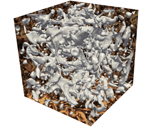
  $60T$ for MPM) once statistical stationary conditions have been reached. Figure 1 displays two examples of the droplet interface in stationary conditions for two of the configurations under consideration. The images exemplify the multiscale nature of turbulent emulsions, with a broad distribution of droplets of different sizes.

Figure 1. Rendering of the drop interface (corresponding to the value of the colour function  $H=0.5$) for the runs (a) MP10 and (b) MPM. The vorticity fields are shown on the box faces.
In table 1, we report the Taylor-scale Reynolds number  $Re_\lambda =u_{rms}\lambda /\nu$, the Taylor scale $\lambda =(15 u_{rms}\nu /\varepsilon )^{1/2}$ and the Kolmogorov scale $\eta = (\nu ^3/\varepsilon )^{1/4}$ for all the simulations. In the MP cases, these quantities are computed separately for the two phases. Here, and in the following, we identify the points belonging to the two phases according to the following criterion: points where the colour function assumes values $H({\boldsymbol x}) \le 0.1$ are assigned to the carrier phase, while points with $H({\boldsymbol x}) \ge 0.9$ correspond to the dispersed phase. For the MP cases, we also report the Weber number $We=\rho L_f u_{rms}^2/\sigma$ (defined in terms of the $u_{rms}$ of the carrier phase) and the normalized total interfacial area $A/L^2$. The KH scale $d_{KH}$ is computed as the scale (or equivalently the wavenumber $k$) at which the surface tension energy transfer function defined as
 \begin{equation} S_\sigma(k) =2\left\langle {\rm Re}\sum_{k<|\boldsymbol{k}|< k+1} \hat{\boldsymbol f}^\sigma ({\boldsymbol k},t) \boldsymbol{\cdot} \hat{\boldsymbol u}^*({\boldsymbol k},t) \right\rangle_t,\end{equation}
is null. Here,  $\hat {\cdot }$ is the Fourier transform operator, and $\langle \cdot \rangle _t$ denotes the time average. The estimation of the KH scale through $S_\sigma (k)$ is preferred here to its classic expression (Hinze Reference Hinze1955) as it can be computed through exact quantities, avoiding the need for arbitrary constants, such as the critical Weber number (Crialesi-Esposito et al. Reference Crialesi-Esposito, Chibbaro and Brandt2023a).
Table 1. The table reports the values of the Taylor–Reynolds number  $Re_\lambda ^{c,d}$, the Taylor scale $\lambda ^{c,d}$ and the Kolmogorov scale $\eta ^{c,d}$ separately for the carrier (superscript c) and dispersed (superscript d) phases. For the MP cases, we also report the Weber number $We$, the KH scale $d_{KH}$, and the normalized total interfacial area $A/L^2$. The values of $\lambda$ and $d_{KH}$ are non-dimensionalized with the forcing scale $L_f={\rm \pi}$.

3. Statistics of the multiphase flow
In turbulent MP flows, part of the kinetic energy of the carrier phase is absorbed at large scales by the deformation and breakup of the interface of the dispersed phase, while the coalescence of small droplets, their surface oscillations and relaxation from high local curvature re-inject energy in the carrier phase at small scales. The consequences of this complex exchange of energy between the two phases are evident in the kinetic energy spectrum shown in figure 2. Comparing the spectra of an MP flow with that of an SP flow sustained by the same forcing, we observe a suppression of energy at low wavenumbers (i.e. large scales with  $\kappa /\kappa _f\lesssim 10$) and an enhancement at high wavenumbers ( $\kappa /\kappa _f\gtrsim 10$). This effect increases with the volume fraction $\alpha$ of the dispersed phase (Mukherjee et al. Reference Mukherjee, Safdari, Shardt, Kenjereš and Van den Akker2019; Crialesi-Esposito et al. Reference Crialesi-Esposito, Rosti, Chibbaro and Brandt2022).

Figure 2. Kinetic energy spectra of SP flow (black solid line), and MP flows at  $\alpha =0.1$ (red dashed line) and $\alpha =0.5$ (blue dash-dotted line). Vertical solid lines represent the KH scales reported in table 1, with corresponding colouring.
The interaction between the fluid–fluid interface and turbulence produces a polydisperse droplet size distribution, which is shown in figure 3 in terms of the PDF of the droplet diameter together with the scaling laws proposed in the literature. We recall that the KH theory predicts that the breakup of droplets larger than the KH scale  $d_{KH}$ follows a cascade-like process, described by Garrett, Li & Farmer (Reference Garrett, Li and Farmer2000) with a $d^{-10/3}$ power law, and observed in numerical (Deike, Melville & Popinet Reference Deike, Melville and Popinet2016; Mukherjee et al. Reference Mukherjee, Safdari, Shardt, Kenjereš and Van den Akker2019; Crialesi-Esposito et al. Reference Crialesi-Esposito, Rosti, Chibbaro and Brandt2022) and experimental (Garrett et al. Reference Garrett, Li and Farmer2000; Deane & Stokes Reference Deane and Stokes2002) studies. For droplets smaller than $d_{KH}$, the PDF displays $d^{-3/2}$ power-law behaviour, in agreement with previous studies (Rivière et al. Reference Rivière, Mostert, Perrard and Deike2021a,Reference Rivière, Ruth, Mostert, Deike and Perrardb; Crialesi-Esposito et al. Reference Crialesi-Esposito, Rosti, Chibbaro and Brandt2022; Deane & Stokes Reference Deane and Stokes2002).

Figure 3. PDFs of droplet diameters. The dashed black line represents the  $d^{-3/2}$ law for droplets smaller than the KH scale (Deane & Stokes Reference Deane and Stokes2002), and the dash-dotted black line represents the $d^{-10/3}$ law describing a cascade-like process at larger scales (Garrett et al. Reference Garrett, Li and Farmer2000).
Further comparing the PDFs of the MP10 and MP50 cases, we observe that the major effect of increasing the volume fraction is to increase the number of large drops, while the statistics of the small drops remains almost unchanged. As a result of the different form of the PDFs, the total interface area (reported in table 1) does not follows the dimensional scaling  $A/L^2 \sim (V_d/V)^{2/3}$.
Because of the injection of energy at small scales by the droplet dynamics (at  $\kappa /\kappa _f \gtrsim 10$; see figure 2), we expect higher intermittency of the velocity fluctuations in the MP flow than in the SP flow at fixed amplitude of the external forcing. In order to quantify this effect, we compute the PDFs of the longitudinal velocity increments $\delta _{\ell } u=({\boldsymbol u}({\boldsymbol x}_2)-{\boldsymbol u}({\boldsymbol x}_1)) \boldsymbol {\cdot } ({\boldsymbol x}_2-{\boldsymbol x}_1)/\ell$ at distance $\ell =|{\boldsymbol x}_2-{\boldsymbol x}_1|$. The comparison of the PDFs at two scales within the inertial range, shown in figure 4, confirms that the velocity increments have larger fluctuations in the case of MP flows, in particular at smaller values of $\ell$. This effect increases with the concentration $\alpha$ of the dispersed phase. We also observe that in the case $\gamma =100$ (i.e. when the dispersed phase is much more viscous than the carrier phase), the effect of the droplets on the velocity increments vanishes due to the damping of fluctuations in the dispersed phase, and we recover the statistics of the SP flow.

Figure 4. PDF of velocity increments at distance (a)  $\ell = 0.03L_f$ and (b) $\ell = 0.12L_f$, normalized by the standard deviation of the SP case. The SP Kolmogorov scale is $\ell \approx 0.008L_f$. The dotted black line represents a standard Gaussian distribution.
Note that the PDFs shown in figure 4 are computed over the full simulation domain, i.e. the velocity increments are computed among points  ${\boldsymbol x}_{1,2}$ that belong to both phases unconditionally. To understand the role of the interface in the turbulent statistics, we introduce three different PDFs of the velocity increments, depending in which phase the two points ${\boldsymbol x}_1$ and ${\boldsymbol x}_2$ are immersed. We denote by $P_{cc}$, $P_{dd}$ and $P_{cd}$ the PDFs relative to points belonging only to the carrier phase $c$, only to the dilute phase $d$, and to points belonging to different phases, respectively. The velocity increments in which one of the two points lies on the interface ( $0.1< H({\boldsymbol x})<0.9$) are not considered in the statistics.
Figures 5(a) and 5(b) show the conditional PDF (normalized with the corresponding variance of the SP case) pertaining to the simulation with volume fraction  $\alpha =0.1$ at two scales $\ell$ within the inertial range. First, we note that the PDF of the carrier phase is similar to that of the SP case (and this is the case also for the variance). In the dispersed phase, on the contrary, velocity increments develop a relatively large negative tail at small separations. Remarkably, $P_{cd}$ develops the largest positive tail at small scales (figure 5a), a clear indication of the role of the interface for small-scale intermittency in MP flows.

Figure 5. PDFs of velocity increments conditioned to the phases on which the two velocities are measured:  $cc$ (both points in the carrier phase, red line), $dd$ (both points in the dispersed phase, orange line), $cd$ (one point in each phase, blue line). (a,b) Simulation MP10 with $\alpha =0.1$ and $\gamma =1$. (c,d) Simulation MP50 with $\alpha =0.5$ and $\gamma =1$. (e,f) Simulation MPM with $\alpha =0.1$ and $\gamma =100$. Black line indicates PDF of velocity increments for the SP simulation. Dashed black line indicates Gaussian distribution. All the PDFs are rescaled with the variance of the SP case.
Similar observations can be made for the simulation MP50 shown in figures 5(c,d). We remark that in this case, the two phases are equivalent ( $\alpha =0.5$ and $\gamma =1$) and therefore $P_{dd}=P_{cc}$, which also confirms the validity of our statistical sample. Figure 5 shows that the leading contribution to the increased deviation from Gaussian statistics at small scales comes from velocity increments across the interface, $P_{cd}$. Note that although the shapes of $P_{cd}$ are similar for MP10 and MP50, their contributions to the overall flow statistics are different because of the different statistical weight (i.e. the different extension of the total interface).
Finally, the scenario is substantially different for the MPM case in which  $\gamma =100$ (figures 5e,f). In this case, the flow inside the dispersed phase is strongly suppressed by the large viscosity, as shown by the small value of the phase Reynolds number $Re_\lambda ^d = 5$. Therefore, the velocity increments in the dispersed phase $P_{dd}$ are almost vanishing, and the PDF displays a neat peak around $\delta _\ell u \approx 0$. Similarly, the velocity increments across the interface are reduced because of the contribution of the point inside the droplet. This leads to behaviour similar to that of the SP flow for the velocity increments in the carrier phase $P_{cc}$.
A remarkable feature shown in figure 5 is that the skewness of  $P_{cd}$ at small scales is opposite (i.e. positive) to that of $P_{cc}$. We quantify this effect by computing the skewness $Sk(\ell )=S_3(\ell )/S_2(\ell )^{3/2}$, defined in terms of the structure functions $S_p(\ell )=\langle (\delta _{\ell } u)^p \rangle$, where the average can be unconditioned or conditioned to two points belonging either to the carrier phase $S_p^{cc}(\ell )$ or to the dispersed phase $S_p^{dd}(\ell )$, or points located on different sides of the interface, $S_p^{dc}(\ell )$. As in the case of the PDFs, we exclude from the statistics the points that lie on the interface. Consistently, $S_p^{cd}(\ell )$ is computed only for distance $\ell > 3\,{\rm \Delta} x$.
The values of the skewness are shown in figures 6(a,c,e). The skewness of the SP case is always negative, as well as that of the MP cases in which the statistics is either unconditioned or conditioned to a single phase ( $Sk_{cc}$ and $Sk_{dd}$). At small scales, $Sk$ becomes almost flat because of the smooth velocity increments in the viscous range $\delta u_\ell \sim \ell$.

Figure 6. (a,c,e) Skewness  $Sk(\ell )$, and (b,d,f) third-order structure function $S_3(\ell )$. Data show simulation results for (a,b) $\alpha =0.1$ and $\gamma =1$, (c,d) $\alpha =0.5$ and $\gamma =1$, and (e,f) $\alpha =0.1$ and $\gamma =100$. Data are averaged on the whole domain for the SP case in black, and for the MP cases in violet. Data for $cc$,
$cc$,  $dd$ and $cd$ show the conditional averages.
Different behaviour is observed for the skewness  $Sk_{cd}$ of velocity increments across the interface, which is always larger than $Sk_{cc}$ and $Sk_{dd}$. Notably, for MP50 (figure 6c), $Sk_{cd}$ reaches positive values at scales within the inertial range.
In the case of SP turbulent flows, the negative sign of the skewness is a manifestation of the energy cascade towards small scales. Under the assumption of local statistical stationarity and homogeneity, the Kolmogorov  $4/5$ law gives $S_3(\ell ) = -(4/5) \varepsilon \ell$ in the inertial range, where the viscous energy dissipation rate $\varepsilon$ is equal to the flux of the turbulent cascade (Frisch Reference Frisch1995). Therefore, the amplitude of $S_3(\ell )$ is proportional to the energy flux, and the negative skewness $Sk({\ell })$ indicates the direction of the energy transfer. Therefore, the amplitude of $S_3(\ell )$ is proportional to the energy flux, and a negative skewness indicates the direction of the energy transfer to small scales.
In MP flows, because of the opposite sign of the skewness of  $P_{cd}$ with respect to $P_{cc}$, we expect that the presence of the interface reduces the energy flux associated with the turbulent cascade. This can be quantified by looking at the third-order velocity structure function $S_3(\ell )$ in figures 6(b,d,f).
The data in figure 6 reveal that the third-order structure function of the MP turbulent flows is qualitatively similar to the SP flow when averaged over the whole domain, yet with a smaller amplitude. This is due to the fact that part of the turbulence energy is used to break the interface, and the direct transfer of energy to small scales is reduced (Crialesi-Esposito et al. Reference Crialesi-Esposito, Rosti, Chibbaro and Brandt2022). If we consider the same quantity averaged over one of the two phases only –  $S_3^{cc}(\ell )$ and $S_3^{dd}(\ell )$, which are equivalent in a binary flow – then the magnitude of the flux increases and approaches the SP limit, indicating that the turbulent cascade is not significantly affected when considering only flow structures living in one of the two phases. On the contrary, the flux across two points belonging to different phases is strongly suppressed: the associated $S_3^{dc}(\ell )$ is closer to zero and even changes sign at intermediate scales for $\alpha =0.5$ (consistently with what is suggested in figure 5). The physical interpretation is that the interface ‘decouples’ the velocity fields in the two phases, which become less correlated and therefore have a reduced energy flux, signalled by the reduction of $S_3(\ell )$. The precise behaviour of $S_3^{dc}(\ell )$ depends on the value of $\alpha$, as shown by the comparison with the case $\alpha =0.1$ (see figures 6a,c,e). Nevertheless, the reduction of the energy flux at intermediate scales is a general feature, independent of $\alpha$.
For high viscosity of the dispersed phase, case MPM displayed in figures 6(e,f), the energy fluctuations in the dispersed phase are substantially damped, as shown by  $S_3^{dd}$, which supports the discussion of the results reported in figure 4. As a consequence, the flow in the carrier phase is only slightly affected by the presence of the dispersed phase, with negligible effects when compared to the SP case. Finally, it is worth noting that at very large scale, only very few droplets of comparable size are formed, hence only limited data are available for the statistics.
The effects of the presence of a dispersed phase on the statistics of the velocity fluctuations affects also the scaling behaviour of the structure functions of the absolute values of the longitudinal velocity increments defined as  $S^a_p(\ell ) = \langle |\delta _{\ell } u|^p \rangle$. It is well known that in SP flows, the structure functions display a power-law behaviour $S^a_p(\ell ) \sim \ell ^{\zeta _p}$ at scales $\ell$ in the inertial range (Frisch Reference Frisch1995). In this context, intermittency manifests in the nonlinear behaviour of the scaling exponents: $\zeta _p \neq p/3$. In the MP flows, because of the different physical processes that occur at scales larger and smaller than the KH scale (dominated by breakup and coalescence, respectively), we expect to observe a more complex scaling behaviour. To address this issue, we compute the local scaling exponents defined as the logarithmic derivatives of the structure functions, $\zeta _p(\ell ) = {\text {d} \log (S^a_p(\ell ))}/{\text {d} \log (\ell )}$, and here applied to MP flows for the first time.
The local scaling exponents  $\zeta _p(\ell )$ (computed over the whole domain) are displayed for $p \le 8$ in figure 7, where they are divided by the reference scaling exponent $\zeta _3(\ell )$ of the third-order structure function. We recall that plotting the ratio $\zeta _p(\ell ) / \zeta _3(\ell )$ is equivalent to the extended self-similarity method (Benzi et al. Reference Benzi, Ciliberto, Tripiccione, Baudet, Massaioli and Succi1993), which has been shown to improve the scaling range at moderate Reynolds numbers. In the SP case (figure 7a), we find that the ratios $\zeta _p(\ell )/\zeta _3(\ell )$ are almost constant in the inertial range $0.09\le \ell /L_f \le 0.32$. In the MP flows, the values of the exponents are a little smaller but comparable to that of the SP case only at large scales; we observe a dramatic decrease of the scaling exponents at scales $\ell$ smaller than the KH scale $L_{KH} \approx 0.14 L_f$ for the case MP10 (figure 7b) and $L_{KH} \approx 0.19 L_f$ for the case MP50 (figure 7c) (see vertical lines in the figure). In particular, we observe a striking saturation of the scaling exponents of the high-order structure function with $p \ge 5$ at scales $\ell \approx 0.02 L_f$ for the MP50 case and $\ell \approx 0.04 L_f$ for the MP10 case. The saturation of the scaling exponents of the high-order structure functions reveals the presence of strong velocity differences across the interface between the two phases.

Figure 7. Local scaling exponents  $\zeta _p$ of the structure functions, for (a) SP, (b) MP10 at $\alpha =0.1$, (c) MP50 at $\alpha =0.5$, and (d) MPM at $\gamma =100$. The structure functions are computed by averaging over the whole domain. In each plot, the exponents of different order $p$ assume increasing values (the value of $p$ is reported above each curve). Curves for $p=3$ are omitted. Vertical black dashed lines represent the KH scale, computed as in Crialesi-Esposito et al. (Reference Crialesi-Esposito, Chibbaro and Brandt2023a).
Note also that the saturation of the exponents is not observed when the dispersed phase presents higher viscosity, case MPM in figure 7(d). This is consistent with the previous observations in figure 5(e), which shows that velocity gradients across the interface are significantly reduced.
4. Conclusions
We have discussed intermittency and scaling exponents obtained from direct numerical simulations of turbulent emulsions at moderate ( $10\,\%$) and high ( $50\,\%$) volume fractions, and two different values of the viscosity contrast. As observed in previous works (Perlekar Reference Perlekar2019; Pandey, Ramadugu & Perlekar Reference Pandey, Ramadugu and Perlekar2020; Crialesi-Esposito et al. Reference Crialesi-Esposito, Rosti, Chibbaro and Brandt2022), the presence of a deformable interface increases the intermittency in the flow and the energy content at small scales, when the surface tension offers an alternative path for energy transport across scales.
By investigating the statistics of the velocity increments conditioned to points belonging to a single phase or to different phases, we demonstrate that the increased intermittency is due mostly to the presence of strong velocity differences across the interface between the carrier and the dispersed phase.
We also show that the presence of the dispersed phase causes a decrease of the negative skewness of the PDF of the longitudinal velocity increments. This is associated with a reduction of the flux of the kinetic energy from the forcing scale to the viscous scales, which is due to the absorption and dissipation of part of the kinetic energy of the turbulent flow by the deformation and breakup of drops of the dispersed phase. This reduction increases with the volume fraction so that the flux related to points lying on either side of the interfaces eventually gives a positive contribution to the distribution skewness at the highest volume fraction considered here.
Finally, to understand the local properties of turbulence, we have analysed the longitudinal structure functions at higher orders. Interestingly, at scales larger than the Kolmogorov–Hinze (KH) scale, the exponents are only slightly smaller than in the single-phase (SP) flow, which implies increased intermittency, yet a similar anomalous scaling. More importantly, we report a neat saturation of the exponents for structure functions higher than 3 at small scales. This saturation seems to occur at scales smaller than the KH length, but further analysis at different  $We$ should be performed to confirm this hypothesis. These effects disappear for the simulation with viscosity ratio $\gamma =100$. In this case, the high viscosity of the dispersed phase reduces the deformability of the interface and globally suppresses velocity fluctuations at small scales.
These observations may prove fundamental for understanding small-scale dynamics in MP flows and for their future sub-grid modelling. Indeed, our results indicate that a correct model would need to account for the reduction of the energy fluxes near an interface. Moreover, we have shown that the turbulence statistics approach those of the SP flow when the droplets consist of a highly viscous fluid. This suggests that despite several global measures seeming to indicate a similar dynamics (Olivieri, Cannon & Rosti Reference Olivieri, Cannon and Rosti2022; Yousefi Reference Yousefi2022), the turbulence modulation is significantly different in the case of rigid particles and deformable inclusions.
Acknowledgements
M.C.-E., G.B. and S.M. acknowledge support from the Departments of Excellence grant (MIUR) and INFN22-FieldTurb. The authors acknowledge computer time provided by the National Infrastructure for High Performance Computing and Data Storage in Norway (Sigma2, project no. NN9561K) and by SNIC (Swedish National Infrastructure for Computing).
Funding
L.B. acknowledges support from the Swedish Research Council via the multidisciplinary research environment INTERFACE, Hybrid multiscale modelling of transport phenomena for energy efficient processes, grant no. 2016-06119.
Declaration of interests
The authors report no conflict of interest.
Data availability statement
Data are available from the corresponding author upon reasonable request.


