


Introduction
Only a very small number of the thousands of known natural minerals constitute most magmatic rocks. Olivine, pyroxene, amphibole, mica, feldspar, feldspathoids, Fe–Ti oxides (magnetite and ilmenite), and quartz are typically the major constituents in magmatic rocks. Aprart from quartz these are all solid solutions. It is a simple task to identify these minerals in hand sample with the aid of a hand lens in the field or in thin section using a polarising microscope in the laboratory. X-ray diffraction and scanning electron microscopy studies are other common options for mineral identification. Electron microprobe analysis (EPMA) is one of the most widely used instruments for compositional analysis of minerals (Best, Reference Best2003), and these data are commonly reported in weight percentages of the oxides of the measured elements. These data require calculation of cationic formula and end-member components of each analysed mineral. Such calculations can be easily performed using published mineral formulae calculation programs that are mainly free Excel-based applications. Most of these programs are mineral-specific formulae calculators with, or without, thermobarometry tools, for example: amphibole (Yavuz, Reference Yavuz1996, Reference Yavuz2007; Locock, Reference Locock2014; Li et al., Reference Li, Zhang, Behrens and Holtz2020a); mica (Yavuz and Öztaş, Reference Yavuz and Öztaş1997; Yavuz, Reference Yavuz2001; Li et al., Reference Li, Zhang, Behrens and Holtz2020b); pyroxene (Yavuz, Reference Yavuz2013); garnet (Yavuz and Yildirim, Reference Yavuz and Yildirim2020); tourmaline (Yavuz, Reference Yavuz1997); and magnetite–ilmenite (Lepage, Reference Lepage2003; Hora et al., Reference Hora, Kronz, Möller-McNett and Wörner2013; Yavuz, Reference Yavuz2021). A few general mineral formulae calculation programs also included in the literature are: Afifi and Essene (Reference Afifi and Essene1988); Rock and Caroll (Reference Rock and Caroll1990); Griffin et al. (Reference Griffin, Muhling, Carroll and Rock1991); De Bjerg et al. (Reference De Bjerg, Mogessie and Bjerg1992, Reference De Bjerg, Mogessie and Bjerg1995); Brandelik (Reference Brandelik2009) etc. In addition, there are many unpublished mineral formula calculators that can be downloaded from web-pages or obtained from their developers. Structural formulae and end-member calculations from mineral compositional analyses are routine intermediate tasks for classification purposes before further petrological calculations can be made (e.g. geothermobarometry, fugacity, magmatic water content, phase equilibria etc.). For the case of geothermobarometry, the programs listed above either include no computations or some only for a specific mineral, implying they are not comprehensive thermobarometry tools.
MagMin_PT is designed mainly as a comprehensive geothermobarometry tool for igneous systems as shown in Fig. 1, which can also be used as a classical mineral classification calculator. Therefore, MagMin_PT includes various classification diagrams and P–T plots for the most common igneous rock-forming minerals (e.g. olivine, pyroxene, amphibole, biotite, feldspar, magnetite, ilmenite, apatite and zircon) with minerals and groups defined according to the International Mineralogical Association (IMA).
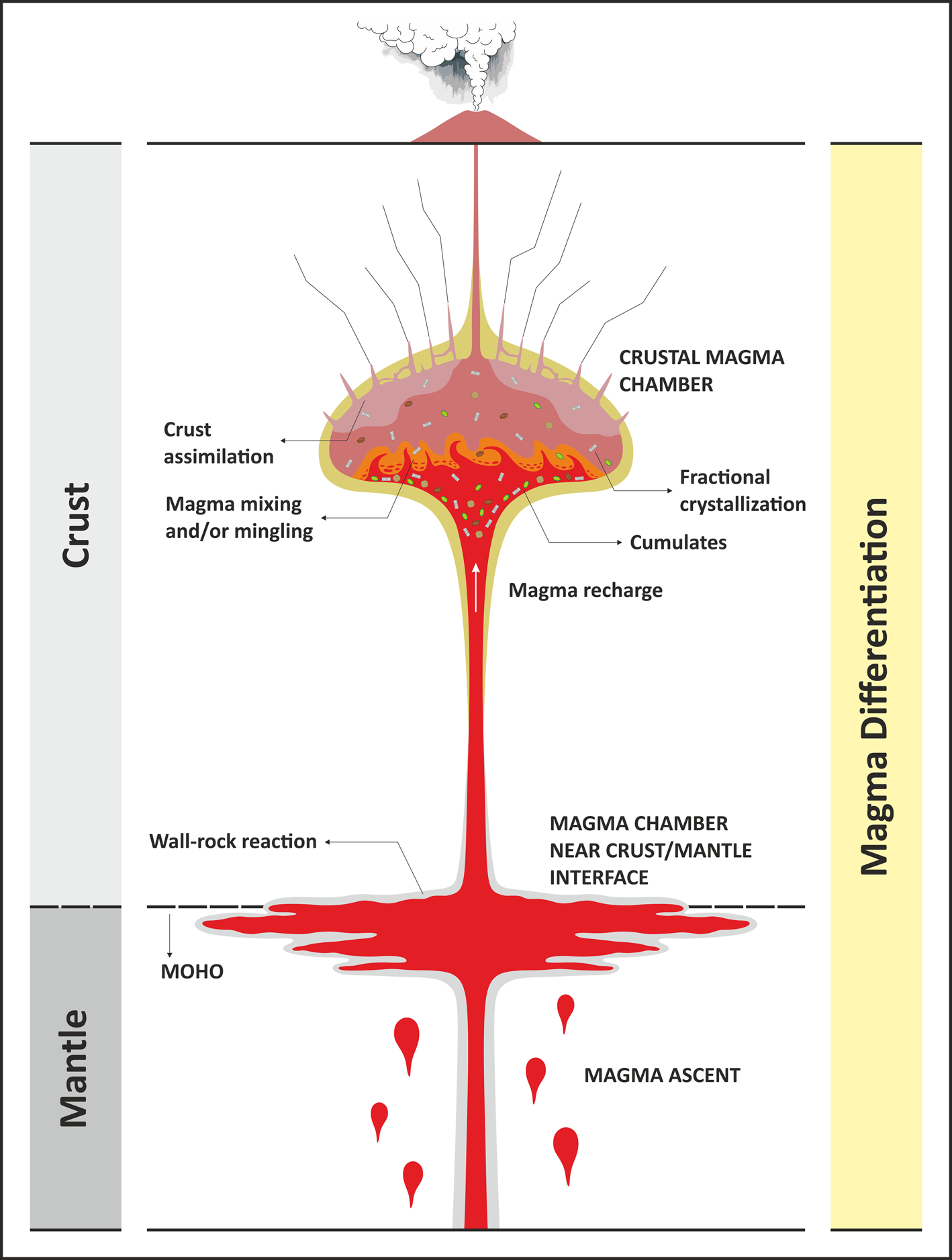
Fig. 1. A conceptual diagram showing the ascent of magma and main differentiation processes in a crustal-magma chamber such as fractional crystallisation, assimilation, and magma mixing.
Principles of mineral formula calculation
The recasting of compositional data into a mineral formula is a series of mathematical functions based on the atomic weight, charge of cation, etc. of the elements analysed (see Brandelik, Reference Brandelik2009) and which depends on the structure of the minerals, and relationships between charge neutrality and crystal chemistry (e.g. 4 oxygens for olivines, 6 oxygens for pyroxenes etc.). Following the scheme of Deer et al. (Reference Deer, Howie and Zussman1992), the main steps for mineral formula calculation are given in Table 1, using olivine as an example.
Table 1. Structural formula calculation of an olivine* composition obtained by electron microprobe analysis.
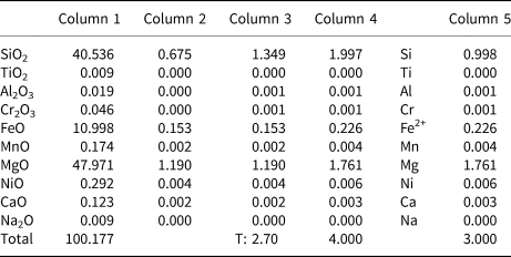
Calculation notes: Column 1: The composition of the olivine as weight percentages of the oxides (wt.%), derived from EPMA.
Column 2: Molecular proportions of the oxides, derived by dividing each column (1) entry by the molecular weight (Wieser and Berglund, Reference Wieser and Berglund2009) of the oxide concerned.
Column 3: Atomic proportion of oxygen from each molecule, derived from column (2) by multiplying by the number of oxygen atoms in the oxide concerned. At the foot of column (3) is its total (T).
Column 4: No. of anions on the basis of 4 oxygens (e.g. olivine formula based on 4 oxygen atoms), done by multiplying all of the oxides in column 3 by 4/T. For this case the multiplier is 4/2.70 = 1.48.
Column 5: No. of ions in the formula, the number of cations associated with the oxygens in column (4). Thus, for SiO2 and TiO2 the column (4) entry is divided by 2, for Al2O3 the column (4) entry is multiplied by 2/3. For divalent ions (FeO, MgO, MnO, NiO, CaO) the column (5) value is the same that of column (4). If there are monovalent ions (e.g. K2O, Na2O) in the analysis, they are doubled in column (5), which is not case in the olivine formula here.
* Olivine data from Asan et al. (Reference Asan, Kurt, Gündüz, Gençoğlu Korkmaz and Morgan2021)
This procedure can be easily used for anhydrous minerals (olivine, pyroxene, feldspar etc.) whose cation-sites are full and the total weight percentage of major oxides are ~100%. However, hydrous minerals such as amphibole and biotite have a more complex mineral chemistry that cannot be fully determined by routine instrumental techniques. The main problem is that electron microprobe analysis cannot directly determine the volatile contents of hydrous minerals and does not differentiate between the valence states of iron (Fe2+, Fe3+), thus requiring additional computations. Such computations can be relatively easily made for anhydrous minerals if it is assumed that they have full-cation sites and perfect charge balance, however this is not always straightforward for hydrous minerals. Therefore, many classification schemes and methods have been proposed for hydrous minerals over time, depending on the development of analytical techniques and computer science. In the program MagMin_PT, users can find diverse mineral formula calculation methods based on traditional computations, and to some extent machine learning methods which have become popular recently in geothermobarometry (Li et al., Reference Li, Zhang, Behrens and Holtz2020a, Reference Li, Zhang, Behrens and Holtz2020b; Petrelli et al., Reference Petrelli, Caricchi and Perugini2020; Higgins et al., Reference Higgins, Sheldrake and Caricchi2022).
Tests for liquid equilibria in P–T calculations
The application of any geothermobarometry is inevitably related to chemical equilibrium between phases (e.g. liquid–mineral or mineral–mineral). In MagMin_PT, various P–T calculations are based on the application of mineral–liquid thermobarometry, requiring tests for equilibrium before calculations. Users can test equilibrium between mineral–liquid pairs in different ways: (1) petrographic observations; (2) calculation of mineral–liquid partition coefficients; and (3) comparing predicted and calculated mineral components (see Putirka, Reference Putirka, Putirka and Tepley2008 for details).
Textural features observed using polarised-light microscopy or more advanced imaging methods (back-scattered electron (BSE) or cathodoluminescence (CL) petrography) can be first employed to evaluate equilibrium between selected mineral–liquid pairs. The predominant euhedral habit of minerals is generally considered to be evidence of equilibrium with the liquid in which they occur. In contrast, disequilibrium textures in minerals suggest that this condition is not met. Such textural features are diverse, especially in volcanic rocks and include: crystal zoning; resorption and dissolution surfaces; reaction rims; pseudomorphs; overgrowths on existing minerals; crystal clots etc. (Ginibre et al., Reference Ginibre, Wörner and Kronz2007; Streck, Reference Streck, Putirka and Tepley2008). Therefore, these textures are the best indicators that minerals were out of equilibrium and that they reacted with the enclosing liquid.
Mineral–liquid thermobarometers are imported from Putirka's equations and are based mostly on iterative equations. Calculation of mineral–liquid partition coefficients is another test for equilibrium that can be automatically made in MagMin_PT. Composition of a glass or whole rock, or some calculated composition can be used as the liquid. The partitioning of Fe–Mg between mineral–liquid pairs (e.g. the Fe–Mg exchange coefficient) is used for mafic minerals (olivine, orthopyroxene, clinopyroxene and amphibole) in MagMin_PT and is based on the following general equations, originally suggested for olivine by Roeder and Emslie (Reference Roeder and Emslie1970):


The acceptable partition coefficient (KD) range for each mineral to be equilibrium with the liquid will be given in the next section.
Comparing predicted and calculated mineral components is a test for equilibrium. The test is to compare predicted and observed values for the clinopyroxene components, producing a bivariate plot. This is based on the idea that predicted and observed values are close to each other under equilibrium conditions. This method is only applicable to clinopyroxene in MagMin_PT.
Program description
MagMin_PT is a Microsoft® Excel© workbook that is specifically designed for the needs and demands of researchers working with mineral compositional data and the geothermobarometry of magmatic rocks. It is divided into eleven Excel sheets: ‘Instructions’, ‘Data Input’, ‘Olivine’, ‘Pyroxene’, ‘Amphibole’, ‘Biotite’, ‘Feldspar’, ‘Magnetite-Ilmenite’, ‘Apatite’, ‘Zircon’ and ‘Conversions’. These sheets are summarised in the following section, based on their principal role in the program.
Instructions
Instructions are given on this sheet in the program. Note: if users encounter an Excel-Circular Reference problem, they need to go to File > Options > Formulas, and select the ‘Enable iterative calculation’ check box in the Calculation options section. After clicking on the check boxes in the ‘Data Input’ spreadsheet, the output of formula proportions in atoms per formula unit (apfu) and thermobarometry results can take a few seconds due to iterative equations.
Data Input
‘Data Input’ contains access to the spreadsheets for user data (i.e. major oxides-wt.% of mineral and glass/whole-rock compositions). First, to enable data entry the check boxes on the ‘Data Input’ spreadsheet must be clicked in the order: (1) select ‘Data input’; (2) select the appropriate ‘Mineral’ and enter compositions in the appropriate panel on the right; (3) select ‘Calculation’ to enable the calculation of cation formula and P–T results – presented in the subsequent sheets (Fig. 2). In the majority of the ‘Data Input’ sheets, the upper right panel is for mineral compositions, the lower right panel is for ‘glass’ or ‘whole-rock compositions’ – the latter should be used if users want to make P–T calculations based on mineral–liquid geothermobarometry.
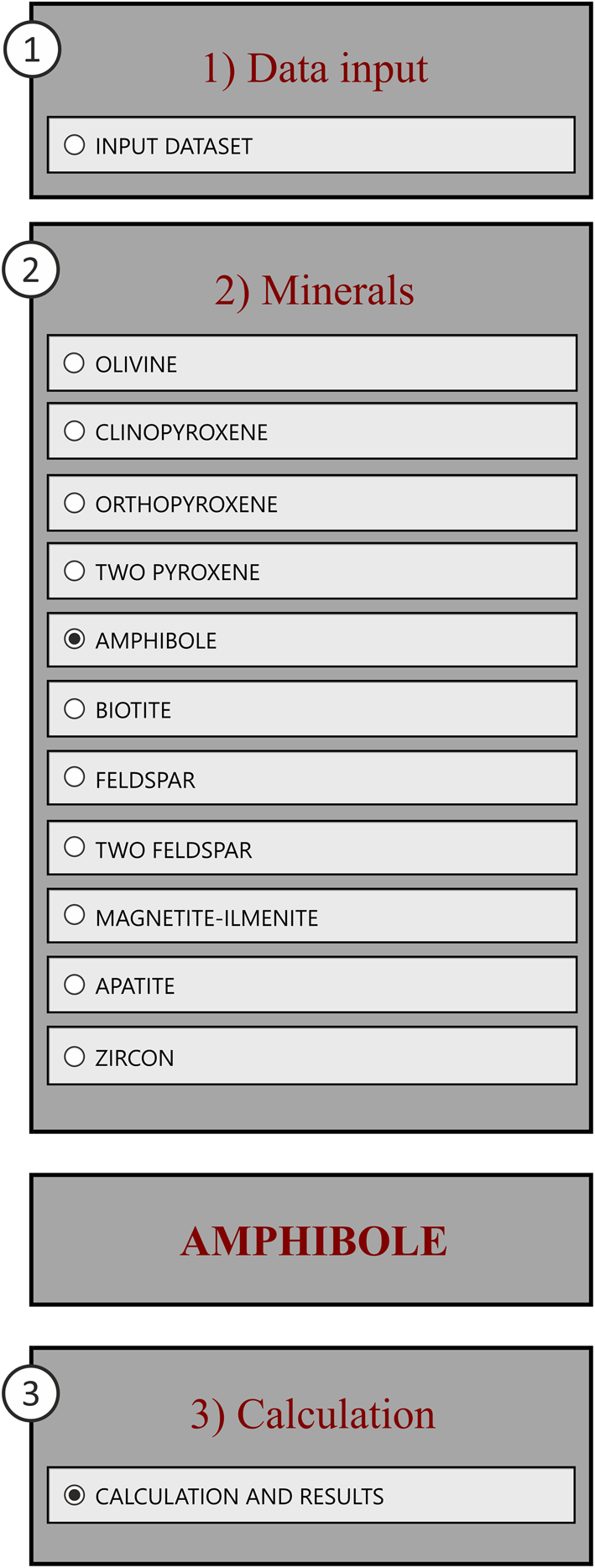
Fig. 2. The control panel for data entry which must be in the order of each mineral: 1) Data input, 2) Minerals, and 3) Calculation.
Olivine
Olivine is a ferromagnesian mineral represented by the two end-members of forsterite (Mg2SiO4) and fayalite (Fe2SiO4). Olivine compositions are recalculated on the basis of four oxygens and typically shown as molar percentages of forsterite (Fo) and fayalite (Fa) in the literature and also in MagMin_PT.
MagMin_PT calculates T (°C) from EPMA data using liquid thermometers (Helz and Thornber, Reference Helz and Thornber1987; Beattie, Reference Beattie1993; Sisson and Grove, Reference Sisson and Grove1993; Putirka et al., Reference Putirka, Perfit, Ryerson and Jacksond2007; Putirka, Reference Putirka, Putirka and Tepley2008). For the olivine–liquid thermometer, the composition of ‘whole rock’ or ‘glass’ needs to be entered in the ‘Data Input’ sheet. Then, the program calculates the Fe–Mg exchange coefficient or KD(Fe–Mg)ol–liq using equations 1 and 2 to test for equilibrium between olivine and liquid. If the entered liquid is under equilibrium with the olivine composition, this value is expected to be in the range of KD = 0.30 ± 0.03 (Roeder and Emslie, Reference Roeder and Emslie1970; Toplis, Reference Toplis2005), which means that the thermometer can be applicable to the volcanic system. The results are presented in the ‘Olivine’ sheet.
Pyroxene
This sheet designed for pyroxenes whose general chemical formula is M2M1T2O6. They are classified according to the occupancy of the M2 site, though Morimoto et al. (Reference Morimoto, Fabries, Ferguson, Ginzburg, Ross, Seifert, Zussman, Aoki and Gottardi1988) assumed the M1 and M2 sites were a single M site, because T, M1 and M2 sites are a function of temperature in pyroxenes (Yavuz, Reference Yavuz2013). In MagMin_PT, a pyroxene formula is recalculated on the basis of six oxygens according to the scheme of allocation of cations by Morimoto et al. (Reference Morimoto, Fabries, Ferguson, Ginzburg, Ross, Seifert, Zussman, Aoki and Gottardi1988) and the estimation of Fe3+ is made using the following equation given by Droop (Reference Droop1987):

where T is the ideal number of cations per formula unit, and S is the observed cation total per X oxygens calculated assuming all iron to be Fe2+.
In the ‘Data Input’ sheet in MagMin_PT, three different options exist for pyroxene data entry. One option is ‘Two pyroxene’ data under the heading ‘Minerals’, with results appearing in the ‘Pyroxene’ sheet. In this sheet, many classification diagrams (Morimoto and Kitamura, Reference Morimoto and Kitamura1983; Morimoto et al., Reference Morimoto, Fabries, Ferguson, Ginzburg, Ross, Seifert, Zussman, Aoki and Gottardi1988) and several two pyroxene geothermobarometers (Wood and Banno, Reference Wood and Banno1973; Wells, Reference Wells1977; Lindsley and Andersen, Reference Lindsley and Andersen1983; Brey and Köhler, Reference Brey and Köhler1990; Putirka, Reference Putirka, Putirka and Tepley2008) are produced (Fig. 3). Another option for data input is to enter ortho- and clinopyroxene data independently. This is especially useful for mineral–liquid geothermobarometry that requires calculations of the Fe–Mg exchange coefficient for orthopyroxene (KD(Fe–Mg)opx–liq) and clinopyroxene (KD(Fe–Mg)cpx–liq) to test for equilibrium between mineral–liquid pairs according to equation 2. KD values are expected to be in the range of 0.29 ± 0.06 for opx and 0.27 ± 0.03 for cpx to meet equilibrium conditions. The equilibrium tests are also graphically portrayed in a ‘Rhodes Diagram’ (Rhodes et al., Reference Rhodes, Dungan, Blanchard and Long1979) in the ‘Pyroxene’ sheet, resulting in a binary plot of 100×Mg# Liquid vs. 100×Mg# orthopyroxene or clinopyroxene. On such a plot, the equilibrated mineral–liquid pairs lie between two dashed lines marking error bounds.

Fig. 3. Plot of ortho- and clinopyroxene compositions (Deer et al., Reference Deer, Howie and Zussman1992) on the pyroxene isotherm curves (Lindsley and Andersen, Reference Lindsley and Andersen1983).
MagMin_PT also includes an equilibrium test for clinopyroxene in the ‘Pyroxene’ sheet, which is a comparison between predicted and observed values for the clinopyroxene components on a binary plot. Under equilibrium conditions, the predicted and observed values plot on, or close to, the one-to-one regression line.
Amphibole
Amphiboles are one of the most complex rock-forming double-chain inosilicates with a wide range of compositions, and are represented by a general formula of AB2C5T8O22W2. Amphibole classification has not been satisfactory since Leake (Reference Leake1968) presented the first classification for calcic amphiboles. New discoveries of amphibole compositions has led to many classification attempts in parallel with ongoing development in analytical techniques in the intervening years (e.g. IMA reports of Leake, Reference Leake1978; Leake et al., Reference Leake, Woolley, Arps, Birch, Gilbert, Grice, Hawthorne, Kato, Kisch, Krivovichev, Linthout, Laird, Mandarino, Maresch, Nickel, Rock, Schumacher, Smith, Stephenson, Ungaretti, Whittaker and Guo1997; Leake et al., Reference Leake, Woolley, Birch, Burke, Ferraris, Grice, Hawthorne, Kisch, Krivovichev, Schumacher, Stephenson and Whittaker2003; and Hawthorne et al., Reference Hawthorne, Oberti, Harlow, Maresch, Martin, Schumacher and Welch2012). These attempts have also been accompanied by the addition of new computer programs and spreadsheets to overcome classification problems resulting from the compositional complexity of amphiboles (e.g. Currie, Reference Currie1997; Yavuz, Reference Yavuz1999; Mogessie et al., Reference Mogessie, Ettinger, Leake and Tessadri2001; Esawi, Reference Esawi2004; Yavuz, Reference Yavuz2007; Locock, Reference Locock2014).
MagMin_PT converts the entered amphibole microprobe analysis in ‘Data Input’ to formula proportions in atoms per formula unit (apfu) in the ‘Amphibole’ sheet according to the IMA 2012 recommendations (Hawthorne et al., Reference Hawthorne, Oberti, Harlow, Maresch, Martin, Schumacher and Welch2012), which results in eight different binary classification diagrams (Fig. 4). MagMin_PT includes an alternative formula calculation scheme based on the machine learning method for Li-free and Li-bearing amphiboles by Li et al. (Reference Li, Zhang, Behrens and Holtz2020a). The users can compare their formula calculations between this new approach and IMA 2012. The Fe3+/Fe2+ ratio cannot be determined routinely by electron microprobe techniques therefore in MagMin_PT Fe3+ it is estimated empirically on the basis of the electroneutrality and stoichiometry rule. Further details on the Fe3+ calculations for IMA 2012 classification are given in Appendix III of Hawthorne et al. (Reference Hawthorne, Oberti, Harlow, Maresch, Martin, Schumacher and Welch2012).

Fig. 4. Classification diagram of calcic-amphibole according to IMA 2012 (Hawthorne et al., Reference Hawthorne, Oberti, Harlow, Maresch, Martin, Schumacher and Welch2012). Data set from Deer et al. (Reference Deer, Howie and Zussman1992).
MagMin_PT includes mineral–mineral (e.g. amphibole–plagioclase), mineral–liquid (e.g. amphibole–liquid) and single-phase amphibole (e.g. Al-in-hornblende) geothermobarometers proposed by different authors in the ‘Amphibole’ sheet. Al-in-hornblende calibrations are the most commonly used barometers based on EPMA-derived data. Several Al-in-hornblende barometers (Hammerstrom and Zen, Reference Hammerstrom and Zen1986; Hollister et al., Reference Hollister, Grissom, Peters, Stowell and Sisson1987; Johnson and Rutherford, Reference Johnson and Rutherford1989; Blundy and Holland, Reference Blundy and Holland1990; Schmidt, Reference Schmidt1992; Anderson and Smith, Reference Anderson and Smith1995) are included in the program. However, these barometers should be used with caution because they are valid only under restricted conditions, and so not generally applicable to igneous systems (Erdmann et al., Reference Erdmann, Martel, Pichavant and Kushnir2014; Putirka, Reference Putirka2016). Amphibole–plagioclase (Blundy and Holland, Reference Blundy and Holland1990; Holland and Blundy, Reference Holland and Blundy1994; Molina et al., Reference Molina, Moreno, Castro, Rodríguez and Fershtater2015; Molina et al., Reference Molina, Cambeses, Moreno, Morales, Montero and Bea2021) and amphibole–liquid (Molina et al., Reference Molina, Moreno, Castro, Rodríguez and Fershtater2015; Putirka, Reference Putirka2016) geothermobarometers require plagioclase and glass or whole-rock compositions to be entered into the program (lower right panel on Data Input sheet). The Fe–Mg exchange coefficient (KD(Fe–Mg)amp–liq) is expected to be in the range of 0.28 ± 0.11 for the amphibole–liquid thermobarometer.
The program also presents oxygen buffers constraining oxygen fugacity ($f_{\rm{O_2}}$ ) as a function of temperature (Fegley, Reference Fegley2012), and water content (%) of melt (Ridolfi et al., Reference Ridolfi, Renzulli and Puerini2010; Ridolfi, Reference Ridolfi2021) calculated from amphibole compositions.
Biotite
Biotites are trioctahedral micas characterised by end-members of KFe3AlSi3O10(OH)2 (annite), KMg3AlSi3O10(OH)2 (phlogopite), KFe2AlAl2Si2O10(OH)2 (siderophyllite) and KMg2AlAl2Si2O10(OH)2 (eastonite) (Rieder et al., Reference Rieder, Cavazzini, D'yakonov, Frank-Kamenetskii, Gottardi, Guggenheim, Koval’, Müller, Neiva, Radoslovich, Robert, Sassi, Takeda, Weiss and Wones1999). In MagMin_PT, the biotite formula is calculated on the basis of 11, 22 or 24 oxygens depending on user data (e.g. available of H2O analysis) and oxidation state of biotite, etc. Therefore, this can be done traditionally using Rieder et al. (Reference Rieder, Cavazzini, D'yakonov, Frank-Kamenetskii, Gottardi, Guggenheim, Koval’, Müller, Neiva, Radoslovich, Robert, Sassi, Takeda, Weiss and Wones1999), and Fe3+ can be calculated on the basis of the equations given by Dymek (Reference Dymek1983), though this may result in large errors in the estimations of Fe3+/ΣFe. The concentration of Li2O in biotites, if essential but not known, can be estimated using the empirical equations in the program (Tindle and Webb, Reference Tindle and Webb1990; Tischendorf et al., Reference Tischendorf, Gottesmann, Förster and Trumbull1997; Tischendorf et al., Reference Tischendorf, Förster and Gottesmann1999). Alternatively, MagMin_PT includes a new scheme for the biotite formula calculation and Fe3+ estimation based on a machine learning method by Li et al. (Reference Li, Zhang, Behrens and Holtz2020b). The program includes basic classification diagrams for biotites, and for micas to some extent. MagMin_PT also has options for P–T (Luhr et al., Reference Luhr, Carmichael and Varekamp1984; Uchida et al., Reference Uchida, Endo and Makino2007) calculations and oxygen buffers (Wones and Eugster, Reference Wones and Eugster1965; Wones, Reference Wones1989). Pressure–temperature calculations for biotites do not require whole-rock or glass analysis data because these are not liquid-based thermobarometers.
Feldspars
Feldspars are classified according to the end-members of the NaAlSi3O8 (albite, Ab) – CaAl2Si2O8 (anorthite, An) – KAlSi3O8 (orthoclase, Or) solid solution (after Deer et al., Reference Deer, Howie and Zussman1992). Compositions between Ab and An are referred to as plagioclases and those between Ab and Or as alkali feldspars (Fig. 5).
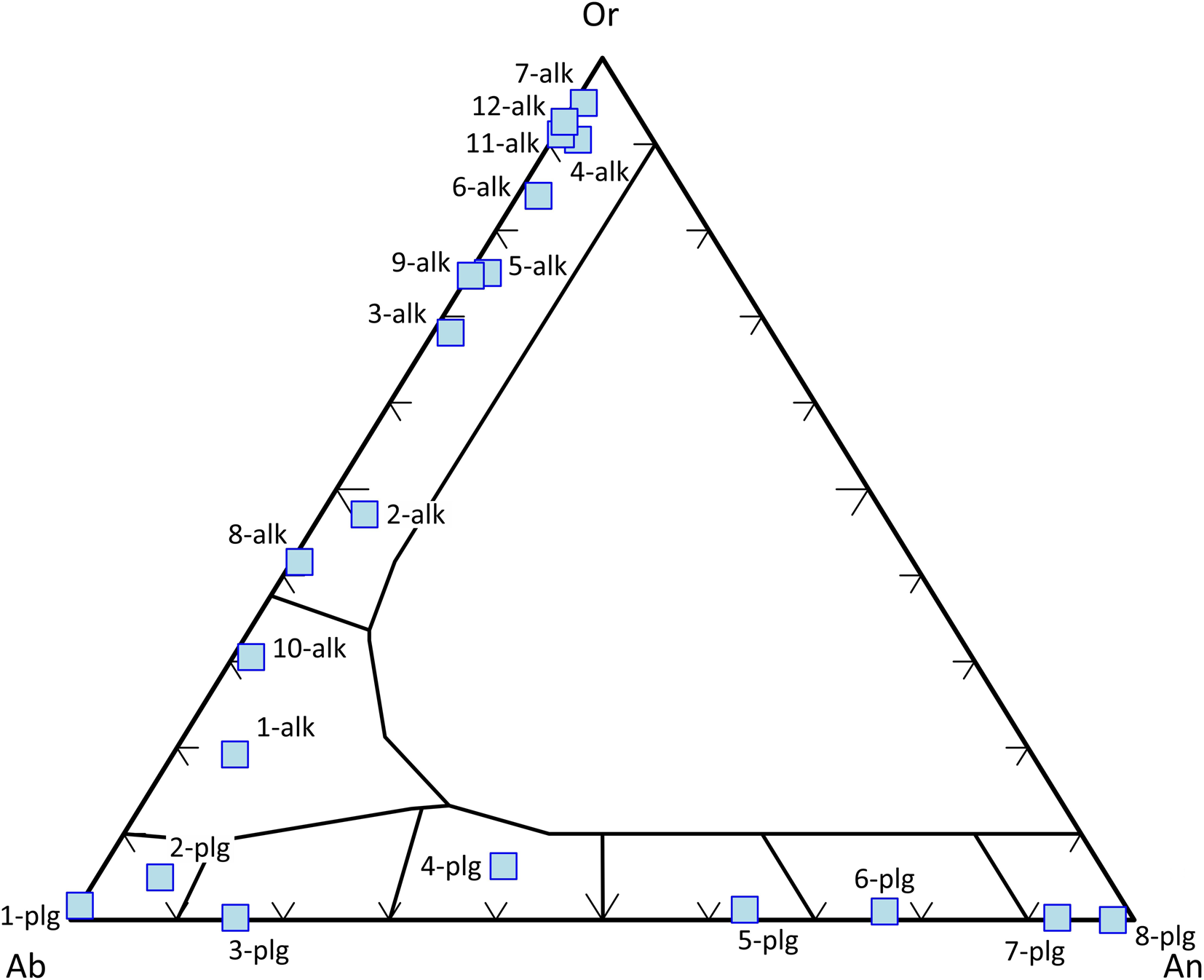
Fig. 5. Classification of feldspars according to the end-members of the Ab–An–Or ternary diagram. Data set from Deer et al. (Reference Deer, Howie and Zussman1992).
In MagMin_PT, the feldspar formula is recalculated on the basis of 8, 16 or 32 oxygens depending on user choice, allowing Ab–An–Or components to be calculated and plotted in the feldspar ternary diagram. The program includes several thermobarometers (e.g. plagioclase–liquid, alkali feldspar–liquid, two feldspar etc). For mineral–liquid thermobarometers, users should enter their whole-rock or glass composition into the ‘Data Input’ sheet, and then test for equilibrium between pairs on the basis of the Ab–An exchange coefficient (KD) using equation 4. The plagioclase–liquid equilibrium can also be used for a hygrometer, if the temperature is well-defined (Putirka, Reference Putirka2005, Reference Putirka, Putirka and Tepley2008). Thus, the program calculates H2O (wt.%) content of the liquid using results from the aforementioned hygrometer. MagMin_PT includes another water content (H2O wt.%) calculation procedure using the Al2O3 content of the melt as a hygrometer (P < 4 kbar) (Pichavant and Macdonald, Reference Pichavant and Macdonald2007), so that users can compare H2O results from two different calculations.

Magnetite–Ilmenite
Ilmenite and magnetite are generally termed as Fe–Ti oxides with the idealised formula of FeTiO3 and Fe3O4, respectively. Two major solid-solution series occur as ‘ulvöspinel–magnetite’ and ‘ilmenite–hematite’ in the FeO–Fe2O3–TiO2 system. The compositions of coexisting ilmenite and magnetite have been used extensively as a thermobarometer because their compositions are strongly dependent on ${f_{\rm{O_2}}}$ (oxygen fugacity) and the T at which they equilibrated.
In natural magmatic systems, there are several buffer reactions that magnetite is involved in that can be used to characterise the oxidation state of magmas, such as the hematite–magnetite (HM), the quartz–fayalite–magnetite (QFM), and the magnetite–wüstite (MW) reactions. The Nickel-Nickel Oxide (NNO) buffer reaction does not occur in natural magmas though is commonly used for reference. Log oxygen fugacity, an index of the redox state in a magma for each buffer assemblage was compiled by Frost (Reference Frost and Lindsley1991) and calculated from:

where T is temperature in Kelvin (K), P is pressure (bar), and A, B and C are buffers from equilibrium expressions according to Frost (Reference Frost and Lindsley1991).
Magnetite and ilmenite formulae are calculated on the basis of 4 and 3 oxygens, respectively in MagMin_PT. The calculation results are shown on ternary diagrams (e.g. FeO–Fe2O3–TiO2 or R2+–R3+–Ti4+). Fe3+ separation is according to the equation of Droop (Reference Droop1987). MagMin_PT calculates T (°C) and $f_{\rm{O_2}}$ values, calibrated by different researchers (Powell and Powell, Reference Powell and Powell1977; Spencer and Lindsley, Reference Spencer and Lindsley1981; Andersen and Lindsley, Reference Andersen and Lindsley1985; Sauerzapf et al., Reference Sauerzapf, Lattard, Burchard and Engelmann2008), and their results are plotted on a binary diagram with several buffer curves (e.g. MW, QFM, NNO and HM). Users can adjust the buffer curves of the HM and QFM as ‘low T’, ‘medium T’ or ‘high T’ according to their systems. The program presents another binary diagram of T (°C) vs. ΔNNO, which is the relative oxygen fugacity at given T for NNO.
A revised Fe–Ti oxide geothermometer and oxygen-barometer has been published by Ghiorso and Evans (Reference Ghiorso and Evans2008). This is based on a thermodynamic model that produces different results than older calibrations, most notably in the estimation of oxidation state under relatively oxidised conditions (>NNO + 1). This thermobarometry is not included in MagMin_PT, however users can find an icon in the ‘Magnetite-Ilmenite’ sheet redirecting them to a web-based application designed by these authors for the T (°C) and NNO calculations.
Apatite
Apatite, Ca5(PO4)3(F,Cl,OH), is a member of the group of phosphate minerals, and it is very common as an accessory phase in igneous rocks. MagMin_PT includes apatite formula (e.g. 25 or 26 oxygens) and saturation temperature calculations. Apatite saturation temperature (Piccoli et al., Reference Piccoli, Candela and Williams1999; Piccoli and Candela, Reference Piccoli, Candela, Kohn, Rakovan and Hughes2002) is calculated from whole-rock geochemical data that must be entered into the ‘Data Input’ sheet in the program.
Zircon
Zircon is an accessory orthosilicate with the formula of ZrSiO4. It is commonly found as early-formed small crystals enclosed in later minerals in magmatic rocks. When enclosed, especially in biotite or amphibole, pleochroic haloes resulting from radioactive element content (Th,U) can be observed optically around zircon (Deer et al., Reference Deer, Howie and Zussman1992).
MagMin_PT calculates zircon formulae on the basis of 4 oxygens. The program includes options for ‘zircon saturation temperature’ and ‘Ti-in-zircon thermometry’. Therefore, the saturation temperature of zircon (Hanchar and Watson, Reference Hanchar, Watson, Hanchar and Hoskin2003; Boehnke et al., Reference Boehnke, Watson, Trail, Harrison and Schmitt2013) can be calculated from the whole-rock chemistry with the parameters M [(Na + K + 2Ca)/(Al × Si)] of Watson and Harrison (Reference Watson and Harrison1983) and FM [(Na + K + (2Ca + Fe + Mg))/(Al × Si)] of Ryerson and Watson (Reference Ryerson and Watson1987). Additionally, Ti-in-zircon thermometry T (°C) of Watson et al. (Reference Watson, Wark and Thomas2006) can be calculated by the program and is included in the ‘Zircon’ spreadsheet.
Conclusions
MagMin_PT is an Excel© based, open, and free mineral classification and geothermobarometry program available in the Supplementary materials. The program processes EPMA data using new and conventional cation recalculation methods, which produces mineral classification diagrams and P–T data. The objective of this work is to provide a user friend Excel-based program using the latest developments for those investigating the mineral compositions and petrology of magmatic rocks. Finally, mineral classification diagrams, formulae proportions and geothermobarometry data can easily be exported as ‘gif/jpeg/tiff’ files and tables.
Acknowledgements
The authors thank the Principal Editor Roger Mitchell, Associate Editor Katharina Pfaff and two anonymous reviewers for their critical and constructive comments that improved the quality of this paper and MagMin_PT.
Competing interests
The authors declare none.
Supplementary material
To view supplementary material for this article, please visit https://doi.org/10.1180/mgm.2022.113


