


Introduction
The Ordovician and Silurian were intervals of tremendous evolutionary and environmental upheaval, encompassing both the great Ordovician biodiversification event (GOBE), and the onset and aftermath of the Late Ordovician mass extinction (LOME) (Webby et al. Reference Webby, Paris, Droser and Percival2004; Servais and Harper Reference Servais and Harper2018; Rasmussen et al. Reference Rasmussen, Kröger, Nielsen and Colmenar2019; Stigall et al. Reference Stigall, Edwards, Freeman and Rasmussen2019). This has inspired intensive study of Ordovician–Silurian diversity patterns, because of their potential to reveal the mechanisms underlying extinction and diversification (e.g., Sepkoski Reference Sepkoski1988; Miller and Connolly Reference Miller and Connolly2001; Webby et al. Reference Webby, Paris, Droser and Percival2004; Servais et al. Reference Servais, Owen, Harper, Kröger and Munnecke2010; Hautmann Reference Hautmann2014; Penny and Kröger Reference Penny and Kröger2019).
The GOBE had multiple global environmental drivers that were mediated by regional-scale processes, including carbonate platform development, biotic invasions, and latitudinal shifts due to tectonic movements (e.g., Kiessling et al. Reference Kiessling, Flügel and Golonka2003; Servais and Harper Reference Servais and Harper2018; Stigall Reference Stigall2018). The impact of these regional processes on diversity is exemplified by the eastern Baltic paleobasin. Over the Ordovician, Baltica experienced regional warming as it drifted from temperate to equatorial latitudes, accompanied by the development of an extensive, reef-bearing carbonate shelf (Dronov and Rozhnov Reference Dronov and Rozhnov2007; Kröger et al. Reference Kröger, Hints and Lehnert2017b). Baltoscandia also has an abundant, well-preserved Ordovician–Silurian fossil record combined with a well-characterized stratigraphy (e.g., Paškevičius Reference Paškevičius1997; Raukas and Teedumäe Reference Raukas and Teedumäe1997; Ebbestad et al. Reference Ebbestad, Wickström and Högström2007; Calner et al. Reference Calner, Ahlberg, Lehnert and Erlström2013; Bauert et al. Reference Bauert, Hints, Meidla and Männik2014). This makes it an excellent focus for investigating how the environmental heterogeneity associated with carbonate shelf development influenced regional diversity patterns through the GOBE and LOME, as well as the impact of temporal turnover on these patterns.
Early Paleozoic Baltoscandian richness curves are available for several clades (e.g., Hammer Reference Hammer2003; Kaljo et al. Reference Kaljo, Hints, Hints, Männik, Martma and Nõlvak2011), but we follow other workers (e.g., Hints and Harper Reference Hints and Harper2003; Rasmussen et al. Reference Rasmussen, Hansen and Harper2007, Reference Rasmussen, Nielsen and Harper2009; Lam and Stigall Reference Lam and Stigall2015; Hints et al. Reference Hints, Harper and Paškevičius2018) in focusing on brachiopods. The taxonomy and biostratigraphy of Baltoscandian brachiopods have been studied by generations of specialists, such as Armin Öpik, Tatjana N. Alikhova, Arvo Rõõmusoks, Madis Rubel, Linda Hints, and Petras Musteikis (for recent reviews, see Harper et al. Reference Harper, Zhan and Jin2015; Harper and Hints Reference Harper and Hints2016). Because they are a major component of the early Paleozoic benthos, brachiopods are also a good model clade for investigating the impact of substrate changes on benthic diversity.
Here, we quantify how temporal turnover and environmental heterogeneity contributed to brachiopod diversification in the eastern part of the Baltic paleobasin during the GOBE and also to the recovery after the LOME.
Geologic and Depositional Setting
During the early Paleozoic, the Baltic paleobasin was an extensive epicontinental sea of the Baltica paleocontinent. The extent and development of the Baltic paleobasin was closely related to the Baltic Syneclise, a tectonic structure with a roughly 700-km-long southwest–northeast oriented long axis (Tuuling Reference Tuuling2019) (Fig. 1). During the Cambrian–Silurian, Baltica underwent a plate-tectonic shift from temperate to equatorial latitudes (Torsvik and Cocks Reference Torsvik and Cocks2016), with a corresponding shift in regional sediment deposition from cool-water glauconitic carbonates and siliciclastics to reduced siliciclastic input and tropical carbonates (Torsvik et al. Reference Torsvik, Smethurst, Meert, Van der Voo, McKerrow, Brasier, Sturt and Walderhaug1996; Cocks and Torsvik Reference Cocks and Torsvik2005; Dronov and Rozhnov Reference Dronov and Rozhnov2007) (Fig. 2).
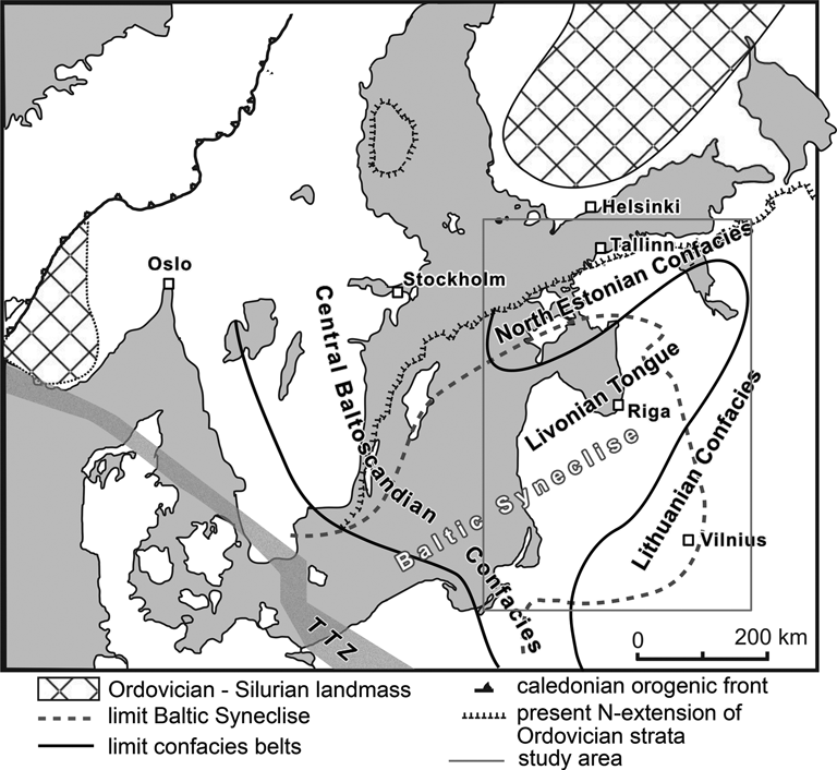
Figure 1. Regional facies map, showing confacies belts of the Baltic paleobasin and the extent of the Baltic Syneclise. TTZ, Teisseyre-Tornquist Zone. Compiled from Jaanusson (Reference Jaanusson1976), Lazauskiene et al. (Reference Lazauskiene, Sliaupa, Brazauskas and Musteikis2003), and Tuuling (Reference Tuuling2019). The study region is outlined with a gray square.

Figure 2. Overview of brachiopod localities with lithologic information used in this study. Maps show extent of outcrop and subcrop of strata of the respective time bins. Hatched lines show facies boundaries. Maps are adopted from Paškevičius (Reference Paškevičius1997: O1, Tremadoc, fig. 41; O2, Latorp, fig. 42; O4, Kunda, fig. 43; O5, Kukruse, fig. 44; O6, Oandu, fig. 45; O7, Ashgill, fig. 47; S1, Raikküla, fig. 59; S2, Adavere, fig. 60; S4, Ludlow, fig. 62; S5, Pridoli, fig. 63) and Raukas and Teedumäe (Reference Raukas and Teedumäe1997: O3, Volkhov, fig. 142). 1, brachiopod locality with lithologic information; 2, reef occurrence; 3, boundary between our “basinal,” “platform” areas; 4, facies boundary; 5, no time-bin sediments preserved; 6, extent of time-bin sediments.
During the Middle and Late Ordovician, the Baltic paleobasin differentiated into shelf and basin facies zones (Fig. 3). Jaanusson (Reference Jaanusson1976) distinguished a series of depositional zones, among others the Livonian Basin in the easternmost center of the basin and the North Estonian and Lithuanian Confacies belts as horseshoe-like marginal zones (Fig. 1). The most distal of these is the Scanian Confacies belt in the extreme southwest of the basin comprising parts of modern Denmark and Poland, which is dominated by graptolitic shales.

Figure 3. North–south cross sections showing facies distribution through the northern flank of the Baltic Basin from western Estonia in the north to western Lithuania in the south. Vertical lines mark locations of drill-core sections and the distributions of different lithologies. A, Silurian strata; based on Nestor and Einasto (Reference Nestor, Einasto, Kaljo and Klaamann1982). B, Ordovician strata; based on Dronov et al. (Reference Dronov, Ainsaar, Kaljo, Meidla, Saadre, Einasto, Gutiérrez-Marco, Rábano and García-Bellido2011). Roman numerals identify depositional intervals sensu Nestor and Einasto (Reference Nestor, Einasto, Raukas and Teedumäe1997).
The spatiotemporal development of the Baltic paleobasin is divided into five stages that are distinct with respect to tectonic subsidence rate, climate, large-scale eustatic sea-level trend, and differences in relative influx and production of siliciclastics and carbonates (Einasto and Nestor Reference Einasto and Nestor1973; Nestor and Einasto Reference Nestor, Einasto and Kaljo1977, Reference Nestor, Einasto, Raukas and Teedumäe1997; Einasto Reference Einasto, Radionova, Einasto, Kaljo and Klaaman1986). The first two stages, the (1) transgression and (2) unification stages, are equivalent to a ramp situation, with a gently dipping seafloor slope, relatively low spatial facies differentiation, and very slow depositional rates. The last three stages, the (3) differentiation, (4) stabilization, and (5) infilling stages, correspond to a carbonate platform situation with high carbonate depositional rates, high spatial bathymetric differentiation, phases of aggregation and progradation, and eventual termination. The change between the ramp and the platform situation was relatively abrupt and occurred at around the Sandbian/Katian stage boundary during the regional Keila–Oandu stages (see also Hints et al. Reference Hints, Meidla, Nõlvak and Sarv1989; Nestor and Einasto Reference Nestor, Einasto, Raukas and Teedumäe1997).
The late Sandbian–early Katian change from ramp to platform depositional settings coincided with a drastic inversion in wind and water currents (Kiipli et al. Reference Kiipli, Kiipli, Kallaste, Hints, Somelar and Kirsimäe2007) and a turnover in the biota (Ainsaar et al. Reference Ainsaar, Meidla and Martma2004). This occurred alongside the first widespread development of reefs (Kröger et al. Reference Kröger, Ebbestad and Lehnert2016) and the development of an algal-rich micritic limestone facies (Kröger et al. Reference Kröger, Penny, Shen and Munnecke2020). The massive increase in carbonate production was probably the main cause for the establishment of a stable, widespread, flat-topped carbonate platform and the consequent development of an extensive Ordovician–Silurian facies mosaic (in the sense of Wright and Burgess Reference Wright and Burgess2005). The different carbonate platform substrates include: extensive hardground development (Orviku Reference Orviku1940; Saadre Reference Saadre1993; Dronov et al. Reference Dronov, Meidla, Ainsaar and Tinn2000; Vinn and Wilson Reference Vinn and Wilson2010), shallow and lagoonal soft sediments (e.g., Einasto Reference Einasto, Radionova, Einasto, Kaljo and Klaaman1986; Teller Reference Teller1997), a micritic limestone with abundant calcareous algae (Spjeldnæs and Nitecki Reference Spjeldnæs and Nitecki1994; Kröger et al. Reference Kröger, Penny, Shen and Munnecke2020), kilometer-wide shoal deposits of echinoderm grainstone, and reefs and mud-mounds (e.g., Aaloe and Nestor Reference Aaloe, Nestor and Kaljo1977; Tuuling and Flodén Reference Tuuling and Flodén2013; Kröger et al. Reference Kröger, Hints, Lehnert, Männik and Joachimski2014, Reference Kröger, Ebbestad and Lehnert2016; Kaminskas et al. Reference Kaminskas, Michelevičius and Blažauskas2015).
Hirnantian diamictites exposed in Poland demonstrate that icebergs reached the western margin of Baltica, despite its position at subtropical latitudes (Porębski et al. Reference Porębski, Anczkiewicz, Paszkowski, Skompski, Kędzior, Mazur, Szczepański, Buniak and Mikołajewski2019). Carbonate deposition continued through the Hirnantian and into the Silurian, with ongoing high levels of facies differentiation between shallow-marine carbonate-rich and distal siliciclastic settings (Kiipli et al. Reference Kiipli, Kiipli and Kallaste2004).
Methods
Data, Downloads, and Data Cleaning
We used combined brachiopod fossil occurrence data from the literature-based Paleobiology Database (PBDB, https://paleobiodb.org) and from the specimen-level database of the Geoscience Collections of Estonia (SARV, https://geocollections.info; Hints et al. Reference Hints, Isakar and Toom2019), comprising a dataset of more than 13,000 occurrences from more than 800 localities in the eastern Baltic paleobasin (Estonia, Latvia, and Lithuania) (downloaded 13 January 2020). Brachiopod occurrences from the combined databases are mapped in Figure 2. Because the PBDB and SARV databases use different “collection” concepts, we assigned all occurrences to artificial collections, wherein a “collection” comprises all brachiopod occurrences within a lithostratigraphic unit at a single location, with location coordinates matched at a precision of three decimal places.
Lithologic and stratigraphic data were obtained from data associated with the PBDB and SARV occurrences, from a separate download of drill-core data compiled within the SARV, and from our own compilation from the literature. Only brachiopod occurrences identified to genus or species level were used for the analysis. Lithostratigraphic units of formation, member, and bed level were used. The hierarchy of the lithostratigraphic units, and in some cases their names, changed over the historical course of stratigraphic research. We corrected manually for historical name changes. Because we aimed to get a proxy for spatial and temporal lithologic heterogeneity, we flattened the hierarchy of lithologic names and considered each name as reflecting a distinct lithostratigraphic unit with equal value. Sequence boundaries were taken from Nielsen (Reference Nielsen, Webby, Paris, Droser and Percival2004), Johnson (Reference Johnson2006), and Dronov et al. (Reference Dronov, Ainsaar, Kaljo, Meidla, Saadre, Einasto, Gutiérrez-Marco, Rábano and García-Bellido2011).
Time Bins
The Ordovician and Silurian strata of the eastern Baltic paleobasin were divided into 12 time bins with an average duration of 5.6 Myr (Fig. 4). The shortest time bin is S5 (3.8 Myr) and the longest is O4 (8.3 Myr). Time binning was based on well-resolved stratigraphic horizons and reflects a compromise between time resolution and available data. Absolute ages of time-bin boundaries were taken from Gradstein et al. (Reference Gradstein, Ogg, Schmitz and Ogg2012) and Lindskog et al. (Reference Lindskog, Costa, Rasmussen, Connelly and Eriksson2017).

Figure 4. Stratigraphic scheme showing time binning, depositional cycles, and stages of the depositional model for the Baltic paleobasin. Compiled from Gradstein et al. (Reference Gradstein, Ogg, Schmitz and Ogg2012), Männik (Reference Männik2014), and Lindskog et al. (Reference Lindskog, Costa, Rasmussen, Connelly and Eriksson2017) for absolute time; Kiipli et al. (Reference Kiipli, Kiipli, Kallaste and Märss2016, Reference Kiipli, Kiipli, Kallaste and Pajusaar2017) for climate; Calner (Reference Calner and Elewa2008) and Rasmussen et al. (Reference Rasmussen, Kröger, Nielsen and Colmenar2019) for bio-events; Nielsen (Reference Nielsen, Webby, Paris, Droser and Percival2004), Johnson (Reference Johnson2006), and Dronov et al. (Reference Dronov, Ainsaar, Kaljo, Meidla, Saadre, Einasto, Gutiérrez-Marco, Rábano and García-Bellido2011) for depositional cycles; Nestor and Einasto (Reference Nestor, Einasto, Raukas and Teedumäe1997) for depositional intervals. H, humid interval. Stage abbreviations: Daping., Dapingian; Hirn., Hirnantian; Rhudd., Rhuddaninan; Aer., Aeronian; Shein., Sheinwoodian; Hom., Homerian; Gor., Gorstian; Ludf., Ludfordian.
The Silurian record of the eastern Baltic paleobasin is included for several reasons. By including more time bins, we could track the relationships between regional diversity and substrate change from the initiation of the carbonate shelf in the Baltic paleobasin to the eventual infilling of the paleobasin in the late Silurian–Early Devonian. This encompasses more change in substrates and biodiversity and also provides points of comparison for the Ordovician data, allowing evaluation of the influence of time-specific biodiversity change and regional spatial and facies effects.
Identifying Biogenic Lithologies
We classified lithostratigraphic units into either (1) bio-dominated lithologies comprising carbonates of primarily organismic origin; and (2) non–bio-dominated lithologies comprising predominantly siliciclastic sediments and chemical sedimentary rocks. In the first category are all limestone lithologies, including marly, argillaceous, silty, dolomitic, and glauconitic limestone. In the second category are shale, marl, siltstone, sandstone, glauconite, dolomite, and gypsum lithologies. For simplicity, we call the bio-dominated category “carbonate-dominated” and the non–bio-dominated category “siliciclastic-dominated,” although dolomites are also carbonates, and gypsum is not siliciclastic. We include a list of lithostratigraphic units and their designations as carbonate and siliciclastic dominated in Supplementary Material 1. Time bin S2 was excluded from some analyses, because the only carbonate-dominated lithostratigraphic unit it contains is the Rumba Formation, which contains a very low diversity assemblage dominated by a single genus, which sometimes causes the mean diversity to decline at higher hierarchical levels (see “Diversity Partitioning” section for details of the hierarchical partitions).
Diversity Partitioning
We use the term “richness” to refer to the number of genera (which may be a raw count or an estimate based on some form of standardization) and “diversity” as an umbrella term when referring to diversity measures in the Hill number family. These include richness, but also the Shannon and Simpson diversities, which are the Shannon and Simpson indices converted to their corresponding Hill numbers (terminology after Hsieh et al. Reference Hsieh, Ma and Chao2016). “Alpha diversity” refers to diversity within hierarchically partitioned categories, “beta diversity” refers to diversity difference between categories, and “gamma diversity” refers to the regional diversity; each may be measured with any of the three diversity measures used in this study. Where we refer to alpha, beta, or gamma diversity in only one of the diversity measures, we use the Greek letter with a subscript (e.g., γS is regional diversity, measured with richness; γshan and γsim would give the corresponding Shannon and Simpson diversities, respectively). All analyses were performed at the genus level.
Total (gamma) diversity can be partitioned into alpha and beta diversity using either additive or multiplicative approaches. While alpha and gamma diversity have the same meanings in both additive and multiplicative diversity partitioning, they differ in their concepts of beta diversity (which is also calculated using a range of other methods; reviewed in Koleff et al. Reference Koleff, Gaston and Lennon2003). In multiplicative diversity partitioning, beta diversity is the ratio of gamma diversity to alpha diversity (Koleff et al. Reference Koleff, Gaston and Lennon2003; Whittaker Reference Whittaker1972), while in additive diversity partitioning, beta diversity is gamma diversity minus alpha diversity (Lande Reference Lande1996).
Both diversity partitioning approaches can be used in hierarchical sampling schemes, which assign samples to progressively larger nested groups to assess how much diversity is contributed at each level. Hierarchical partitioning is readily applicable to fossil assemblages, because hierarchical sampling mirrors the hierarchical nature of lithostratigraphic and chronologic units (Patzkowsky and Holland Reference Patzkowsky and Holland2012). In hierarchical additive partitioning, beta diversity is the difference between the pooled diversity of a group of samples at a given hierarchical level and the mean alpha diversity of the samples that have been pooled (Lande Reference Lande1996). In hierarchical multiplicative diversity partitioning, beta diversity is the pooled diversity at a given hierarchical level divided by the mean diversity of its component samples (Jost et al. Reference Jost, DeVries, Walla, Greeney, Chao and Ricotta2010).
Additive diversity partitioning is sometimes preferred over multiplicative diversity partitioning, because it yields beta-diversity values in the same units as alpha and gamma diversity (e.g., Patzkowsky and Holland Reference Patzkowsky and Holland2007; Holland Reference Holland2010). Holland (Reference Holland2010) also advocated using three indices of diversity in parallel—richness, the Shannon index (also called the Shannon entropy), and the Simpson index (also called the Gini-Simpson index)—to evaluate diversity patterns in common and rare taxa and to control for the fact that richness is highly sensitive to sample size (Magurran Reference Magurran2004). Richness, being a simple count of the taxa in an assemblage, gives equal weight to all taxa, and consequently may be strongly influenced by the rarest taxa in an assemblage, as most of the species in a community tend to occur at low abundance (Whittaker Reference Whittaker1970; Reddin et al. Reference Reddin, Bothwell and Lennon2015). The Simpson index is most strongly influenced by the commonest taxa in an assemblage, which are arguably the most ecologically important (Gaston Reference Gaston2010), while the Shannon index has an intermediate sensitivity (for a full explanation, see Jost Reference Jost2007; Jost et al. Reference Jost, DeVries, Walla, Greeney, Chao and Ricotta2010).
However, the Shannon and Simpson indices do not behave additively and can give misleading results (Jost et al. Reference Jost, DeVries, Walla, Greeney, Chao and Ricotta2010). The solution, proposed by Jost et al. (Reference Jost, DeVries, Walla, Greeney, Chao and Ricotta2010), is to convert each index to its corresponding Hill number (Hill Reference Hill1973), also called its “effective number of species,” which is the number of species corresponding to the given diversity index when the species abundance distribution is perfectly even. These values can easily be compared with richness, because their units are the same.
After conversion to Hill numbers, the Shannon and Simpson indices yield the same within-group diversities whether partitioned multiplicatively or additively (Ricotta Reference Ricotta2005; Jost et al. Reference Jost, DeVries, Walla, Greeney, Chao and Ricotta2010). In this study, we used hierarchical multiplicative diversity partitioning with Hill numbers, because it yields the same within-category diversities as additive diversity partitioning and is easier to implement using the R package vegan (Oksanen et al. Reference Oksanen, Blanchet, Friendly, Kindt, Legendre, McGlinn, Minchin, O'Hara, Simpson, Solymos, Stevens, Szoecs and Wagner2018). However, in places we have expressed the differences in mean alpha diversity between hierarchical levels as a percentage of gamma diversity; this is not strictly equivalent to hierarchical additive diversity partitioning, but we use it as an additional, intuitive indicator of faunal difference between sampling units.
We used the function multipart, within the R package vegan (Oksanen et al. Reference Oksanen, Blanchet, Friendly, Kindt, Legendre, McGlinn, Minchin, O'Hara, Simpson, Solymos, Stevens, Szoecs and Wagner2018), to perform multiplicative diversity partitioning using the Tsallis entropy, with scale factors 0, 1, and 2 corresponding to taxonomic richness, Shannon index, and Simpson index. The resulting alpha and gamma diversities are given as their corresponding Hill numbers; we refer to these as the richness, Shannon diversity, and Simpson diversity, following Hsieh et al. (Reference Hsieh, Ma and Chao2016).
Data from 177 lithostratigraphic units were analyzed, of which 38 contain only a single collection. To avoid discarding these lithostratigraphic units, we present the raw data for all lithostratigraphic units containing five occurrences or more. We include coverage-standardized results, which show a substantially similar pattern, in Supplementary Material 2. Coverage was measured using Good's u (Good Reference Good1953), using a method from Alroy (Reference Alroy2014) as implemented by Brocklehurst et al. (Reference Brocklehurst, Day and Fröbisch2018). We coverage-standardized each lithostratigraphic unit to a Good's u of 0.5, a value chosen to maximize the number of time bins that would run. Lithostratigraphic units with lower coverage were discarded, and those whose coverage was higher were subsampled until the standardization coverage was reached. Subsampling was repeated 100 times for each time bin, and the mean diversities and associated p-values from null modeling recorded. Increasing the number of subsampling runs had a minimal effect on the results. We used the null modeling function in multipart to perform individual-based randomization, which randomly assigns occurrences to samples at the lowest level of the hierarchy and assesses whether the diversities in the sample are significantly different from those of the randomized data. Null models were run with 99 iterations for each subsampling run, and when reporting results, we focus our discussion on alpha and beta diversities with mean p-values < 0.1.
We used environmental partitioning to evaluate how faunal differences between lithologies contributed to regional diversity patterns, which relates to the influence of environmental preference and substrate heterogeneity on assemblage heterogeneity. The basic sample for alpha-diversity calculation was the lithostratigraphic unit, approximately equivalent to a formation. Formations have been taken to represent metacommunities, and hence may be ecologically meaningful units (Hofmann et al. Reference Hofmann, Tietje and Aberhan2019). We used a three-level hierarchy, with lithostratigraphic units nested within carbonate-dominated or siliciclastic-dominated lithologies, with the highest hierarchical level being the whole study region. We also evaluated beta diversity within siliciclastic- and carbonate-dominated lithologies by performing separate two-level partitions of siliciclastic- and carbonate-hosted diversity. Where we suspected that time binning might be affecting the diversity curves produced, we performed secondary analyses at stage-level temporal resolution.
For temporal diversity partitioning, we used a three-level hierarchy to evaluate how faunal turnover between stages contributed to the diversity curve. Again, we used lithostratigraphic units as the basic units for alpha-diversity calculation, followed by within-stage and within–time bin diversity. Brachiopod occurrences lacking stage level temporal resolution were excluded from this analysis.
We also performed diversity partitioning within shelf and basin facies. Brachiopod occurrences were assigned to shelf or basin facies based on their geographic locations; the R package icosa (Kocsis Reference Kocsis2017) was used to generate hexagonal equal-area grids of ~37 km per side, and occurrences were assigned to grids using the locate() function. The resulting grids were used as the sampling unit and were overlain on a facies map of the Baltic region to assign them to the shelf or basin facies for analysis. Comparison of shelf and basin diversity patterns covers the time interval from bin O6 onward, as this is when the platform differentiation phase began (Fig. 4).
The meanings of different diversities within the partitioning schemes are summarized in Table 1. Alpha, beta, and gamma diversity are referred to by their Greek characters, with subscripts denoting richness, Shannon diversity, or Simpson diversity.
Table 1. Meanings of different diversity terms used in the hierarchical partitions.

Independent Gamma-Diversity Estimates
In the hierarchical diversity partitioning analyses, coverage may vary between time bins. To estimate the richness trajectory through time, we used independently calculated richness curves produced using two methods. First, we used the estimateD function in the R package iNEXT (Hsieh et al. Reference Hsieh, Ma and Chao2016), standardizing to a coverage of 0.7, which is the maximum coverage at which time bins O3–S5 will run. Second, we used the capture–recapture (CR) modeling approach (Nichols and Pollock Reference Nichols and Pollock1983; Liow and Nichols Reference Liow and Nichols2010) by fitting the Jolly-Seber model following the POPAN formulation (Schwarz and Arnason Reference Schwarz and Arnason1996; see also Kröger et al. [Reference Kröger, Franeck and Rasmussen2019] for details of the method). We also produced coverage-standardized and CR modeling approach richness curves at stage-level temporal resolution to visualize how the time binning might influence richness trajectories, excluding stages without occurrences or where the estimateD function suggested large prediction bias. Because different methods can be expected to produce different richness estimates, we focus our discussion on trends in the data rather than absolute values. To determine whether carbonate-dominated and siliciclastic-dominated lithologies showed the same diversity patterns, we calculated independent coverage-standardized richness curves for each lithologic category.
Occupancy as an Abundance Proxy
In our study, direct brachiopod abundance data were not available. We therefore use the number of localities with occurrences as a rough proxy of abundance with the a priori assumptions that detection in the fossil record is, at least in part, dependent on abundance and that more-abundant species have higher occupancies (see e.g., Gaston et al. Reference Gaston, Blackburn, Greenwood, Gregory, Quinn and Lawton2000).
Results
Regional Richness (γS) over the Ordovician–Silurian
The GOBE and LOME are expressed in the regional richness patterns derived from CR (Fig. 5). With stage-level resolution, γS increases in two pulses, one in the Floian–early Dapingian (Billingen–Kunda regional stages), with a second, larger pulse in the Sandbian. The γS decline during time bin O7 is an effect of the time-binning strategy used, and with stage-level resolution, γS continues to increase up until the Porkuni (Fig. 5) and then abruptly declines into the Silurian, with only a limited recovery. The LOME is not preceded by a diversity loss and instead represents a relatively abrupt diversity decline between the Porkuni and Juuru regional stages.

Figure 5. Regional gamma-diversity curve based on CR modeling at time-bin and stage temporal resolution. Black ovals and solid line, gamma diversity at time-bin resolution; gray rectangles and dotted line, gamma diversity at stage resolution. Use of longer time bins masks the two pulses of regional diversification visible at the stage level and also shifts the apparent regional diversity peak to the Katian (O6 bin), whereas with stage-level temporal resolution, the peak is in the Porkuni stage (Hirnantian; O7 bin). Stage abbreviations are: Dp., Dapingian; Sand., Sandbian; Hi, Hirnantian; R., Rhuddanian; Ae., Aeronian; Tel., Telychian; Sh., Sheinwoodian; H., Homerian; G., Gorstian; L., Ludfordian; Pri., Pridoli.
Temporal Taxonomic Turnover
Taxonomic turnover between regional stages, β2 in our temporal partitioning scheme, is a major contributor to within-bin diversity, though its impact is highly dependent on the length of time bins and the diversity index used (Fig. 6). The Sandbian–Katian (time bin O6) is particularly strongly influenced by this effect (Fig. 6B,C), though it is reduced when using the Shannon and Simpson diversities (Table 2).

Figure 6. Temporal diversity partitioning, which emphasizes the contribution of temporal turnover to regional diversity. Curves are calculated using genus richness and Hill numbers corresponding to the Shannon and Simpson indices (Shannon and Simpson diversity). A three-level hierarchy is used, with mean diversity within lithostratigraphic units (alpha1, gray diamonds), mean diversity in regional stages within a time bin (alpha2, white diamonds), and regional diversity (gamma, black circles). The difference between alpha1 and alpha2 reflects the extent of faunal differences between lithostratigraphic units within regional stages, while the difference between alpha2 and gamma reflects faunal differentiation between regional stages. A, Raw genus richness curves. B, Shannon diversity curves. C, Simpson diversity curves. Stage abbreviations are: Dp., Dapingian; Sand., Sandbian; Hi, Hirnantian; R., Rhuddanian; Ae., Aeronian; Tel., Telychian; Sh., Sheinwoodian; H., Homerian; G., Gorstian; L., Ludfordian; Pri., Pridoli.
Table 2. Taxonomic turnover between stages (β2) measured as a percentage of γ diversity and the associated p-values. β2 was measured using richness, the Shannon diversity, and the Simpson diversity. The values used to produce this table are given in Supplementary Material 3A. Data where p-values were below 0.1 are highlighted in gray. NAs denote time bins with insufficient data for analysis, or where bins were not subdivided into multiple stages.

Environment-Specific Diversity Trajectories
As the Estonian and Lithuanian shelves developed, they created broadscale substrate heterogeneity in the eastern Baltic paleobasin, and differentiation between shallow-water and deep-marine facies. Shelfal localities typically have higher richness than basinal ones, and platform and basin facies also show distinct richness trends (Fig. 7).

Figure 7. Diversity partitioning in platform and basinal localities, defined based on the regional facies boundaries in Fig. 1. Diversity curves are only shown from O6 onward, as this marks the start of the platform differentiation depositional interval (Fig. 3). A two-level hierarchy is used, with genus richness within lithostratigraphic units (gray diamonds) and regional richness in the relevant setting (black circles). A large difference between the two diversity curves represents a larger contribution from beta diversity. Error bars represent 95% confidence intervals, though these are generally very small. A, Raw genus richness in platform environments. B, Raw genus richness in basinal environments. Stage abbreviations are: Hi, Hirnantian; R., Rhuddanian; Ae., Aeronian; Tel., Telychian; Sh., Sheinwoodian; H., Homerian; G., Gorstian; L., Ludfordian; Pri., Pridoli.
Differences in richness trajectories between shelf and basin are also reflected in differences in the diversity trajectories of carbonate- and siliciclastic-dominated lithologic categories, as carbonate-dominated lithologies predominantly occur on the shelf, at least after the Early Ordovician (Fig. 3). Independent richness curves for carbonate- and siliciclastic-dominated lithologies (Fig. 8) indicate that in the Ordovician, carbonate lithologies typically hosted higher richness than siliciclastic ones. However, parallel increases in carbonate- and siliciclastic-hosted richness over the Ordovician may suggest diversification drivers that operated across depositional environments. Siliciclastic-dominated lithostratigraphic units show a more rapid diversification than carbonate-dominated ones (Fig. 8) but are dominated by just a few brachiopod genera until O5 (Uhaku–Haljala stages, Darriwilian–Sandbian) (see Supplementary Material 3). The marked increase in siliciclastic-hosted richness in O6 reflects the regional faunal turnover event during this interval (Ainsaar et al. Reference Ainsaar, Meidla and Martma2004 and references therein).

Figure 8. Independent coverage-standardized genus richness curves for carbonate- and siliciclastic-dominated lithostratigraphic units, calculated using iNEXT, using both the regional stages (gray rectangles, dotted line) and coarser time-binning (black ovals, solid line) scheme. All curves are coverage-standardized to 0.7. A, Regional genus richness in carbonate-dominated lithologies. B, Regional genus richness in siliciclastic-dominated localities. Stage abbreviations are: Dp., Dapingian; Sand., Sandbian; Hi, Hirnantian; R., Rhuddanian; Ae., Aeronian; Tel., Telychian; Sh., Sheinwoodian; H., Homerian; G., Gorstian; L., Ludfordian; Pri., Pridoli.
With stage-level temporal resolution, carbonate- and siliciclastic-hosted richness curves are decoupled beginning during the Katian, during the Oandu Stage (in bin O6), and continuing into the Silurian (Fig. 8). In the Silurian, siliciclastic-hosted brachiopod richness begins to recover from the LOME earlier than carbonate-hosted richness, though both decline toward the end of the Silurian (Fig. 9). However, richness within carbonate-dominated lithologies closely reflects the regional richness pattern, suggesting that carbonate lithologies are dominating the regional richness trajectory, particularly in the Ordovician (compare Figs. 5 and 8A).

Figure 9. Lithologic diversity partitioning, which emphasizes how faunal differences between lithostratigraphic units contribute to regional diversity. Diversity curves were calculated using genus richness and Hill numbers corresponding to the Shannon and Simpson indices. A three-level hierarchy is used, with mean diversity within lithostratigraphic units (alpha1, gray diamonds), mean diversity within carbonate- and siliciclastic-dominated lithostratigraphic units (alpha2, white diamonds), and regional diversity (gamma, black circles). The difference between alpha1 and alpha2 reflects the extent of faunal differences between lithostratigraphic units, while the difference between alpha2 and gamma reflects faunal differentiation between carbonate- and siliciclastic-dominated facies. A, Genus richness curves. B, Shannon diversity curves. C, Simpson diversity curves. Stage abbreviations are: Dp., Dapingian; Sand., Sandbian; Hi, Hirnantian; R., Rhuddanian; Ae., Aeronian; Tel., Telychian; Sh., Sheinwoodian; H., Homerian; G., Gorstian; L., Ludfordian; Pri., Pridoli.
Lithologic Diversity Partitioning
The large difference between α1 and α2 suggests that faunal differences between lithostratigraphic units are a major contributor to regional diversity through most of the Ordovician; this trend seems particularly strong during O4-O7, when β1S is at its highest (Table 3, Fig. 9A). Nevertheless, differentiation between carbonate- and siliciclastic-dominated lithologies (β2S) remains an important contributor to diversity (Table 3, Fig. 10A). Most features of the trends in αS and βS are also shown by the Shannon and Simpson diversities (Fig. 9B,C), demonstrating that faunal differences apply to the entire abundance distribution of the brachiopod assemblages within lithostratigraphic units and are not restricted to rare taxa.

Figure 10. Diversity partitioning within carbonate-dominated facies, calculated using genus richness and Hill numbers corresponding to the Shannon and Simpson indices. Curves represent mean diversity within carbonate-dominated lithostratigraphic units (alpha, gray diamonds) and regional diversity in carbonate-dominated facies (gamma, black circles). The difference between the two curves reflects the degree of faunal differentiation between carbonate-dominated lithostratigraphic units. A, Genus richness curves. B, Shannon diversity curves. C, Simpson diversity curves. Stage abbreviations are: Dp., Dapingian; Sand., Sandbian; Hi, Hirnantian; R., Rhuddanian; Ae., Aeronian; Tel., Telychian; Sh., Sheinwoodian; H., Homerian; G., Gorstian; L., Ludfordian; Pri., Pridoli.
Table 3. Taxonomic turnover between lithostratigraphic units (β1S) and between carbonate- and siliclastic-dominated lithologies (β2S), measured using richness, and the associated p-values. Data used to produce this table are given in Supplementary Material 3B. Data where p-values were below 0.1 are highlighted in gray. NAs denote time bins with insufficient data for analysis, or with data from only one lithological type.

The Silurian decline in faunal differentiation between lithostratigraphic units (β1S) reflects regional-scale homogenization of brachiopod assemblages across environmental gradients accompanied by alpha-diversity increase, consistent with relaxed environmental preferences in Silurian brachiopods. Both siliciclastic- and carbonate-dominated lithologies become dominated by relatively few brachiopod genera, present at high abundances (e.g., Leptaena and Atrypa in bin S3, Dayia in S4, Shaleria and Microsphaeridiorhynchus in S5; see Supplementary Material 4).
To evaluate whether metacommunity faunal heterogeneity differed between siliciclastic- and carbonate-dominated lithostratigraphic units, we performed multiplicative diversity partitioning on the two lithologic categories separately. Comparison of alpha and gamma diversity trajectories (Figs. 10A, 11A) suggest that beta diversity among carbonate-dominated lithologies is generally higher than among siliciclastic-dominated lithologies and that this contrast is especially pronounced when the Simpson diversity is used, emphasizing the most abundant genera (Fig. 10B,C, and 11B,C). A one-sided Mann-Whitney test using stage-level Simpson diversity data shows that beta diversity between lithostratigraphic units (β1sim) is significantly higher in carbonate-dominated than in siliciclastic-dominated lithologies (p = 0.03).

Figure 11. Diversity partitioning within siliciclastic-dominated facies, calculated using genus richness and Hill numbers corresponding to the Shannon and Simpson indices. Curves represent mean diversity within siliciclastic-dominated lithostratigraphic units (alpha, gray diamonds) and regional diversity in siliciclastic-dominated facies (gamma, black circles). A large difference between the two curves reflects the degree of faunal differentiation between siliciclastic-dominated lithostratigraphic units. A, Genus richness curves. B, Shannon diversity curves. C, Simpson diversity curves. Stage abbreviations are: Dp., Dapingian; Sand., Sandbian; Hi, Hirnantian; R., Rhuddanian; Ae., Aeronian; Tel., Telychian; Sh., Sheinwoodian; H., Homerian; G., Gorstian; L., Ludfordian; Pri., Pridoli.
Beta diversity in genus richness among carbonate-dominated lithostratigraphic units (β1S) increases consistently through the Dapingian–Katian (time bins O3–O6), though to a slightly lesser extent when the Shannon and Simpson diversities are used (Table 4, Supplementary Material 3C). In siliciclastic lithologies, β1S is lower than in carbonate-dominated lithologies, and the difference between α1 and γ is markedly lower when the Simpson diversity is used (Table 4, Supplementary Material 3D).
Table 4. Beta diversity within carbonate- and siliciclastic-dominated lithostratigraphic units, measured using richness. Full values used as a basis for this table and the Shannon and Simpson diversities are given in Supplementary Material 3C and 3D. Beta diversities with p-values lower than 0.1 are highlighted in gray. “NA” denotes time bins with insufficient data for analysis, or containing only a single lithostratigraphic unit in the relevant lithological category.

This pattern suggests that in siliciclastic-dominated lithostratigraphic units, high beta diversity is typically generated among the rarer genera, while in carbonate-dominated lithologies, high beta diversity also affects the commonest genera, implying important differences in assemblage composition between lithostratigraphic units. While time bin O6, where beta diversity peaks, is also the time bin showing highest temporal turnover, we expect this effect to be related to environmental change rather than depth-related differences in evolutionary rates, because onshore and offshore environments have similar origination and extinction rates (Franeck and Liow Reference Franeck and Liow2019).
The decline in siliciclastic-hosted genus richness and beta diversity from time bins O6 to O7 may be attributable to a decline in the number of exposed siliciclastic rock units. In time bin O6, siliciclastic-hosted genus richness and beta diversity are far higher than in time bin O7, but the number of lithostratigraphic units is also higher (10 in time bin O6, compared with 4 in O7).
Responses of Alpha, Beta, and Gamma Diversity to the GOBE and LOME
The GOBE has relatively little impact on alpha diversity in the eastern Baltic paleobasin. The genus richness of lithostratigraphic units (αS) shows a small increase over the Ordovician, but this diversification comprises only a small proportion of the regional diversity, which instead is principally generated by environmentally influenced faunal heterogeneity and temporal turnover. The principal Ordovician diversification occurs within both siliciclastic and carbonate environments, and the faunal differences between the carbonate- and siliciclastic-dominated lithologies are a relatively small contributor to regional diversity. However, the LOME seems to have a differential impact on siliciclastic and carbonate facies. There was only a limited recovery from the LOME overall and in carbonate-dominated lithostratigraphic units, though the recovery in siliciclastic lithostratigraphic units is more pronounced.
Discussion
Diversity patterns in this study show some generalities, such as a Darriwilian diversity increase and further increase in the Sandbian, a Late Ordovician diversity peak and a diversity crisis across the Ordovician/Silurian boundary. These patterns are roughly consistent with global and regional richness curves for the GOBE (e.g., Trubovitz and Stigall Reference Trubovitz and Stigall2016; Colmenar and Rasmussen Reference Colmenar and Rasmussen2017; Hints et al. Reference Hints, Harper and Paškevičius2018; Rasmussen et al. Reference Rasmussen, Kröger, Nielsen and Colmenar2019) and the LOME (e.g., Sheehan Reference Sheehan2001; Harper et al. Reference Harper, Rasmussen, Liljeroth, Blodgett, Candela, Jin, Percival, Rong, Villas and Zhan2013; Rasmussen Reference Rasmussen2014), including in the Baltic paleobasin (e.g., Nestor et al. Reference Nestor, Klaamann, Meidla, Männik, Nestor, Nõlvak, Rubel, Sarv and Hints1991; Rasmussen et al. Reference Rasmussen, Hansen and Harper2007, Reference Rasmussen, Nielsen and Harper2009; Kaljo et al. Reference Kaljo, Hints, Hints, Männik, Martma and Nõlvak2011; Hints et al. Reference Hints, Harper and Paškevičius2018). The hierarchical partitioning schemes and multiple diversity indices used here allow us to dissect the roles of environmental heterogeneity and temporal turnover in generating these regional patterns.
Impact of Temporal Turnover on Ordovician–Silurian Diversity Patterns
Temporal turnover within time bins has a major impact on the regional richness curve for the eastern Baltic paleobasin (Fig. 6A) (an effect also noted by, e.g., Kröger and Lintulaakso [Reference Kröger and Lintulaakso2017]). The impact is largest in time bin O6 (late Sandbian–early Katian) where the total richness strongly exceeds the richness estimates of the respective regional stage bins (Fig. 5). The principal source of temporal substrate changes in the Baltic paleobasin is sea-level change (e.g., Lazauskiene et al. Reference Lazauskiene, Sliaupa, Brazauskas and Musteikis2003; Harris et al. Reference Harris, Sheehan, Ainsaar, Hints, Männik, Nõlvak and Rubel2004), and bin O6 coincides with high faunal differences between the regional Keila–Vormsi stages, which are unconformity-bounded units on the Estonian and Lithuanian shelves. The base Oandu, base Rakvere, and base Nabala stages are karstic over large areas of the North Estonian shelf (Calner et al. Reference Calner, Lehnert and Joachimski2010), contrasting with the more complete Livonian basin sections. Although exceptionally high turnover rates from this interval are not known from global (Kröger et al. Reference Kröger, Franeck and Rasmussen2019) or paleocontinental-scale (Franeck and Liow Reference Franeck and Liow2019) analyses, brachiopod faunas of this interval on the Estonian shelf cluster into highly distinctive time groups, while Livonian basin brachiopod assemblages are not as distinct (Hints et al. Reference Hints, Harper and Paškevičius2018).
Immigrations from Avalonia (increasingly from the early Sandbian onward) and Laurentia (increasingly from the late Sandbian onward) also contributed to temporal turnover during O6 (Hints and Harper Reference Hints and Harper2003; Hansen and Harper Reference Hansen and Harper2008; Rasmussen and Harper Reference Rasmussen and Harper2011b; Rasmussen et al. Reference Rasmussen, Harper and Blodgett2012). They occurred alongside changes to sediment-transporting sea currents within the Baltic paleobasin (Kiipli et al. Reference Kiipli, Kallaste and Kiipli2008, Reference Kiipli, Kiipli and Kallaste2009) and reflect the regional “middle Caradoc facies and faunal turnover” (Meidla et al. Reference Meidla, Ainsaar, Hints, Hints, Martma and Nõlvak1999; Ainsaar et al. Reference Ainsaar, Meidla and Martma2004). Temporal turnover also makes a large contribution to apparent diversity in time bin S3, which includes two major regional and global biotic turnover events (Ireviken and Mulde events; Calner Reference Calner and Elewa2008).
The amplitude and frequency of sea-level change can influence evolutionary rates at global and regional scales. Globally and regionally, high origination and extinction rates cluster at sequence boundaries in shallow-water environments, and contrastingly at maximum flooding intervals in deeper-water environments (Holland Reference Holland1995, Reference Holland2020; Holland and Patzkowsky Reference Holland and Patzkowsky2002). Sea-level changes can act as a global diversification driver in marine ecosystems, because sea-level falls can isolate marine communities for long periods of time until sea-level increases allow them to disperse (Stigall et al. Reference Stigall, Bauer, Lam and Wright2017). In the Baltic paleobasin, repeated cycles of sea-level rise and fall during the Middle Ordovician have also been suggested as a contributor to brachiopod diversification through the same process (Pedersen and Rasmussen Reference Pedersen and Rasmussen2019). Because sea-level change may influence global and regional turnover rates, the completeness of the fossil record, and facies characteristics in parallel, the impact of any one of these factors on temporal turnover cannot be isolated in this study.
Impacts of Facies Changes and Heterogeneity
Alongside temporal turnover, the development and stabilization of an extensive regional carbonate platform in the Baltic paleobasin also enhanced regional diversity, through generating environmental differentiation at multiple spatial scales.
From the late Sandbian–early Katian (O6) time bin throughout the Late Ordovician, faunal difference between siliciclastic- and carbonate-dominated substrates had a large impact on total regional diversity (Fig. 9), and this differentiation is likely to partly reflect broadscale habitat differentiation between platform and basin (Fig. 7). The richness curves of the two lithologic categories run largely parallel during the Lower–Middle Ordovician and most of the Silurian but are divergent during the late Sandbian–Aeronian age (Fig. 8). Relatively low brachiopod diversity in basinal environments is a consistent feature of the diversity curves, and so we interpret it as a predominantly biological signal despite intervals of carbonate dissolution in deep-marine environments (Kiipli and Kiipli Reference Kiipli and Kiipli2006). The discrepancy between carbonate-hosted and siliciclastic-hosted brachiopod diversity can be best explained as a consequence of the dichotomy between shallow- and deep-water brachiopod faunas during the Late Ordovician (Hints and Harper Reference Hints and Harper2003; Harper and Hints Reference Harper and Hints2016; see also “Results” section), and additionally as an effect of high temporal turnover in shallow-water siliciclastics during O6.
While differentiation between shelf and basin environments generated broadscale faunal differences (see also Hints and Harper Reference Hints and Harper2003; Kaljo et al. Reference Kaljo, Hints, Hints, Männik, Martma and Nõlvak2011; Harper and Hints Reference Harper and Hints2016; Hints et al. Reference Hints, Harper and Paškevičius2018), a large proportion of regional diversification resulted from faunal differentiation between lithostratigraphic units operating at smaller spatial scales. This is more pronounced in carbonate-dominated lithologies than siliciclastic-dominated ones (compare Figs. 10C and 11C), hinting that the higher habitat heterogeneity in shallow-marine carbonate environments was an important regional diversity driver. High beta diversity among carbonate-dominated lithostratigraphic units occurs whichever diversity index is used, underlining that high beta diversity in carbonate-dominated lithologies affects common and rare genera similarly (Fig. 10). By contrast, beta diversity in siliciclastic-dominated environments is strongly influenced by rare taxa, so it declines considerably when the Simpson diversity is used (Fig. 11A,C).
The increased abundance of skeletal macroorganisms (e.g., Põlma Reference Põlma1982; Põlma et al. Reference Põlma, Sarv and Hints1988), including metazoans and macroalgae (Kröger et al. Reference Kröger, Penny, Shen and Munnecke2020), would have contributed to the platform formation and facies differentiation, both by acting as a source of carbonate clasts and micrite to build a regional carbonate shelf and by producing fine-scale habitat complexity in shoals, reefs, and algal meadows. An example of such a highly complex facies mosaic is the Pirgu Stage carbonates of Estonia and Lithuania (Hints et al. Reference Hints, Oraspõld and Nõlvak2005). Additionally, the flat-topped platform geometry amplified the spatiotemporal differentiation of sediments via sea-level fluctuations, such as widespread karst (Calner et al. Reference Calner, Lehnert and Joachimski2010) and erosion (Kiipli and Kiipli Reference Kiipli and Kiipli2020).
The development of a carbonate platform in the Baltic paleobasin was not an isolated event. During the Middle Ordovician, rising sea levels generated extensive shallow-marine carbonate shelves worldwide (Miller et al. Reference Miller, Kominz, Browning, Wright, Mountain, Katz, Sugarman, Cramer, Christie-Blick and Pekar2005). The complex facies mosaic of Baltica is not unique but shows high similarities with coeval tropical carbonate platforms of Laurentia and South China (e.g., Taylor and Sendino Reference Taylor and Sendino2010; Wang et al. Reference Wang, Deng, Wang and Li2012; Kröger et al. Reference Kröger, Desrochers and Ernst2017a; Jin et al. Reference Jin, Zhan and Wu2018; McLaughlin et al. Reference McLaughlin, Emsbo, Brett, Bancroft, Desrochers and Vandenbroucke2019), which is evidence for the global scale of the specific conditions of the Late Ordovician–Silurian tropics.
The general characteristics of marine substrates are likely to exert control over long-term, global evolutionary trends. The expansion of carbonate substrate area may have enhanced diversity (Munnecke et al. Reference Munnecke, Calner, Harper and Servais2010), perhaps because specific carbonate environments may have evolutionary impacts. Reefs act as sources of new taxa over the Phanerozoic (Kiessling et al. Reference Kiessling, Simpson and Foote2010), and an Ordovician expansion of carbonate hardgrounds has been suggested as a diversification driver in hard substrate taxa (e.g., Taylor and Wilson Reference Taylor and Wilson2003; but see also Franeck and Liow Reference Franeck and Liow2020). In the Paleozoic, the global balance between the extent of carbonate and siliciclastic substrates may also influence the global balance between extinction and origination (Foote Reference Foote2006), and the substrate affinities of benthic clades (Miller and Connolly Reference Miller and Connolly2001). While regional in scale, our results support the hypothesis that the expansion of shallow-marine carbonate environments in the Ordovician enhanced regional diversity by enhancing substrate heterogeneity in the forms of both differentiation between shelf and basin and finer-scale differentiation within carbonate environments.
Impacts of Broadscale Environmental Changes: Climate and Paleogeography
Simultaneous diversification in both siliciclastic- and carbonate-dominated environments suggests broadscale, generalized diversification driver(s) affecting both types of lithologies. One of these drivers was repeated sea-level oscillations, which promoted allopatric speciation in brachiopods (Lam et al. Reference Lam, Stigall and Matzke2018; Stigall Reference Stigall2018; Pedersen and Rasmussen Reference Pedersen and Rasmussen2019); the long-term, global climatic cooling trend was another (Rasmussen et al. Reference Rasmussen, Kröger, Nielsen and Colmenar2019).
At a global scale, Ordovician climatic cooling probably released environmental controls on the growth of skeletal organisms, allowing increased diversification (e.g., see Trotter et al. Reference Trotter, Williams, Barnes, Lécuyer and Nicoll2008; Kröger Reference Kröger2017; Edwards Reference Edwards2019; Rasmussen et al. Reference Rasmussen, Kröger, Nielsen and Colmenar2019). The shift of Baltica toward the tropics brought regional warming but kept the Baltic paleobasin within this optimal temperature range (Cocks and Torsvik Reference Cocks and Torsvik2005; Dronov and Rozhnov Reference Dronov and Rozhnov2007).
The development of a carbonate platform in the Baltic paleobasin and the impacts on regional diversity were ultimately a result of Baltica's plate-tectonic drift toward the tropics. But time-specific climatic constraints within the tropical realm, namely the intensity of ocean currents and levels of global SST, oxygenation, and pH, controlled the details of how this platform accommodated, which organisms produced the carbonate sediments, and the characteristics of their facies mosaic. These processes generated the conditions for the development of tropical carbonate platforms and facies mosaics in the Baltic paleobasin as well as in Laurentia and South China (see earlier discussion). Hence, as well as releasing environmental constraints, global cooling during the Ordovician combined with other regional-scale environmental changes to enhance biodiversity through intensified biologically mediated carbonate production and the development of heterogeneous carbonate environments.
Regional Response to the LOME
A global signature of the Ordovician–Silurian transition is a general shift from highly differentiated to cosmopolitan faunas, including in brachiopods (e.g., Sheehan and Coorough Reference Sheehan and Coorough1990; Darroch and Wagner Reference Darroch and Wagner2015). The end-Ordovician extinction led to a global decline in provincialism, with genera lost during the extinction replaced by those dispersing from elsewhere (Sheehan Reference Sheehan1975; Krug and Patzkowsky Reference Krug and Patzkowsky2007; Finnegan et al. Reference Finnegan, Rasmussen and Harper2016; Congreve et al. Reference Congreve, Krug and Patzkowsky2019; Penny and Kröger Reference Penny and Kröger2019; Rasmussen et al. Reference Rasmussen, Kröger, Nielsen and Colmenar2019). Sheehan (Reference Sheehan1975), discussing North America, and Rasmussen and Harper (Reference Rasmussen and Harper2011b), discussing the global record, both suggest that the LOME led to the loss of shallow-marine specialist brachiopod genera, which were replaced by assemblages of presumably more eurytopic genera with broader geographic and depth distributions.
This is also evident in the eastern Baltic paleobasin. Notably, mean alpha diversity (i.e., diversity within lithostratigraphic units) is largely unaffected by the extinction, and instead the regional diversity decline principally consists of a reduction in faunal differentiation between lithostratigraphic units and carbonate- and siliciclastic-dominated lithologies after the Hirnantian, alongside a decline in richness at platform localities (Figs. 6A and 9). In this context, the particular role of Baltica's late Katian–Hirnantian deeper-water brachiopods, which became important during Silurian recovery in shallow-water habitats and on Laurentia, needs to be emphasized (Rasmussen et al. Reference Rasmussen, Ebbestad and Harper2010, Reference Rasmussen, Harper and Blodgett2012; Rasmussen and Harper Reference Rasmussen and Harper2011a,Reference Rasmussen and Harperb; Harper et al. Reference Harper, Rasmussen, Liljeroth, Blodgett, Candela, Jin, Percival, Rong, Villas and Zhan2013). This study corroborates the finding of these previous works that the evolutionary postextinction shift in brachiopods had simultaneous paleogeographic and paleoecological dimensions, with shifting habitats among clades.
Globally, the biotic recovery from the LOME was protracted, and Silurian global richness never returned to Ordovician levels (Rasmussen et al. Reference Rasmussen, Kröger, Nielsen and Colmenar2019). This global pattern is also reflected in the Baltic paleobasin (Figs. 5, 6A). As noted in previous studies (e.g., Harper et al. Reference Harper, Zhan and Jin2015; Harper and Hints Reference Harper and Hints2016; Hints et al. Reference Hints, Harper and Paškevičius2018), the regional faunal homogenization was long-lived, and while regional diversity recovered during the early Silurian, it never returned to Ordovician values. In the Silurian, while the carbonate platform persisted in the Baltic paleobasin, faunal differentiation between lithostratigraphic units had a persistently reduced impact on regional diversity, with generally more similar brachiopod assemblages occupying siliciclastic and carbonate environments. The Silurian decline in faunal differentiation between lithologies, combined with the rise of more cosmopolitan brachiopod assemblages, suggests that habitat heterogeneity became a less important driver of regional diversity than it had been in the Ordovician.
Conclusions
1. The development of a carbonate shelf in the eastern Baltic paleobasin during the Middle Ordovician was one of several important drivers of regional diversification, and this link is largely a result of high faunal heterogeneity (beta diversity) between lithostratigraphic units in carbonate-dominated environments. Coeval carbonate development occurred at other localities worldwide, and our study examines the processes that may have driven regional diversity in these environments.
2. Temporal changes in paleoenvironment (principally due to sea-level change) and faunal composition (due to migration, origination, and extinction) can have a major impact on regional diversity curves, but this impact can be quantified using hierarchical diversity partitioning.
3. Substrate heterogeneity emerges as a consistent regional diversification driver over the Ordovician, though its effects are modulated by sea level, niche breadth, and environmental stressors. Although the Baltic paleobasin retained its heterogeneous carbonate shelf environment through the Silurian, an increase in the dominance of brachiopods with broad environmental and geographic distributions may have reduced the impact of habitat heterogeneity during the Silurian recovery from the LOME.
Acknowledgments
We thank L. Hints and L. Ainsaar for constructive discussion during development of this study, U. Toom for help with locating relevant literature, S. Scholze for data entry into the Paleobiology Database over the course of this study, and D. Matthews for assistance with compiling lithologic data. This paper is part of the project “Ecological Engineering as a Biodiversity Driver in Deep Time,” funded by the Academy of Finland, and is a contribution to the IGCP program 653 “The Onset of the Great Ordovician Biodiversification Event.” O.H. acknowledges support from the Estonian Research Council grant PRG836.
Data Availability Statement
Data and R scripts for this study are available at: A. Penny, O. Hints, and B. Kröger, 2020, Data and code for: Carbonate shelf development and early Paleozoic benthic diversity in Baltica: a hierarchical diversity partitioning approach using brachiopod data, Dryad dataset, https://doi.org/10.5061/dryad.1g1jwstv0.


 Open access