


1. Introduction
Particle-laden falling films find relevance in numerous natural and industrial settings. However, the complexity of having an evolving free interface and an underlying microstructure makes this an intriguing, albeit a relatively unexplored, problem to study. Falling liquid films without any underlying microstructure have been previously shown to exhibit a variety of wavy dynamics, first studied by Kapitza & Kapitza (Reference Kapitza and Kapitza1949) and further extended to incorporate the additional physics of an electric field (Verma et al. Reference Verma, Sharma, Kargupta and Bhaumik2005), thermal effects (Pascal, D'Alessio & Hasan Reference Pascal, D'Alessio and Hasan2018), intermolecular forces (Witelski & Bernoff Reference Witelski and Bernoff1999), topography (Gaskell et al. Reference Gaskell, Jimack, Sellier, Thompson and Wilson2004) and surfactants (De Wit, Gallez & Christov Reference De Wit, Gallez and Christov1994) to name a few (also see reviews by Oron, Davis & Bankoff (Reference Oron, Davis and Bankoff1997) and Craster & Matar (Reference Craster and Matar2009)). This study focuses on studying the role of shear-induced migration and particle-induced stresses on the boundary layer formation and stability of a particle-laden falling film.
Shallow free-surface flows, driven by gravity and devoid of any microstructure, have been shown to exhibit two distinct modes of instability – the surface mode instability and shear mode instability (Floryan, Davis & Kelly Reference Floryan, Davis and Kelly1987). The surface mode instability, first analysed via linear stability analysis by Benjamin (Reference Benjamin1957) and Yih (Reference Yih1963), occurs over long wavelengths with the threshold of instability being  ${O}(1)$ Reynolds ( $Re=\rho h_0 u_0 / \mu_f$, where $\rho$ is the density of the fluid, $h_0$ is the film height, $u_0$ is the average velocity of a falling film devoid of particles and $\mu_f$ is the fluid viscosity). A characteristic feature of this instability is the inception of waves travelling two times faster than the mean velocity of the fluid. However, the shear mode instability occurs over short wavelengths and large Reynolds numbers (except for small inclination angles), with waves propagating slower than the mean velocity (Floryan et al. Reference Floryan, Davis and Kelly1987). Another distinct feature is that the amplitude of the disturbances peaks near the bottom substrate (Chin, Abernath & Bertschy Reference Chin, Abernath and Bertschy1986) for the shear mode as opposed to it peaking at the free surface as in the case of the surface mode instability. However, the role of the inclusion of particles and their induced normal stresses in these modes of instability in gravity-driven free-surface shallow flows is unknown.
The presence of particles alters the fluid rheology, with the obvious changes being density for negatively/positively buoyant particles and a concentration-dependent viscosity (Russel, Saville & Schowalter Reference Russel, Saville and Schowalter1989). Analytical models for viscosity were formulated by Einstein (Reference Einstein1906) for dilute suspensions and later extended by Batchelor & Green (Reference Batchelor and Green1972), incorporating two-body interactions. However, empirical models are preferred for higher concentrations – the Krieger–Dougherty correlation being one of the widely used models (Phillips et al. Reference Phillips, Armstrong, Brown, Graham and Abbott1992; Merhi et al. Reference Merhi, Lemaire, Bossis and Moukalled2005; Murisic et al. Reference Murisic, Pausader, Peschka and Bertozzi2013; Espin & Kumar Reference Espin and Kumar2014). Suspension physics, beyond viscosity modification, can be classified broadly based on three non-dimensional numbers. The particle Reynolds number  $Re_p=\rho\dot{\gamma}a^2/\mu_f$ describes the role of fluid inertia, the Stokes number $St = (2/9) a^2 \rho _p u_0/\mu _f h_0$ demonstrates the importance of particle inertia and the Péclet number $Pe_p = \dot {\gamma } a^2 / D_0$ provides a measure of thermal fluctuations. Here, $\rho _p$ is the density of the particle, $\dot {\gamma }$ is the shear rate, $a$ is the particle size, $D_0 = k_B T/ 6 {\rm \pi}\mu _f a$, $k_B$ is the Boltzmann constant and $T$ is the temperature of the system. Environmental flows such as avalanches and landslides involve a dispersed phase that is associated with large Stokes and Péclet number, $St \gg 1$ and $Pe_p \gg 1$. Here, owing to the high particle inertia, the interstitial fluid has little or no role on the dynamics of these flows (Cassar, Nicolas & Pouliquen Reference Cassar, Nicolas and Pouliquen2005). Such shallow granular flows have been studied extensively in the literature (Pouliquen Reference Pouliquen1999; Forterre & Pouliquen Reference Forterre and Pouliquen2003; Gray & Edwards Reference Gray and Edwards2014; Kumaran Reference Kumaran2014; Baker, Johnson & Gray Reference Baker, Johnson and Gray2016). In the opposite limit of $St = 0, Pe_p = 0$ exist colloidal particles ( $< 1 \,\mathrm {\mu } {\rm m}$) which undergo diffusive motion due to thermal effects (Espin & Kumar Reference Espin and Kumar2014) characterised by the Einstein diffusivity $D_0$. In the context of a spreading film, Espin & Kumar (Reference Espin and Kumar2014) studied the role of colloidal particles on the advancing contact line of a spreading film. For particles with finite values of the Péclet number, hydrodynamic effects start to play an important role in the particle dynamics, introducing non-Newtonian effects. Such particles are known to migrate towards zones of low shear. This phenomenon, known as shear-induced migration, was first observed by Gadala-Maria & Acrivos (Reference Gadala-Maria and Acrivos1980) and then subsequently explained by Leighton & Acrivos (Reference Leighton and Acrivos1987). Following this, using a combination of three flux arguments – particles’ motion towards zones of lower particle concentration, lower viscosity and lower shear stress – Phillips et al. (Reference Phillips, Armstrong, Brown, Graham and Abbott1992) formulated a phenomenological model known as the diffuse flux model. In the diffuse flux model, the expression for the particle flux is $\sim -\boldsymbol {\nabla }\dot {\gamma }$, $\dot {\gamma }$ being the local shear rate. Although this approach has been applied in various modelling studies, it appears inadequate for curvilinear flows (Morris Reference Morris2009). An alternative approach is to relate the flux to an idea of particle pressure ( ${\sim }\boldsymbol {\nabla }\boldsymbol {\cdot }\boldsymbol {\varSigma }^p$, where $\boldsymbol{\Sigma}^p$ is the particle contribution to bulk stress), associated with the fluctuating motion of particles (Jenkins & McTigue Reference Jenkins and McTigue1990). This was an analogy drawn from dry granular systems, and building on this idea Nott & Brady (Reference Nott and Brady1994) derived the suspension balance model. By balancing mass, momentum and energy for the particle phase, Nott & Brady (Reference Nott and Brady1994) obtained macroscopic properties such as particle concentration, viscosity and suspension temperature – a measure of the velocity fluctuations of the particles about their local mean velocities. This subsequently came to be known as the suspension balance model. Unlike the diffuse flux model, the suspension balance model describes the migration of particles solely by gradients in particle-induced normal stresses. This contribution of shear rate gradients in the particle migration is written in the form of particle pressure, i.e. the normal stresses that the particles exert on the fluid phase. The suspension balance model has since then been improved upon with the inclusion of normal stress differences by several authors (Buyevich Reference Buyevich1996; Buyevich & Kapbsov Reference Buyevich and Kapbsov1999; Morris & Boulay Reference Morris and Boulay1999; Zarraga, Hill & Leighton Reference Zarraga, Hill and Leighton2000; Frank et al. Reference Frank, Anderson, Weeks and Morris2003; Miller & Morris Reference Miller and Morris2006; Boyer, Guazzelli & Pouliquen Reference Boyer, Guazzelli and Pouliquen2011).
In the literature, stability studies on particle-laden pressure-/gravity-driven flows are fewer than their other complex fluids counterparts, for example, polymeric liquids. This sparsity in theoretical attempts could be attributed to the fact that the rheology of suspensions continues to offer several unsettled questions (Guazzelli & Pouliquen Reference Guazzelli and Pouliquen2018), especially for non-Brownian suspensions. The stability of a non-neutrally buoyant particle-laden fluid flow in an inclined channel, with rigid boundaries at both top and bottom, was studied by Carpen & Brady (Reference Carpen and Brady2002). They used the suspension balance based model by Morris & Brady (Reference Morris and Brady1998) to describe the particle phase, ignoring Brownian effects. They observed that particle accumulation at the centre of the channel leads to a base state with an unstable density profile, the degree of symmetry in concentration profiles depending on inclination and the density ratio between the suspended and carrier phase. This unstable density stratification leads to Rayleigh–Taylor instability in the suspension flow. In the opposite limit of neutrally buoyant Brownian suspensions, Khoshnood & Jalali (Reference Khoshnood and Jalali2012) identified a family of stable and unstable modes in a particle-laden pressure-driven flow inside microchannels. Here, they use the diffuse flux model by Phillips et al. (Reference Phillips, Armstrong, Brown, Graham and Abbott1992) for the particle phase with terms involving both the Brownian diffusion and shear-induced migration. However, both works do not account for the particle-induced normal stress differences. For a pressure-driven channel flow with a layer of fluid suspended with negatively buoyant particles flowing below a layer of fluid devoid of any particles, Abedi, Jalali & Maleki (Reference Abedi, Jalali and Maleki2014) identified a Kelvin–Helmholtz-like interfacial instability. In the specific context of particle-laden flows with free surfaces, experimental and theoretical investigations have been performed by several authors to study the surface topography of gravity-driven, neutrally buoyant non-Brownian particle-laden free-surface flows (Timberlake & Morris Reference Timberlake and Morris2005; Ancey, Andreini & Epely-Chauvin Reference Ancey, Andreini and Epely-Chauvin2013; Kumar, Medhi & Singh Reference Kumar, Medhi and Singh2016). Most studies find that an increase in particle concentration leads to increased surface deformation and decreased entrance lengths. In this context, we ask what would happen to the stability of such particle-laden free surface flows when the effects of Brownian diffusion, shear-induced migration and particle-induced normal stresses act simultaneously.
In this work we study the surface and shear instability modes in a gravity-driven, particle-laden film flow by performing a linear stability analysis. We consider particles with finite Péclet numbers such that their physics is dictated by a combination of Brownian diffusion and hydrodynamic effects like shear-induced migration and particle-induced normal stresses. However, we ignore the effects of shear-thinning/-thickening as they become more pronounced at higher particle concentrations (Foss & Brady Reference Foss and Brady2000). We first begin by looking into how the choice of the constitutive model could affect the base-state velocity and particle concentration profiles by selecting the two representative models – the suspension balance model and the diffuse flux model. We also investigate the attainment of the fully developed base state, how the particle concentration field transitions from a plug flow profile with a uniform concentration to a non-uniform concentration profile. The two instability modes are identified by performing a linear stability analysis on the base state – a particle-laden falling film. As expected, increasing particle concentration increases the instability threshold of both the surface and shear modes for a fixed value of Péclet number. However, we find that an increase in Péclet number leads to further destabilisation of the system. Finally, to assess how much the choice of constitutive model can influence the predictions of the linear stability analysis, we compare the results obtained using the model by Frank et al. (Reference Frank, Anderson, Weeks and Morris2003) with those of the diffuse flux model and the analytical model by Brady & Vicic (Reference Brady and Vicic1995).
The organisation of the paper is as follows. The description of the problem and the governing system of equations are discussed in § 2. The base-state solution, along with the route towards its development from an initial Poiseuille flow studied in the context of a shallow flow, is discussed in § 3. Here, the effects of particle concentration and Péclet number ( $Pe_p$) associated with the particle size are explored. A more detailed survey of base states arising from the usage of a variety of constitutive models to describe the evolution of the particle concentration is in Appendix A. To see how these could affect the stability of the system under study, we perform a linear stability analysis over the previously obtained base state in § 4. Both the surface mode and the shear mode are explored. The surface mode is also explored in the absence of fluid inertia. Finally, we draw conclusions based on our predictions in § 5.
2. Problem formulation
We consider here a neutrally buoyant particle-laden suspension flowing on top of an inclined substrate (inclination angle  $\alpha$) under the influence of gravity (see figure 1). As the presence of particles alters the viscosity of the system, the effective viscosity is written as a function of the particle volume fraction ( $\phi$) as $\mu (\phi )$. The particles could also exert normal stresses on the suspension – denoted here as $\boldsymbol {\varSigma }^{NS}$ (Morris Reference Morris2009). The governing equations can be written as
 $$\begin{gather} \boldsymbol{\nabla}\boldsymbol{\cdot} \boldsymbol{u} = 0, \end{gather}$$
 $$\begin{gather}\rho \left( \frac{\partial \boldsymbol{u}}{\partial t} + \boldsymbol{u}\boldsymbol{\cdot} \boldsymbol{\nabla} \boldsymbol{u} \right) = \boldsymbol{\nabla}\boldsymbol{\cdot} \boldsymbol{T} + \rho \boldsymbol{g}, \end{gather}$$
 $$\begin{gather}\boldsymbol{T} ={-} P \boldsymbol{I} + \boldsymbol{\varSigma}^{NS} + \mu(\phi) (\boldsymbol{\nabla} \boldsymbol{u} + \boldsymbol{\nabla} \boldsymbol{u} ^{\rm T} ), \end{gather}$$
where  $\boldsymbol {u} = (u,v)$ is the velocity field, $\boldsymbol {T}$ is the stress tensor, $P$ is the pressure field, $\rho$ is the density, $\boldsymbol {g}$ is the acceleration due to gravity and $\boldsymbol {I}$ is the identity tensor. The above equations are complemented by

Figure 1. Schematic of a particle-laden falling film.
(i) the no-slip, no-penetration boundary conditions at the bottom rigid boundary, $y=0$
(2.4)\begin{equation} \boldsymbol{u} = 0; \end{equation}
$y=0$
(2.4)\begin{equation} \boldsymbol{u} = 0; \end{equation}(ii) the balance of tangential and normal stresses at the free interface
$y=h(x,t)$
(2.5)where\begin{equation} \boldsymbol{T} \boldsymbol{\cdot} \boldsymbol{n} = \sigma \boldsymbol{n} \left(\boldsymbol{\nabla} \boldsymbol{\cdot} \boldsymbol{n}\right); \end{equation}$\sigma$ is the surface tension and $\boldsymbol {n}$ is the outward unit normal and is given as $\boldsymbol {n} = (- \partial _x h,1)/\sqrt {1 + ( \partial _x h )^2}$ and;(iii) the kinematic boundary condition at the free interface
$y=h(x,t)$
(2.6)\begin{equation} \frac{\partial h}{\partial t} + u \frac{\partial h}{\partial x} = v. \end{equation}


The evolution of the particle volume fraction can be described in a general form as (Morris & Boulay Reference Morris and Boulay1999)
 \begin{equation} \frac{\partial \phi}{\partial t} + \boldsymbol{u} \boldsymbol{\cdot} \boldsymbol{\nabla} \phi + \boldsymbol{\nabla} \boldsymbol{\cdot} \boldsymbol{J} = 0, \end{equation}
where  $\boldsymbol {J}$ is the particle flux whose exact form would depend on the specific model, as will be discussed in the later part of this section. This is complemented by the no-flux boundary condition for the particle phase at the solid substrate $y = 0$ and at the free surface $y = h(x,t)$
 \begin{equation} \boldsymbol{n} \boldsymbol{\cdot} \boldsymbol{J} = 0. \end{equation}
This particle flux can be modelled as one that flows due to the divergence in particle induced normal stresses as
 $$\begin{gather} \boldsymbol{J} = \frac{2}{9} \frac{a^2}{\mu_f} f(\phi) \boldsymbol{\nabla} \boldsymbol{\cdot} \boldsymbol{\varSigma}^p, \end{gather}$$
 $$\begin{gather}\boldsymbol{\varSigma}^p = \boldsymbol{\varSigma}^{NS} + \left(\mu (\phi) - \mu_f \right) \left( \boldsymbol{\nabla} \boldsymbol{u} + \boldsymbol{\nabla} \boldsymbol{u} ^{\rm T} \right), \end{gather}$$
where,  $\boldsymbol {\varSigma }^p$ is the particle contribution to bulk stress, $\mu _f$ is the fluid viscosity, $a$ is the particle diameter and $f(\phi )$ is the hindered settling function. In this paper we use the Richardson–Zaki correlation for $f(\phi )$ as $f(\phi ) = (1-\phi )^5$ (Richardson & Zaki Reference Richardson and Zaki1997). The exact form of $\boldsymbol {\varSigma }^{NS}$ will depend on the constitutive model in use. The expression for $\boldsymbol {\varSigma }^{NS}$ for a few prominent constitutive models can be found in Appendix A – table 4. However, this way of describing the particle flux is not applicable for the diffuse flux model, as we will see in the later part of this section. For the particle volume fraction dependent viscosity, we use the Krieger–Dougherty correlation for our calculations as given by the relation (Russel et al. Reference Russel, Saville and Schowalter1989)
 \begin{equation} \mu = \mu _f \left( 1 - \frac{\phi}{\phi_m} \right) ^{{-}2}=\mu_f\kappa(\phi), \end{equation}
unless specified otherwise. Since the particles under consideration here are frictionless, we choose the maximum packing fraction ( $\phi _m$) to be 0.64. For convenience, the non-dimensional part of viscosity is written as $\kappa (\phi )$ such that $\mu = \mu _f \kappa (\phi )$. The governing equations are then rendered dimensionless with the film height ( $h_0$) for length scales, the average velocity of a falling film devoid of particles ( $u_0 = \rho g h _0 ^2 \sin \alpha /3 \mu _f$) for the velocity scale and an inertial scale for pressure. With the Reynolds number as $Re=\rho h_0 u_0 / \mu _f$, the film height ( $h_0$) to particle size ( $a$) ratio as $\xi = h_0^2 / a^2$, the Péclet number associated with the particle size as $Pe_p = \dot {\gamma }_0 a^2 / D_0$, where $\dot {\gamma }_0 = u_0/h_0$ is the average shear rate, and the Weber number, $We = \sigma / \rho u_0^2 h_0$, the non-dimensional equations are written as
 $$\begin{gather} Re \left( \frac{\partial u}{\partial t} + u \frac{\partial u}{\partial x} + v \frac{\partial u}{\partial y} \right) ={-} Re \frac{\partial P}{\partial x} + \frac{\partial \varSigma ^{NS} _{xx}}{\partial x} + \frac{\partial}{\partial x} \left( \kappa(\phi) \frac{\partial u}{\partial x} \right) + \frac{\partial}{\partial y} \left( \kappa(\phi) \frac{\partial u}{\partial y} \right) \nonumber\\ + \frac{\partial \kappa(\phi)}{\partial y} \frac{\partial v}{\partial x} - \frac{\partial \kappa(\phi)}{\partial x} \frac{\partial v}{\partial y} + 3, \end{gather}$$
 $$\begin{gather} Re \left( \frac{\partial v}{\partial t} + u \frac{\partial v}{\partial x} + v \frac{\partial v}{\partial y} \right) ={-} Re \frac{\partial P}{\partial y} + \frac{\partial \varSigma ^{NS} _{yy}}{\partial y} + \frac{\partial}{\partial x} \left( \kappa(\phi) \frac{\partial v}{\partial x} \right) + \frac{\partial}{\partial y} \left( \kappa(\phi) \frac{\partial v}{\partial y} \right) \nonumber\\ + \frac{\partial \kappa(\phi)}{\partial x} \frac{\partial u}{\partial y} - \frac{\partial \kappa(\phi)}{\partial y} \frac{\partial u}{\partial x} - 3 \cot \alpha, \end{gather}$$
 \begin{gather} \xi \left[ \frac{\partial \phi}{\partial t} + \frac{\partial}{\partial x} (u \phi) + \frac{\partial}{\partial y} (v \phi) \right] + \frac{\partial J_x}{\partial x} + \frac{\partial J_y}{\partial y} = 0. \end{gather}
With the boundary conditions at  $y=0$,
 \begin{equation} u = v = 0, \quad J_y = 0, \end{equation}
and at  $y = h(x,t)$
 $$\begin{gather} \hspace{-6pc}Re \; P = \dfrac{2 \kappa(\phi)}{ \left[ 1 + \left( \dfrac{\partial h}{\partial x} \right) ^2 \right]} \left[ \left( \dfrac{\partial u}{\partial x} \left( \dfrac{\partial h}{\partial x} \right) ^2 - \dfrac{\partial v}{\partial x} \dfrac{\partial h}{\partial x} \right) - \dfrac{\partial u}{\partial y} \dfrac{\partial h}{\partial x} + \dfrac{\partial v}{\partial y} \right]\nonumber\\ \hspace{3pc}- \dfrac{\partial ^2\,h}{\partial x ^2} \dfrac{We \; Re}{\left[ 1 + \left( \dfrac{\partial h}{\partial x} \right) ^2 \right] ^{3/2}} + \dfrac{1}{ \left[ 1 + \left( \dfrac{\partial h}{\partial x} \right) ^2 \right]} \left[ \left( \dfrac{\partial h}{\partial x} \right) ^2 \varSigma_{xx}^{NS} + \varSigma_{yy}^{NS} \right], \end{gather}$$
 $$\begin{gather} 0 = 4 \kappa(\phi) \dfrac{\partial u}{\partial x} \dfrac{\partial h}{\partial x} - \kappa(\phi) \left( 1 - \left( \dfrac{\partial h}{\partial x} \right) ^2 \right) \left( \dfrac{\partial u}{\partial y} + \dfrac{\partial v}{\partial x} \right) + \dfrac{\partial h}{\partial x} \left( \varSigma_{xx}^{NS} - \varSigma_{yy}^{NS} \right), \end{gather}$$
 $$\begin{gather} \dfrac{\partial h}{\partial x} J_x - J_y = 0. \end{gather}$$
It is interesting to note the modulation of interfacial stress boundary conditions due to particle stresses. In (2.16), particle stresses alter the normal stress boundary condition. In (2.17), the particle normal stress difference at the interface leads to a modification of the tangential stress balance analogous to the Marangoni terms that arise due to surface tension gradients (Leal Reference Leal2007). The tangential stress modification is absent in the current study due to the assumption of infinitesimal disturbances. It could be of significance in future finite-amplitude studies of nonlinear waves in particle-laden falling films. For a suspension balance based model, the fluxes can be written as
 \begin{equation} J_x = \frac{2}{9} f \left( \frac{\partial \varSigma _{xx}^p}{\partial x} + \frac{\partial \varSigma _{yx}^p}{\partial y} \right),\quad J_y = \frac{2}{9} f \left( \frac{\partial \varSigma _{xy}^p}{\partial x} + \frac{\partial \varSigma _{yy}^p}{\partial y} \right). \end{equation}
The particles we are interested in are of a specific size such that both thermal and hydrodynamic contributions to the normal stresses are equally important (see table 1). Hence, to include both thermal and hydrodynamic contributions, we write the particle-induced normal stresses without loss of generality as
 \begin{equation} \boldsymbol{\varSigma}^{NS}_{\alpha \alpha} ={-} \left[ \frac{9}{2} \frac{1}{Pe_p} \mathcal{A} + \mathcal{Q}_{\alpha \alpha} \right], \end{equation}
where  $\alpha = x$, $y$ or $z$. Here, $\mathcal {A}$ denotes the isotropic thermal contribution to the particle-induced normal stresses – one that is dominant at $Pe_p \ll 1$, whereas, $\mathcal {Q}_{\alpha \alpha }$ denotes the anisotropic hydrodynamic contribution. Thus, the above expression allows one to easily prescribe a combination of thermal and hydrodynamic stresses for a finite value of $Pe_p$, while asymptoting to either thermal or hydrodynamic stresses alone being present in the limits of $Pe_p \ll 1$ and $Pe_p \gg 1$, respectively. In the limit of small Péclet number and particle concentration, Brady & Vicic (Reference Brady and Vicic1995) obtained analytical expressions for normal stresses to ${O}(\phi ^2Pe_p)$ to be,
 \begin{equation} \mathcal{A}(\phi) = \phi + 4 \phi^2, \quad \mathcal{Q}_{\alpha \alpha}(\phi) = a_{\alpha} \phi^2 Pe_p \dot{\gamma}^2. \end{equation}
Here, the constants  $a_{\alpha }$ contribute to the normal stress difference such that $a_x = 0.3654$, $a_y = 1.26$, and the shear rate $\dot {\gamma } = \|\boldsymbol {\nabla } \boldsymbol {u} + \boldsymbol {\nabla } \boldsymbol {u}^{\rm T} \| /4$. It should be noted that the expressions given by Brady & Vicic (Reference Brady and Vicic1995) are modified here to account for the local shear rate. However, since our focus is on particles with $Pe_p = {O}(1)$, we turn to the expressions for $\mathcal {A}$ and $\mathcal {Q}_{\alpha \alpha }$ prescribed by Frank et al. (Reference Frank, Anderson, Weeks and Morris2003) as
 $$\begin{gather} \mathcal{A} = 2.9 \phi \left( 1 - \frac{\phi}{\phi_m} \right)^{{-}1}, \end{gather}$$
 $$\begin{gather}\mathcal{Q}_{\alpha \alpha} = \dot{\gamma} \left[ b_{\alpha}^{{-}1} (\phi, Pe_p \dot{\gamma}) + c_{\alpha}^{{-}1} (\phi) \right]^{{-}1}, \end{gather}$$
 $$\begin{gather}b_{\alpha}(\phi, Pe_p \dot{\gamma}) = A \lambda_{\alpha} ^B Pe_p \dot{\gamma} \phi \left( 1 - \frac{\phi}{\phi_m} \right)^{{-}3}, \end{gather}$$
 $$\begin{gather}c_{\alpha}(\phi) = \lambda_{\alpha} ^H 0.75 \left( \frac{\phi}{\phi_m} \right)^2 \left( 1 - \frac{\phi}{\phi_m} \right)^{{-}2}. \end{gather}$$
The constants  $\lambda _{\alpha }$ here contribute to the normal stress differences. Following Frank et al. (Reference Frank, Anderson, Weeks and Morris2003), we prescribe their values as $\lambda _x ^H = 1$, $\lambda _y ^H = 0.75$, $\lambda _z ^H = 0.4$, $\lambda _x ^B = 1$, $\lambda _y ^B = 1.8$, $\lambda _z ^B = 1.2$ and $A = 0.4$. The above mentioned expression for the thermal contribution to the normal stress ( $\mathcal {A}$) prescribed by Frank et al. (Reference Frank, Anderson, Weeks and Morris2003) is one that is valid for larger particle volume fractions ( $\phi \geqslant 0.5$) (Woodcock Reference Woodcock1981). For smaller particle volume fractions, the expression by Carnahan & Starling (Reference Carnahan and Starling1969) is more appropriate. To keep the expression applicable for arbitrary ranges of particle volume fraction, the expression written by Buyevich & Kapbsov (Reference Buyevich and Kapbsov1999) using a combination of the two previously mentioned expressions is
 \begin{equation} \mathcal{A} (\phi) = \frac{\phi \left( 1 + \phi + \phi^2 - \phi^3 \right)}{(1 - \phi)^3} + 2.9 \phi \left( \frac{\phi}{\phi_m} \right)^3 \left( 1 - \frac{\phi}{\phi_m} \right) ^{{-}1}. \end{equation}
We use the above expression for  $\mathcal {A}$ along with (2.23) to (2.25) in all of our subsequent calculations unless mentioned otherwise. Numerous constitutive relations based on the suspension balance model, especially for particles with $Pe_p \rightarrow \infty$, can be found in the literature (Shapley, Brown & Armstrong Reference Shapley, Brown and Armstrong2004). The expressions corresponding to few prominent models are tabulated in table 4 (see Appendix A).
For comparison, we also use the diffuse flux model by Phillips et al. (Reference Phillips, Armstrong, Brown, Graham and Abbott1992). This phenomenological model describes the particle flux as a combination of gradients in particle volume fraction, viscosity and shear rate. However, the diffuse flux model does not take into account the particle-induced normal stresses. For studying the dynamics of the advancing contact line of a particle-laden thin-film flow, Murisic et al. (Reference Murisic, Pausader, Peschka and Bertozzi2013) has previously used this diffuse flux model in the limit of  $Pe_p \rightarrow \infty$. The particle fluxes for the diffuse flux model can be written as
 $$\begin{gather} J_x ={-} K_c \phi \frac{\partial}{\partial x} (\dot{\gamma} \phi) - K_v \phi^2 \dot{\gamma} \kappa(\phi)^{{-}1} \frac{{\rm d} \kappa(\phi)}{{\rm d} \phi} \frac{\partial \phi}{\partial x} - \frac{1}{Pe_p} \frac{\partial \phi}{\partial x}, \end{gather}$$
 $$\begin{gather}J_y ={-} K_c \phi \frac{\partial}{\partial y} (\dot{\gamma} \phi) - K_v \phi^2 \dot{\gamma} \kappa(\phi)^{{-}1} \frac{{\rm d} \kappa(\phi)}{{\rm d} \phi} \frac{\partial \phi}{\partial y} - \frac{1}{Pe_p} \frac{\partial \phi}{\partial y}. \end{gather}$$
Here, we choose the values of the constants as  $K_c = 0.03$ and $K_v = 5 K_c$ (Khoshnood & Jalali Reference Khoshnood and Jalali2012). Also, we assign the values of the parameters as $\xi = 10^4$, $We = 1000$ and inclination angle $\alpha = 45^{\circ }$ for all of our subsequent calculations unless mentioned otherwise. The above fluxes along with assigning $\boldsymbol {\varSigma }^{NS} = 0$ in the governing equations gives us the corresponding equations for the diffuse flux model.
3. The base state – Nusselt flow for non-Brownian suspensions
The base state is a steady, uniform flow of a flat film whose height is assumed to be  $h=1$. With these assumptions, the corresponding equations for the base state become
 $$\begin{gather} \frac{{\rm d}}{{\rm d} y} \left( \kappa_b(\phi_b) \frac{{\rm d} u_b}{{\rm d} y} \right) ={-} 3, \end{gather}$$
 $$\begin{gather}Re \frac{{\rm d} P_b}{{\rm d} y} - \frac{{\rm d} \varSigma ^{NS} _{b,yy}}{{\rm d} y} ={-} 3 \cot{\alpha} , \end{gather}$$
 $$\begin{gather}\frac{{\rm d} J_y^b}{{\rm d} y} = 0, \end{gather}$$
with the boundary conditions now being
 \begin{gather} \left. \begin{array}{l@{}} u_b = 0 \\ J_y^b = 0 \end{array}\right\} \quad \text{at} \ y = 0, \end{gather}
 \begin{gather} \left. \begin{array}{l@{}} \dfrac{{\rm d} u_b}{{\rm d} y} = 0 \\ P_b - \varSigma ^{NS} _{b,yy} = 0 \\ J_y^b = 0 \end{array}\right\} \quad \text{at} \ y = 1. \end{gather}
To ensure that the particle volume fraction inside the domain remains conserved, an additional integral constrain can be written as
 \begin{equation} \int_0^1 \phi_b {{\rm d} y} = \phi_0. \end{equation}
Here,  $\phi _0$ is the bulk particle volume fraction. Another physical constraint is to impose an integral constraint on the particle flux ( $\int _0^1 u_b \phi _b \, {\textrm {d} y} = \textrm {const.}$) instead. However, introducing the constraint on the particle flux does not introduce any qualitative change to the results, especially the prediction of instability thresholds. The previous stability analysis by Carpen & Brady (Reference Carpen and Brady2002) had used (3.6) as the integral constraint to obtain their base state, and we present results in this paper with the same constraint. Frank et al. (Reference Frank, Anderson, Weeks and Morris2003) also noted that there is minimal difference between the results obtained using two constraints. From (3.3) and the boundary conditions, it can be seen that $\varSigma ^{NS} _{b,yy}$ remains constant in the domain. For the choice of particle induced normal stress, we use the constitutive model by Frank et al. (Reference Frank, Anderson, Weeks and Morris2003), as discussed in § 2. The system of equations for the base state does not admit an analytical solution and must be solved numerically. The corresponding velocity and (3.1) and (3.3) concentration profiles are obtained by solving with the boundary conditions (3.4) and (3.5), while ensuring the integral constrain in (3.6) is satisfied. To study the influence of particle-induced normal stresses on the base state, we compare the results with the diffuse flux model (Phillips et al. Reference Phillips, Armstrong, Brown, Graham and Abbott1992) for different Péclet numbers. The corresponding system of equations, while using the diffuse flux model, does admit an analytical solution for the limit of $Pe_p \rightarrow \infty$. The solution in terms of hypergeometric functions is
 $$\begin{align} u_b &= \frac{A^q \varGamma(2+q)}{\varGamma(3+q)} \{ {}_2F_1 (q,2+q;3+q;-A)\nonumber\\ &\quad - (1-y)^{q+2} {}_2F_1 (q,2+q;3+q;-A(1-y)) \}, \end{align}$$
 $$\begin{gather}\phi_b = \frac{\phi_m}{1+A(1-y)}. \end{gather}$$
Here,  $A$ can be obtained from the relation $\phi _0 = ({\phi _m \log {(1+A)}})/{A}$ and $q = 1.82$. However, for arbitrary values of $Pe_p$ in the diffuse flux model, the solution can only be obtained numerically. Figure 2 shows the velocity and the particle volume fraction profiles compared between the two models. Between the different bulk particle volume fractions ( $\phi _0$), increasing volume fraction invariably leads to increased viscosity, which subsequently leads to a reduction of fluid velocity. However, there is minimal difference in the velocity profiles between the two constitutive models.

Figure 2. Comparison of base-state velocity and particle concentration profiles obtained using the model by Frank et al. (Reference Frank, Anderson, Weeks and Morris2003) (blue lines) and the diffuse flux model by Phillips et al. (Reference Phillips, Armstrong, Brown, Graham and Abbott1992) (red lines) for  $Pe_p = 0.1$ ( $- \cdot - \cdot -$), $Pe_p = 1$ ( $\cdots$) and $Pe_p = 10$ (—). The insets in (a,c) show the velocity profiles zoomed-in near the free surface; (a) $\phi _0 = 0.1$, (b) $\phi _0 = 0.1$, (c) $\phi _0 = 0.3$, (d) $\phi _0 = 0.3$.
The particle motion along the gradient direction is dictated by the gradient of the particle stress in the case of the suspension balance model, and is dictated by the gradients in shear rate, viscosity and particle volume fraction in the case of the diffuse flux model (Phillips et al. Reference Phillips, Armstrong, Brown, Graham and Abbott1992; Frank et al. Reference Frank, Anderson, Weeks and Morris2003). In the limit of  $Pe_p \ll 1$, the particle volume fraction distribution remains almost constant, as is evident from figure 2(b,d). This is because Brownian diffusion becomes the dominant physics, which always equilibrates the particle volume fraction field. With the non-Brownian components of the particle fluxes from both models being proportional to the gradients in shear rate and particle volume fraction, it is evident that the particles tend to get accumulated in the free interface for finite values of Péclet number. The accumulation becomes more prominent with increasing $Pe_p$ values. Comparing the two models plotted here, this accumulation of the particles at the free interface is more pronounced in the predictions of the suspension balance model by Frank et al. (Reference Frank, Anderson, Weeks and Morris2003) than that of the diffuse flux model for a fixed value of Péclet number (see figure 3b). The feature of particle accumulation near the free surface is constitutive model agnostic, provided the model has elements of shear-induced migration. Comparisons of the base-state plots for a few prominent constitutive models and their corresponding equations are presented in Appendix A. In § 4, we will learn that this trait of the concentration gradient directed towards the interface appears as one of the prominent destabilising mechanisms for a particle-laden falling film.

Figure 3. Comparison of the base-state surface velocity (a) and particle concentration at the interface (b) for a range of  $Pe_p$ obtained using the model by Frank et al. (Reference Frank, Anderson, Weeks and Morris2003) (blue lines) and the diffuse flux model by Phillips et al. (Reference Phillips, Armstrong, Brown, Graham and Abbott1992) (red lines) for $\phi = 0.1$ (- - -) and $\phi = 0.3$ (—).
3.1. Developing region of the flow – boundary layer analysis
In the previous section, we studied the modification of the streamwise velocity profile in a falling film due to particle-induced stresses. It is equally important to study the developing region and understand the role particle-induced stresses play in the entrance length. For free surface flows there is an additional complexity in the boundary layer analysis – the height of the fluid flow could vary with the bulk particle volume fraction and the Péclet number. In the current study, we will analyse the development of a particle-laden Nusselt flow from a Poiseuille, with the particles in a well-mixed state at the inlet. The transition from a plug flow/pipe flow to a fully developed Nusselt flow with a free surface was studied in the context of a clear liquid by Cerro & Whitaker (Reference Cerro and Whitaker1971) and for a dense granular flow by Kumaran (Reference Kumaran2014). Here, we look into the role that the presence of particles and their contribution to the normal and shear stresses in the flow can have on this transition. For this, we use the boundary layer approximation to simplify the governing equation, similar to the approach of Cerro & Whitaker (Reference Cerro and Whitaker1971) and Kumaran (Reference Kumaran2014). Exploiting the disparity in streamwise and transverse gradients and velocity components, we write the simplified steady equations as
 $$\begin{gather} u \frac{\partial u}{\partial x} + v \frac{\partial u}{\partial y} = \frac{\partial \varSigma _{xx}^{NS}}{\partial x} + \frac{\partial}{\partial y} \left( \kappa(\phi) \frac{\partial u}{\partial y} \right) + 3, \end{gather}$$
 $$\begin{gather}\xi \left[ \frac{\partial}{\partial x} (u \phi) + \frac{\partial}{\partial y} (v \phi) \right] ={-} \frac{2}{9} \frac{\partial}{\partial y} \left( f \frac{\partial \varSigma _{yy}^p}{\partial y} \right). \end{gather}$$
The presence of a free interface implies that the exact form of the height field has to be solved iteratively, making the system relatively difficult to handle numerically. Instead we use the von Mises transformation; the new coordinate system is transformed as  $x \rightarrow \zeta$ and $y \rightarrow \psi$ (Schlichting & Gersten Reference Schlichting and Gersten2016), where
 $$\begin{gather} \zeta = x, \end{gather}$$
 $$\begin{gather}\psi = \int _0 ^y u \, {{\rm d} y}'. \end{gather}$$
Subsequently, the derivatives are written in the new coordinate system as
 $$\begin{gather} \frac{\partial}{\partial x} \rightarrow \frac{\partial}{\partial \zeta} - v \frac{\partial}{\partial \psi}, \end{gather}$$
 $$\begin{gather}\frac{\partial}{\partial y} \rightarrow u \frac{\partial}{\partial \psi}. \end{gather}$$
This transformation allows us to solve the equations in a rectangular domain. Subsequently, the transformed equations in steady state can be finally written as
 $$\begin{gather} u \frac{\partial u}{\partial \zeta} = u \frac{\partial}{\partial \psi} \left( \kappa(\phi) u \frac{\partial u}{\partial \psi} \right) + \frac{\partial \varSigma _{xx}^{NS}}{\partial \zeta} - v \frac{\partial \varSigma _{xx}^{NS}}{\partial \psi} + 3, \end{gather}$$
 $$\begin{gather}\xi \; \frac{\partial \phi}{\partial \zeta} ={-} \frac{2}{9} \frac{\partial}{\partial \psi} \left( f u \frac{\partial \varSigma^{NS}_{yy}}{\partial \psi} \right), \end{gather}$$
with the corresponding boundary conditions at  $\psi = 0$
 $$\begin{gather} u = v = 0, \end{gather}$$
 $$\begin{gather}\frac{\partial \varSigma_{yy}^{NS}}{\partial \psi} = 0, \end{gather}$$
and at  $\psi = 1$
 $$\begin{gather} \frac{\partial u}{\partial \psi} = 0, \end{gather}$$
 $$\begin{gather}\frac{\partial \varSigma_{yy}^{NS}}{\partial \psi} = 0. \end{gather}$$
For simplicity, the boundary condition in (3.19) is written after ignoring the term arising from the particle-induced normal stress difference and surface tension. Eventually, the transformation back to the  $x$–
$x$– $y$ plane is done using the relation
 \begin{equation} y = \int _0 ^{\psi} \frac{{\rm d} \psi'}{u}. \end{equation}
We perform all the numerical calculations in this section with  $\xi = 100$. As noted by Semwogerere, Morris & Weeks (Reference Semwogerere, Morris and Weeks2007), higher values of $\xi$ (implying smaller particles) leads to the entrance lengths becoming progressively longer. Therefore, to make the calculations more accessible numerically, we choose a smaller value of $\xi$. This value of $\xi$ would imply that the film height to particle size ratio is merely 10, bringing the validity of the continuum approximation into question. However, several authors in the literature have used similar film/channel height to particle size ratios in experiments and simulations, and obtained reasonable agreement with continuum models (Nott & Brady Reference Nott and Brady1994; Zarraga et al. Reference Zarraga, Hill and Leighton2000; Frank et al. Reference Frank, Anderson, Weeks and Morris2003; Timberlake & Morris Reference Timberlake and Morris2005). Nevertheless, as stated earlier, we choose a higher value of $\xi$ as $10^4$ for the calculations other than the boundary layer analysis in this section. To quantify the entrance lengths – the location along the flow direction where the particle volume fraction field reaches its fully developed state – we begin by defining a scalar measure for the development of the particle volume fraction field given by an evolution parameter $E_p$ as defined by Semwogerere et al. (Reference Semwogerere, Morris and Weeks2007) as
 \begin{equation} E_p(x) = \int_0 ^1 \left\lvert \frac{\phi(x,y)}{\langle \phi(x,y) \rangle} - \frac{\phi(0,y)}{\langle \phi(0,y) \rangle} \right\rvert \, {{\rm d} y}. \end{equation}
Here,  $\langle \phi \rangle$ is the local cross-sectional average particle volume fraction. This evolution parameter will asymptotically reach a constant value downstream as the flow moves towards a fully developed particle volume fraction profile, as seen in figure 4(a). Using this evolution parameter, we define the entrance length ( $L$) as the location along the flow direction where the evolution parameter attains 95 % of its asymptotic value (Hampton et al. Reference Hampton, Mammoli, Graham, Tetlow and Altobelli1997; Miller & Morris Reference Miller and Morris2006; Semwogerere et al. Reference Semwogerere, Morris and Weeks2007). When comparing the evolution parameter between two bulk particle volume fractions of $\phi _0 = 0.1$ and 0.3, it is apparent that an increase in bulk particle volume fraction leads to shorter entrance lengths (see figure 4a). This reduction in entrance length with increasing particle volume fraction is attributed to the increased particle migration due to stronger particle interactions (Semwogerere et al. Reference Semwogerere, Morris and Weeks2007).

Figure 4. Plots of the evolution parameter and entrance lengths. (a) Compares the evolution parameter ( $E_p$) between two bulk particle volume fractions $\phi _0 = 0.1$ (black lines) and $\phi _0 = 0.3$ (blue lines) for two values of Péclet numbers – $Pe_p = 1$ (- - -) and $Pe_p = 10$ (—). The inset shows specifically the case of $Pe_p = 1$. (b) Shows the entrance lengths for a range of Péclet numbers with a bulk particle volume fraction of $\phi _0 = 0.1$.
Figure 4(b) shows the variation of entrance lengths over a range of Péclet numbers for bulk particle volume fractions of  $\phi _0 = 0.1$ and 0.3. We find that the entrance lengths increase with increasing Péclet number, after which it plateaus. This is because, at lower values of Péclet number, Brownian motion dominates over hydrodynamic effects (Semwogerere et al. Reference Semwogerere, Morris and Weeks2007). As the effect of particle migration driven by hydrodynamic effects takes over, we see the entrance lengths saturate with further increase in Péclet number. The transition between the dominance of hydrodynamic effects over Brownian diffusion can be seen to happen at $Pe_p \approx 100$ (see figure 4b). A more detailed explanation of this phenomenon can be found in Semwogerere et al. (Reference Semwogerere, Morris and Weeks2007). These results are consistent with the experimental observations by Hampton et al. (Reference Hampton, Mammoli, Graham, Tetlow and Altobelli1997) and experimental and theoretical calculations by Semwogerere et al. (Reference Semwogerere, Morris and Weeks2007), both of which explore particle-laden pressure-driven flows with no free surface. To better show the transition of the particle volume fraction field, we also show contour plots of the particle volume fraction field along with the film height for a bulk particle volume fraction of $\phi _0 = 0.3$ with $Pe_p = 1$ and 10 in figure 5. It is evident from the particle volume fraction field that between $Pe_p = 1$ and 10, $Pe_p = 10$ requires a longer entrance length to fully develop.

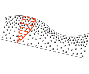
Figure 5. Evolution of a Poiseuille flow with an inlet height  $h_i$ to a fully developed particle-laden Nusselt flow for a system with bulk particle volume fraction $\phi _0 = 0.3$. The contour plot shows the particle volume fraction field; (a) $Pe_p = 1$, (b) $Pe_p = 10$.
4. Linear stability analysis
With the base state of the system and the route towards the fully developed base state evaluated in § 3 and 3.1, we now proceed to perform a linear stability analysis on the full system of (2.12)–(2.14). This is done by perturbing all the physical variables in the problem as a sum of their base states, and a sinusoidal wave of wavenumber  $k$ and wave speed $c$. Thus, each physical variable in the system (say $X$) is written in the form $X = X_b + \hat {X} \exp ({\textrm {i} k (x - c t)})$, with $X_b$ referring to the base flow variables and $\hat {X}$ referring to the infinitesimally small amplitude of the disturbances $(|\hat {X}|\ll |X_b|)$. We consider two-dimensional disturbances in the present study. The resulting equations after linearisation are
 $$\begin{gather} \{ {\rm i} k Re [ (u_b - c)(\mathcal{D}^2 - k^2) - u_b'' ] - 2 \kappa_b' (\mathcal{D}^2 - k^2) \mathcal{D} - \kappa_b (\mathcal{D}^2 - k^2)^2 - \kappa_b '' (\mathcal{D}^2 + k^2) \} \hat{\psi} \nonumber\\ = {\rm i} k \mathcal{D} \hat{N}_1 + (\mathcal{D}^2 + k^2) (\kappa_{b1} u_b' \hat{\phi}), \end{gather}$$
 $$\begin{gather}{\rm i} k \; \xi [ (u_b - c) \hat{\phi} - \phi_b' \hat{\psi} ] ={-}{\rm i} k \hat{J}_x - \mathcal{D} \hat{J}_y. \end{gather}$$
Here,  $\hat {\psi }$ and $\hat {\phi }$ are the perturbation streamfunction and particle volume fraction, respectively, $\mathcal {D}$ and primes denote the derivatives with respect to $y$ of the perturbation and base-state quantities, respectively, and $\kappa _{b1} = {\textrm {d}\kappa _b(\phi _b)}/{\textrm {d}\phi _b}$, with $\kappa _{b1}\hat {\phi }$ being equal to viscosity perturbation and $\hat {N}_1 = \hat {\varSigma }_{xx}^{NS} - \hat {\varSigma }_{yy}^{NS}$ corresponds to the normal stress difference perturbation. Subsequently, the linearised boundary conditions at $y = 1$ are
 $$\begin{gather} \left\{ \kappa_b \left( \mathcal{D}^2 + k^2 \right) - \left( {\rm i} k N_{b1} + 3 \right) \frac{1}{(c - u_b (1))} \right\} \hat{\psi} = 0, \end{gather}$$
 $$\begin{gather} \left\{ \kappa_b' (\mathcal{D}^2 + k^2) + \kappa_b (\mathcal{D}^2 - 3 k^2) \mathcal{D} + {\rm i} k Re (c - u_b(1)) \mathcal{D} \right. \nonumber\\ \left. {-}\left(3 \cot \alpha + k ^2 We \; Re \right) \frac{{\rm i} k}{(c- u_b(1))} \right\} \hat{\psi} + \mathcal{D} (\kappa_{b1} u_b' \hat{\phi}) + {\rm i} k \hat{N}_1 = 0, \end{gather}$$
 $$\begin{gather} - J_{xb} \frac{{\rm i} k }{(c - u_b(1))} \hat{\psi} + \hat{J}_y = 0, \end{gather}$$
and at  $y = 0$
 $$\begin{gather} \hat{\psi} = \mathcal{D} \hat{\psi} = 0, \end{gather}$$
 $$\begin{gather}\hat{J}_y = 0. \end{gather}$$
Here,  $N_{b1} = \varSigma _{b,xx}^{NS} - \varSigma _{b,yy}^{NS}$ is the base-state normal stress difference. The above system of modified Orr–Sommerfeld equations is similar to the corresponding system for a flow with viscosity stratification as first derived by Drazin (Reference Drazin1962) for a parallel flow and subsequently for free-surface flows by Craik & Smith (Reference Craik and Smith1968). However, the presence of additional terms arising from the particle-induced normal stress differences ( $N_{b1}, \hat {N}_1$) and particle flux terms ( $J_{xb}, \hat {J}_x, \hat {J}_y$) makes the above system of equations (4.1)–(4.7) unique. The terms arising from normal stress differences are absent while using the diffuse flux model as it does not account for the particle-induced normal stresses. Also, the term arising from the base-state normal stress difference, $\textrm {i} k N_{b1}$, in the boundary condition (4.3) is zero since the base-state normal stresses vanish at $y = 1$. In the interest of brevity, the expressions for perturbation particle fluxes ( $\hat {J}_x,\hat {J}_y$) and particle normal stresses ( $\hat {N}_1$) have been relegated to Appendix B.
4.1. Surface mode – long-wave instability
A gravity-driven liquid film on an inclined surface is unstable to long-wave disturbances (Benjamin Reference Benjamin1957; Yih Reference Yih1963). The linear and nonlinear regimes of the falling film instability for a Newtonian fluid have been studied extensively (Kalliadasis et al. Reference Kalliadasis, Ruyer-Quil, Scheid and Velarde2011). Taking cues from Yih (Reference Yih1963), we look for the surface mode of instability as one that is unstable at long wavelengths ( $k\ll 1$). For this, we pose expansions of the form $\psi =\psi _0+k \psi _1+\ldots$ and $c=c_0+k c_1+\ldots$. Subsequently, the leading-order equations become
 $$\begin{gather} \mathcal{D}^2 (\kappa_b \mathcal{D}^2 \hat{\psi}_0 + \kappa_{b1} u_b' \hat{\phi}_0 ) = 0, \end{gather}$$
 $$\begin{gather}\mathcal{D} \hat{J}_{y0} = 0, \end{gather}$$
with the boundary conditions at  $y = 1$
 $$\begin{gather} \left\{ \kappa_b \mathcal{D}^2 - \frac{3}{(c_0 - u_b (1))} \right\} \hat{\psi}_0 = 0, \end{gather}$$
 $$\begin{gather}\mathcal{D} (\kappa_b \mathcal{D}^2 \hat{\psi}_0 + \kappa_{b1} u_b' \hat{\phi}_0 ) = 0, \end{gather}$$
 $$\begin{gather}\hat{J}_{y0} = 0, \end{gather}$$
and at  $y = 0$
 $$\begin{gather} \hat{\psi}_0 = \mathcal{D} \hat{\psi}_0 = 0, \end{gather}$$
 $$\begin{gather}\hat{J}_{y0} = 0. \end{gather}$$
Solving for the above system, a dispersion relation can be obtained as
 \begin{equation} d_1 c_0^3 + d_2 c_0^2 + d_3 c_0 + d_4 = 0. \end{equation}
Here,  $d_1$, $d_2$, $d_3$ and $d_4$ are combinations of integrals that can be evaluated from the base-state solution. The expressions for evaluating the integrals in the above system are given in Appendix C. Equation (4.15) gives three roots, all of which are real. One of the roots corresponds to the surface mode; the one found by Yih (Reference Yih1963), albeit modified by the presence of particles (see figure 6). The other two modes are associated with the transport of the dispersed phase. This implies that we need to evaluate the system until ${O}(k)$ to obtain the growth rates, consistent with the behaviour known for the particle-free scenario. The ${O}(k)$ calculation of growth rate is algebraically tedious, involving several integrals that must be evaluated numerically. It is no more economical than an entire numerical computation. Such semi-analytical expressions for growth rates would also be dependent on the choice of constitutive model. We will instead focus on exploring why the presence of a microstructure should destabilise a falling film and then attempt to identify mechanisms that are not reliant on the choice of constitutive model.

Figure 6. Variation of the Doppler shifted wave speed,  $c_0-u_b(1)$, of the surface mode, plotted for a range of bulk particle volume fractions ( $\phi _0$) and Péclet numbers ( $Pe_p$) obtained from the long-wave dispersion relation – (4.15).
4.1.1. Mechanism of surface mode instability
In this section we discuss the mechanism of the surface instability, building on the insightful explanation of Smith (Reference Smith1990) for the falling film instability of a particle-free film. Consider perturbations to the system, leading to disturbances to the interface of the form  $\bar {h}(x,t) = h(x,t) - 1$. The base-state shear stress at the perturbed interface is non-zero, and can be written as $(\kappa _b u_b')' \bar {h}(x,t)$ acting along the flow direction (see figure 7a). Since the surface is a stress free zone, there must be a cancelling shear stress from the perturbations acting on the unperturbed surface. This compensatory shear stress now drives a flow that acts as the initial driving mechanism for the disturbance (see figure 7b). If we next consider the ${O}(k)$ equations, the $x-$momentum balance at this order is written as
 \begin{equation} \mathcal{D} (\kappa_b \mathcal{D} \hat{u}_1) = {\rm i}\, Re \; \hat{P}_0 - {\rm i}\, \hat{\varSigma}_{xx_0}^{NS} + Re [{\rm i} (u_b - c_0)\hat{u}_0 + u_b' \hat{v}_1] - \mathcal{D} (u_b' \kappa_{b1} \hat{\phi}_1). \end{equation}
Here, the leading-order equation  $(Re \; \hat {P}_0 - \hat {\varSigma }_{xx_0}^{NS} ) = - \hat {N}_{1_0} - \hat {\varSigma }_{b,yy}^{NS'} + 3 \cot {\alpha }$, is essentially the hydrostatic pressure term that acts to flatten the interface and drive a flow away from the crest. Inspecting the first inertial stress term, $\textrm {i} Re (u_b - c_0)\hat {u}_0$, it is obvious from the figure 8(a) that the sign of the term $(u_b - c_0)$ would determine whether this term would have a stabilising or a destabilising effect since the $\hat {u}_0$ is positive throughout the domain. For the surface mode, $u_b < c_0$ (see figure 6) throughout the domain as the disturbance tends to travel faster than the base-state fluid velocity. Thus the first inertial stress term has a destabilising effect. The second inertial term $\textrm {i} Re (-\textrm {i} u_b' \hat {v}_1)$ is also a negative term as $u_b'$ and $\textrm {i} \hat {v}_1$ are positive. Thus both the inertial stress terms contribute to the destabilisation of the system. The presence of the viscous term $\mathcal {D} (u_b' \kappa _{b1} \hat {\phi }_1)$ in (4.16) hints at the possibility of there being an instability even in the absence of fluid inertia. In § 4.2.1, we explore this and find the system to be unstable beyond a critical Péclet number.

Figure 7. Base-state shear stress developed on the perturbed interface – (a), leading to a leading-order perturbation flow in the film – (b). The dash lines indicate the unperturbed free surface.

Figure 8. Directions of the disturbance flow field generated by individual terms in the  ${O}(k)$ equations drawn in the reference frame moving with the phase velocity. (a) Denotes the inertial stress, (b) denotes the term arising due to the perturbative viscosity and (c) denotes the gravity.
Inhomogeneity in the particle concentration field could affect the dynamics in two ways: viscosity stratification in the base state and concentration perturbations in the momentum (4.16). To see how the variation in viscosity could affect stability, let us look at a reduced problem. Motivated by base-state profiles obtained in § 3, we consider a linearly viscosity stratified base state
 \begin{equation} \kappa_b=1+\epsilon(y-y_c). \end{equation}
We further simplify it by choosing the particle-free Nusselt flow as the unperturbed velocity field and assume the measure of stratification  $\epsilon \ll 1$. A long-wave analysis reveals the instability criterion to be
 \begin{equation} Re_c=\left\{\frac{5}{6}-\epsilon\frac{95}{64}\left(y_c-\frac{137}{399}\right)\right\}\left(\cot\alpha+\frac{k^2}{3Ca}\right)+{O}(\epsilon^2). \end{equation}
Our previous discussion of the  ${O}(k)$ flow field (see schematic in figure 8) has highlighted the destabilising roles of different terms on the right-hand side of (4.16). Thus the viscosity stratification, particle induced in the present problem due to shear-induced migration, destabilises the system further depending on location in the film ( $y_c$) where the particle concentration exceeds its bulk value. The base-state concentration profiles discussed in § 3 (also see figure 2b,d) have a $y_c\approx 0.5$, indicating a likelihood of enhanced instability as per the reduced model discussed above.
The reduced model is a one-way coupled system with the assumption of a particle-free Nusselt base-state flow. The base-state flow consistent with the linear viscosity stratification would provide a numerical estimate of the critical Reynolds number (4.18) as a function of  $\epsilon$ and $y_c$, but the conclusions remain unchanged. The complete two-way coupled system (4.1)–(4.7) would continue to exhibit the enhanced stability characteristics, which we will discuss further in the next section using finite wavenumber analysis. The current system has an interesting analogy with the stability of film flow down heated or cooled inclined plates. Most studies on the role of thermal forces on the stability of falling film focus on thermocapillary effects, ignoring thermal effects in the bulk (Kalliadasis et al. Reference Kalliadasis, Ruyer-Quil, Scheid and Velarde2011). The study by Craik & Smith (Reference Craik and Smith1968) and then by Goussis & Kelly (Reference Goussis and Kelly1985) examined the role of viscosity stratification on the stability of a falling film. Goussis & Kelly (Reference Goussis and Kelly1985) motivated viscosity stratification as a consequence of a heated or cooled substrate and thus removed the restriction in the study of Craik & Smith (Reference Craik and Smith1968), of viscosity being purely convected by the flow. They observed that the instability threshold gets lowered when the viscosity gradients are directed towards the free surface (heated plate). This behaviour is consistent with observations in the current study, although the underlying physics behind a viscosity stratification directed towards the interface is a different one – shear-induced migration.
4.2. Finite wavenumber analysis
In the previous section, we discussed the mechanism of the surface instability using a long-wave theory. We will now probe the system's stability to disturbances of arbitrary wavelengths, analysing the modification of the surface instability and the possibility of any additional instabilities. The subsequent paragraphs provide a detailed account of particles’ effect on the system's stability. We show the presence of two modes of instability – a surface mode described in the previous section and a shear mode instability and discuss the destabilising role of particles on both modes of instability. A key takeaway from this section is the plot of neutral stability curves (see figure 12), depicting the existence of the two unstable modes in the  $Re-k$ plane for combinations of $\phi _0$ and $Pe_p$. Subsequently, we present the results of specific cases to understand the source of destabilisation. The ‘unstable’ viscosity stratification set up by the shear-induced migration of particles plays the most dominant role in enhancing the instability. Notably, we also demonstrate the independence of this enhanced instability on the choice of constitutive model. The previous section also showed that the destabilisation mechanism due to viscosity perturbations does not depend on fluid inertia. Therefore, in § 4.2.1, we probe the possibility of this instability persisting in the limit of $Re=0$. In the inertialess limit, we find that the surface mode does get destabilised beyond a critical $Pe_p$, for a fixed $\phi _0$.
To study the stability of the system subjected to disturbances of arbitrary wavelengths, we solve the system of linear equations (4.1)–(4.7) by framing it as an eigenvalue problem, with  $c$ as the eigenvalue. This eigenvalue problem is solved numerically using the Chebyshev spectral collocation method (Trefethen Reference Trefethen2000). With the spatial discretisation done on a Chebyshev domain, we use MATLAB to solve the resulting linear equations forming the eigenvalue problem. To gain confidence in our numerical solver, we validate it with the results by Floryan et al. (Reference Floryan, Davis and Kelly1987) for instabilities in a particle-free falling film, over a range of Reynolds numbers and wavenumbers. The comparisons thus made are listed in table 2. We begin by looking at the surface mode instability using the model by Frank et al. (Reference Frank, Anderson, Weeks and Morris2003) to describe the particle phase. Figure 9 shows plots of the growth rate ( $c_i$) of the surface mode compared between $Pe_p = 0.1$ and $1$. The two curves are indistinguishable for a bulk particle volume fraction of $\phi _0 = 0.1$. However, when we increase the bulk particle volume fraction, $\phi _0 = 0.3$, $Pe_p = 1$ can be seen to predict a higher growth rate. This trend of increasing Péclet number leading to increased growth rate follows as seen in the plot of maximum growth rates obtained for a range of Péclet numbers in figure 10(a). We also track the wavenumber corresponding to the maximum growth rates – $k_{{max}}$. We observe that, with increasing $Pe_p$, the maximum growth rate is attained for progressively longer waves for the case with a higher bulk particle volume fraction ( $\phi _0 = 0.3$). However, for $\phi _0 = 0.1$, there is no perceptible change in the wavenumber at which the maximum growth rate occurs.
Table 1. Estimates of physical parameters in a particle-laden falling film.

Table 2. Comparisons for validation of the stability code with the results by Floryan et al. (Reference Floryan, Davis and Kelly1987) for  $\alpha = 1^0$.


Figure 9. Comparisons of the imaginary part of the wave speed corresponding to the surface mode for (a)  $\phi _0 = 0.1$ and (b) $\phi _0 = 0.3$; $Pe_p = 0.1$ (- - -); $Pe_p = 1$ (—) over a range of wavenumbers ( $k$) with $Re = 20$.

Figure 10. Plots of the maximum growth rate –  $c_i^{max}$ (a) and the wavenumber at which the maximum growth rate occurs – $k_{max}$ (b) for the surface mode over a range of $Pe_p$ for $\phi _0 = 0.3$ (blue lines) and $\phi _0 = 0.1$ (black lines) with $Re = 20$.
The long-wave surface instability is not the only mode of destabilisation for a falling film. The background velocity profile, a parabolic Nusselt flow in the particle-free case, admits a viscous Tollmien–Schlichting shear instability similar to those found in plane Poiseuille and Blasius boundary layer flows (Drazin & Reid Reference Drazin and Reid2004). The shear mode is a short-wave instability that occurs at a large Reynolds number, not involving any interfacial disturbances. For the shear mode, viscous effects play a dual role. They do the expected stabilisation of the flow via viscous dissipation, but they also introduce a phase shift between the streamwise and wall-normal velocity disturbances due to viscous effects in the critical layer (the location where the flow speed matches the wave speed). This phase shift is responsible for a non-zero Reynolds stress and creates a possibility for the growth of disturbance kinetic energy. Since the two viscous effects compete against each other, the shear mode for a falling film is expected to manifest at a large Reynolds number. We plot the vorticity fields corresponding to the surface mode and shear mode in figure 11. The structures of the eigenfunctions are distinctly different, with the shear mode exhibiting a localised peak near the bottom substrate as previously noted by Chin et al. (Reference Chin, Abernath and Bertschy1986). The wall-normal coordinate for the shear mode is scaled with  $(kRe)^{1/3}$, consistent with critical layer arguments (Maslowe Reference Maslowe1986). Floryan et al. (Reference Floryan, Davis and Kelly1987) analysed the dynamics of the two modes in a falling film and observed that the shear mode could prevail over the surface mode only the inclination angle is very small.

Figure 11. Vorticity fields for the surface mode (a) and shear mode (b) at  $t = 0.001$ for the case of $\phi _b = 0.3$ and $Pe_p = 1$: (a) $k=0.01$, $Re = 20$; (b) $k=0.5$, $Re = 10^6$.

Figure 12. Neutral stability curves corresponding to the surface mode (a) and the shear mode (b), for  $\phi _0 = 0.3$ (blue), $\phi _0 = 0.1$ (black); $Pe_p = 0.1$ (- - -), $Pe_p = 1$ (—).
To see the role of bulk volume fraction and Péclet number in the instability thresholds of both the surface and shear mode instabilities, we plot neutral curves for both the modes of instability in the Reynolds number–wavenumber plane. For a fixed  $Pe_p$, we anticipate that an increase in bulk particle volume fraction leading to an increase in suspension viscosity would have a stabilising effect. The novel result in the present study is the role non-Brownian effects play for fixed $\phi _0$ but varying $Pe_p$. Figure 12 shows that the surface mode instability threshold is lowered when the value of $Pe_p$ is increased from 0.1 to 1. For $Pe_p = 1$, the instability threshold is lowered even below the instability threshold for a film devoid of particles! The enhanced instabilities due to the dispersed phase are present for both the surface and shear modes of instability. Why should the underlying microstructure destabilise a falling film further? We have partially answered this query in our discussion of the long-wave surface mode of a one-way coupled reduced model via a ‘unstable’ viscosity stratification that naturally arises due to shear-induced migration. The two-way coupled full model has additional terms, and it is not apparent what plays the role of the leading destabilising actor. Moreover, we also wish to include the shear mode of instability in our attempt, excluded earlier in the long-wave discussion.
To answer the above question, we revisit the modified Orr–Sommerfeld equation (4.1). In comparison with the Orr–Sommerfeld equation corresponding to a system devoid of any particles, we find additional terms arising from the first and second derivatives of the base-state viscosity ( $\kappa _b'$ and $\kappa _b''$), a term arising from the perturbation of viscosity ( $\mathcal {D}^2 (\kappa _{b1} u_b' \hat {\phi })$) and a term involving the gradient to the perturbation normal stress difference ( $\mathcal {D}\hat {N}_1$). To see how these additional terms contribute to the enhancement of instability, we run three model cases listed in table 3. With case 1, we have a problem that accounts only for the base-state particle volume fraction dependent viscosity gradients – a one-way coupled problem. Case 2 is one where we switch off the derivatives of the base-state viscosity alone. Finally, case 3 is when the derivatives of the base-state viscosity and the perturbative viscosity term ( $\kappa _{b1}$) are all switched off. Figure 13(a) shows the neutral stability curve of the surface mode instability corresponding to these special conditions for a bulk particle volume fraction of $\phi _0 = 0.3$. The most obvious conclusion is that the viscosity perturbation term makes the largest contribution as it single handedly pushes the threshold of instability below that of an analogous clear film. However, the term arising from the normal stress difference does not have any noticeable impact on the instability threshold. Comparing case 1 and case 2, we see that the derivatives of the base-state viscosity, representative of viscosity stratification, play second fiddle in the instability.

Figure 13. Neutral stability curves corresponding to the surface mode (a) and the shear mode (b), for  $\phi _0 = 0.3$ (blue lines), $Pe_p = 0.1$ (- - -) and $Pe_p = 1$ (—) . The red lines correspond to the special cases – case 1 (—), case 2 (- - -) and case 3 ( $\cdots$) listed in table 3 for $\phi _0 = 0.3$ and $Pe_p = 1$ with all other parameters being the same.
Table 3. Cases run to identify the destabilising terms.

Unlike the surface mode that is unstable over long wavelengths, the shear mode is unstable over shorter wavelengths and large Reynolds numbers. Looking at figure 12(b), we see that increasing bulk volume fraction invariably leads to increasing the instability threshold. However, we still see that, with Péclet number  $Pe_p = 1$, the instability threshold does lower for a given bulk particle volume fraction. Looking at the results of the model cases (see figure 13b), we again note that the derivatives of the base-state viscosity play a secondary role in the enhancement of instability here. Wazzan, Okamura & Smith (Reference Wazzan, Okamura and Smith1968) has previously shown this enhancement of instability arising from the derivatives of the base-state viscosity in the context of Tollmien–Schlichting disturbances on a flow over a heated plate. Typically, the studies on wall-bounded viscosity stratified flows indicate that, when viscosity increases along the gradient direction away from the wall, the system gets stabilised (Wall & Wilson Reference Wall and Wilson1996; Sameen & Govindarajan Reference Sameen and Govindarajan2007). This is due to the velocity profile becoming fuller with such a viscosity stratification (Sameen & Govindarajan Reference Sameen and Govindarajan2007). Also, a viscosity stratification that decreases along the gradient direction away from the wall is in turn known to have a destabilising effect (Sameen & Govindarajan Reference Sameen and Govindarajan2007). Moreover, Ranganathan & Govindarajan (Reference Ranganathan and Govindarajan2001) (see also Govindarajan Reference Govindarajan2004) found that the location of the viscosity stratification relative to the critical layer can have a stabilising/destabilising effect on the system. However, particle migration leads to lowering of the viscosity below the viscosity corresponding to the bulk particle volume fraction near the bottom wall and higher than the same near the free surface. This in turn leads to the velocity profiles becoming less full in the region towards the wall and blunt near the free surface, leading to a destabilising role in the system. Also, as seen with the surface mode, the viscosity perturbation term has the most significant role in enhancing the instability.
A valid criticism of linear stability studies involving any complex fluid, flowing suspensions being an example, is to what extent the reported instabilities stem from realistic physics? There is a possibility that the instabilities are due to the choice of the constitutive model, arising due to the linearisation of empirical relations. Here we have attempted to discuss mechanisms for the enhanced instabilities in a particle-laden falling film that are agnostic of the choice of the constitutive model. To investigate further how the choice of constitutive model can alter the predictions of the instability threshold, we next compare the neutral curves predicted while using the model by Frank et al. (Reference Frank, Anderson, Weeks and Morris2003) with the predictions of the diffuse flux model (see figure 14). We find that, for the case of  $Pe_p = 0.1$, the instability threshold predictions corresponding to both the surface and shear modes are indistinguishable between the two models. However, the diffuse flux model underpredicts the instability threshold for the surface and shear instability mode for $Pe_p = 1$. This behaviour can be reasoned by looking at the base-state comparisons between the two models (see figure 2). It is immediately apparent that the corresponding magnitude of the derivatives of base-state viscosity is lower for the diffuse flux model in comparison with the model by Frank et al. (Reference Frank, Anderson, Weeks and Morris2003). Since this magnitude directly contributes to destabilising the flow, the instability threshold also gets underpredicted. It is, however, possible to push the instability thresholds from the diffuse flux model closer to the predictions of the model by Frank et al. (Reference Frank, Anderson, Weeks and Morris2003) by altering the values of the constants $K_c$ and $K_v$. The arbitrariness can be eliminated if the values of $K_c$ and $K_v$ are determined from experimentally determined velocity and concentration profiles of a falling film suspension flow. However, the observation that the inclusion of particles with their associated Péclet number at $Pe_p = 1$ does push the instability threshold below that of even a clear film continues to be correct. Also, the enhancement of instability of the shear mode for a given bulk volume fraction remains faithful between the predictions of the two models.

Figure 14. Neutral stability curves corresponding to the surface mode (a) and the shear mode (b), with comparisons between the suspension balance based model by Frank et al. (Reference Frank, Anderson, Weeks and Morris2003) (blue lines) and the diffuse flux model by Phillips et al. (Reference Phillips, Armstrong, Brown, Graham and Abbott1992) (red lines) for  $\phi _0 = 0.3$, $Pe_p = 0.1$ (- - -) and $Pe_p = 1$ (—).
Having compared a suspension balance based model and the diffuse flux model, we make one last check of consistency by comparing the results with the predictions obtained using the theoretical model of Brady & Vicic (Reference Brady and Vicic1995) – one that is valid for dilute particle volume fractions and small Péclet numbers (2.21a,b). Figure 15 shows comparisons between the model by Brady & Vicic (Reference Brady and Vicic1995) and the model by Frank et al. (Reference Frank, Anderson, Weeks and Morris2003) for a bulk volume fraction of  $\phi _0 = 0.1$. Here again, our observations regarding the enhancement of instability remain consistent for both the surface and shear mode. However, the threshold of instability is uniformly lowered for both values of Péclet number ( $Pe_p = 0.1$ and 1) in comparison with the prediction when using the model by Frank et al. (Reference Frank, Anderson, Weeks and Morris2003). This behaviour can be attributed to the choice of the particle volume fraction dependent viscosity, as the analytical expression underpredicts the viscosity compared with the Krieger–Dougherty correlation. A similar linear stability analysis can also be performed using any of the other particle migration models listed in Appendix A.

Figure 15. Neutral stability curves corresponding to the surface mode (a) and the shear mode (b), with comparisons between the suspension balance based model by Frank et al. (Reference Frank, Anderson, Weeks and Morris2003) (black lines) and the analytical model by Brady & Vicic (Reference Brady and Vicic1995) (red lines) for  $\phi _0 = 0.1$, $Pe_p = 0.1$ (- - -) and $Pe_p = 1$ (—).
4.2.1. Limit of zero fluid inertia
Thus far, we have studied the role of particles on the surface mode as a modulator acting on top of the destabilising fluid inertia. However, the destabilising viscosity stratification set up by the particles is independent of fluid inertia. Therefore, it is now appropriate to ask if the presence of particles can solely act to destabilise the system without the aid of fluid inertia. To study this, we take the limit of  $Re = 0$ in the linearised equations (4.1)–(4.7). It must be noted that, to retain the surface tension term at $Re = 0$, we replace $We \, Re$ with $Ca^{-1}$ in (4.4). The subsequent calculations are done with a capillary number $Ca = 10^{-3}$.
Figure 16(a) shows the maximum growth rate achieved by the surface mode for a range of Péclet numbers. The trend of increasing Péclet numbers leading to increased growth rates observed in the finite fluid inertia case (dashed lines in figure 16a) remains true with the absence of fluid inertia as well. Comparing the growth rates obtained both with and without fluid inertia, we observe that shear-induced migration and fluid inertia complement each other in enhancing the instability. We also track the wavenumber corresponding to the maximum growth rate –  $k_{max}$. As expected, we find the need for the longest waves near the vicinity of the critical Péclet number. After this, $k_{max}$ goes on to increase and subsequently decrease. Therefore, for higher Péclet numbers, there is a need for progressively longer waves to achieve the highest growth rates. This again remains consistent with the observations made in the finite fluid inertia case (dashed lines in figure 16b). To further ascertain the instability, we plot the neutral curves in the wavenumber–Péclet number plane (figure 17). Unlike the finite fluid inertia case, we find that the envelope of the unstable region is larger for the higher particle volume fraction $\phi _0 = 0.3$ than with $\phi _0 = 0.1$. This can be attributed to the particle volume fraction being the sole destabilising agent in this system. Also, we observe that the threshold of instability is lowered for the higher particle volume fraction.

Figure 16. Plots of the maximum growth rate –  $c_i^{max}$ (a) and the wavenumber at which the maximum growth rate occurs – $k_{max}$ (b) for the surface mode over a range of $Pe_p$ for $\phi _0 = 0.3$ (blue lines) with $Re = 0$. Dashed lines denote the case of $Re = 20$.

Figure 17. Neutral stability curves corresponding to the surface mode in the  $k_c\text{--} Pe_p$ plane for $\phi _0 = 0.3$ (blue), $\phi _0 = 0.1$ (black) for $Re = 0$.
5. Discussion and conclusions
We have explored the role of particles and the normal stresses they exert on the stability of a particle-laden, gravity-driven, shallow flow down an incline. The particles studied were of a specific size range such that the particle-induced normal stresses have a combination of thermal and athermal contributions. A conservation equation describes the evolution of the particle phase with the particle fluxes described either by a suspension balance based model or the diffuse flux model. The fluid experiences the role of the particulate phase through the modification of the viscosity and the additional stresses contributed by the particles. The choice of the exact form of these fluxes, stresses and particle volume fraction dependent viscosity would depend on the specific choice of constitutive model. We first explored the effect of the choice of constitutive model – the suspension balance model and diffuse flux model – and Péclet number ( $Pe_p$) on the steady and unidirectional base-state solution of a flat film flow. Nott, Guazzelli & Pouliquen (Reference Nott, Guazzelli and Pouliquen2011) found that the form of suspension balance model as written by Nott & Brady (Reference Nott and Brady1994) (see (2.10)) is inadequate. However, we used an empirical version of the suspension model proposed by Frank et al. (Reference Frank, Anderson, Weeks and Morris2003) in our calculations. Therefore, as noted by Nott et al. (Reference Nott, Guazzelli and Pouliquen2011), the particle phase stress could have been captured by the phenomenological form chosen for $\boldsymbol {\varSigma }^p$. Nevertheless, it will be evident in further discussions that this choice of constitutive model does not influence the nature of instability. Independent of the choice of constitutive model, we observed that smaller Péclet numbers led to an almost uniform distribution of particles as Brownian diffusion became dominant. However, increasing values of $Pe_p$ led to increased accumulation of particles at the free surface. This accumulation was due to the interface being stress free. The fluxes indicated that particles migrated towards zones of low stresses, hence the accumulation at the stress-free surface.
After studying the fully developed base state, we investigated the route towards the fully developed state if one were to start from a Poiseuille flow with uniform particle distribution. We did this under the boundary layer approximation to obtain the velocity field, particle volume fraction field and the free interface. Previous studies have experimentally and theoretically studied this development in the context of particle-laden pressure-driven flows, without a free interface (Hampton et al. Reference Hampton, Mammoli, Graham, Tetlow and Altobelli1997; Miller & Morris Reference Miller and Morris2006; Semwogerere et al. Reference Semwogerere, Morris and Weeks2007). We found that the entrance lengths decrease with increasing bulk particle volume fractions. A similar reduction in entrance lengths on a particle-laden pressure-driven flow inside a circular conduit was first observed in experiments by Hampton et al. (Reference Hampton, Mammoli, Graham, Tetlow and Altobelli1997). We also found that increasing Péclet number led to an increase in the entrance length. This observation was consistent with the experimental and theoretical calculations of Semwogerere et al. (Reference Semwogerere, Morris and Weeks2007) for a particle-laden pressure-driven flow with rigid top and bottom boundaries. Thus, we found that the thermal contribution to the particle-induced normal stresses makes a huge contribution in the development towards a fully developed state, a point previously noted by Semwogerere et al. (Reference Semwogerere, Morris and Weeks2007).
To study the effect of these particles on the system's stability, we then performed a linear stability analysis over the previously obtained base states. For small values of Péclet number, increasing bulk particle volume fractions led to an increase in the threshold of instability for both modes of instability, thus having a stabilising effect. This can be attributed to the particles’ almost uniform distribution, leading to a uniform increase in viscosity throughout the domain. We also found that, for a Péclet number of  $Pe_p = 1$, the instability threshold decreased for a given bulk particle concentration for both the shear and surface modes. This was due to the increase in the magnitude of the gradients of the base viscosity and the presence of the perturbative viscosity term as shown in § 4.2 and in the stability calculations on the problem of a flow overheated/cooled plates by Wazzan et al. (Reference Wazzan, Okamura and Smith1968). However, we also found that the instability threshold gets lowered beyond the case of a system devoid of particles for the surface mode of instability. The terms mentioned above were again found to be responsible for this enhanced instability of the surface mode. This remains consistent with the findings of Goussis & Kelly (Reference Goussis and Kelly1985) who studied the effects of viscosity stratification arising from heating/cooling the bottom substrate.
Finally, to see how the choice of constitutive model for the particle phase can influence the predictions of instability thresholds, we compared the predictions obtained using three models – the suspension balance based model by Frank et al. (Reference Frank, Anderson, Weeks and Morris2003), the phenomenological model by Phillips et al. (Reference Phillips, Armstrong, Brown, Graham and Abbott1992) and the analytical model by Brady & Vicic (Reference Brady and Vicic1995). While the exact values of the instability thresholds predicted varied between the three and were also largely dependent on the empirical constants associated with each of these models, we found that the observation that an increase in Péclet number led to an enhancement of the instability remained consistent across the three models. This showed that the predictions of the enhanced instability were a direct consequence of shear-induced migration of particles and not an artefact of the choice of model as long as the chosen model accounted for shear-induced migration.
With the destabilising role of particles in the system well established, we then explored the possibility of instability triggered purely by the presence of particles. This was done by taking the limit of  $Re = 0$, thereby removing the destabilising fluid inertia. A similar linear stability analysis on the resulting system revealed the presence of an unstable surface mode beyond a critical Péclet number. We found that increased particle volume fractions decreased the stability threshold. The findings of the presence of instability even with the absence of fluid inertia and an increased destabilisation of the system with increasing particle volume fractions is consistent with the experimental observations of Timberlake & Morris (Reference Timberlake and Morris2005) performed for highly viscous flows ( $Re < 0.01$). They observe higher surface corrugations with increasing bulk particle volume fractions, albeit for higher Péclet numbers. This is attributed to the particle volume fraction being the sole destabilising agent in the system with the lack of fluid inertia. It must be noted that, in this limit, there is no possibility of a shear mode instability as it is exclusive to high Reynolds numbers.
After discussing the instability in detail, it is now worth attempting to quantify the role of particles in terms of physical parameters. An interesting question here would be to ask the difference in the wavelength of disturbance required to trigger the surface mode instability between two liquids of comparable bulk viscosity – one laden with particles and the other devoid of particles. Suppose we consider an experimental set-up with the following physical parameters –  $a = 0.04\,\mathrm {\mu }\textrm {m}$, $\rho = 1000\,\textrm {kg}\,\textrm {m}^{-3}$, $g = 9.81\,\textrm {m}\,\textrm {s}^{-2}$, $h_0 = 10^{-2}\,\textrm {m}$, $\mu _f = 0.46\,\textrm {kg}\,\textrm {m}^{-1}\,\textrm {s}^{-1}$ and $\alpha = 45^{\circ }$. For the system devoid of particles, these parameters would correspond to a Reynolds number in the vicinity of the criticality condition. We predict that a disturbance with wavelength $\gtrapprox 7.5\,\textrm {m}$ is required to trigger the instability. But for the corresponding system with particles (here $Pe_p \approx 6.7$), we predict the critical wavelength required to be $\gtrapprox 1.1\,\textrm {m}$. With increasing fluid inertia, we predict that the critical wavelength is almost the same between the two systems (see figure 12).
Surface corrugations arising due to shear-induced migration of particles in free-surface flows have been experimentally observed in the context of shear flows (Tirumkudulu, Tripathi & Acrivos Reference Tirumkudulu, Tripathi and Acrivos1999; Loimer, Nir & Semiat Reference Loimer, Nir and Semiat2002), gravity-driven film flows (Timberlake & Morris Reference Timberlake and Morris2005) and open channel flows (Singh, Nir & Semiat Reference Singh, Nir and Semiat2006; Kumar et al. Reference Kumar, Medhi and Singh2016). Our predictions of an enhanced instability of the surface mode remained consistent with the experimental observations by Timberlake & Morris (Reference Timberlake and Morris2005). Although they study particle suspensions with Péclet numbers that are significantly larger, the experiments showed surface deformations happening in a highly viscous slow flow down an incline with  $Re \ll 1$. The occurrence of larger surface corrugations with suspensions of larger particles reported by Kumar et al. (Reference Kumar, Medhi and Singh2016) can also be related to our predictions of higher growth rates for increasing Péclet number. However, our analyses were limited to infinitesimal disturbances and dealt with the waves’ inception, whereas the experimental observations showed highly nonlinear wave formations. To be able to better relate to the experimental observations, future work could involve studying the nonlinear regime of particle-laden free-surface flows.
We have specifically refrained from accessing higher particle volume fractions and Péclet numbers in our calculations, both of which could lead to a jammed state at the interface. Accumulation of particles at the free interface can lead to the interface behaving like an elastic solid (Dixit & Homsy Reference Dixit and Homsy2013a) and also alter the surface tension (Dixit & Homsy Reference Dixit and Homsy2013b). Another aspect that becomes important is the glass transition that typically occurs at volume fraction  $\approx 0.59$ (Ikeda, Berthier & Sollich Reference Ikeda, Berthier and Sollich2012). These additional physics are safely ignored in the current study as we choose smaller particle concentrations and lower Péclet numbers. However, accommodating higher particle concentrations and Péclet numbers would entail using a concentration dependent surface tension and surface viscosity (Hu, Fu & Yang Reference Hu, Fu and Yang2020) with the inclusion of Marangoni effects, and using constitutive models for the particle phase that incorporate the physics of glass and jamming transitions (Ikeda et al. Reference Ikeda, Berthier and Sollich2012; Ikeda, Berthier & Sollich Reference Ikeda, Berthier and Sollich2013).
In the current study, we have focused solely on the role of neutrally buoyant particles on the stability of a gravity-driven shallow flow. However, flows occurring in both natural and engineering scenarios could be laden with non-neutrally buoyant particles, with non-negligible particle inertia. Modelling sediment transport in free-surface flows is one such scenario that continues to be a challenging multiphase problem (Ouda & Toorman Reference Ouda and Toorman2019). In the inertialess regime, the presence of negatively buoyant particles can lead to the creation of an unstable density profile arising due to particle migration in the flow, as shown previously by Carpen & Brady (Reference Carpen and Brady2002) in the context of fluid flow in an inclined channel with rigid boundaries. In their study, particle migration led to an accumulation of particles in the centre of the channel. An interesting future direction could involve understanding what would happen to the stability of a gravity-driven free-surface flow when laden with negatively buoyant particles. The presence of a free surface could create an unstable density profile that is set up due to the competition between shear-induced migration, which would encourage particles to migrate towards the free surface, and the buoyancy forces.
Acknowledgements
The authors acknowledge support from IIT Madras for its support of the ‘Geophysical Flows Lab’ research initiative under the Institute of Eminence framework.
Declaration of interests
The authors report no conflict of interest.
Appendix A. Base-state comparisons of various particle migration models
We discuss some of the particle migration models mentioned in the literature. Table 4 lists the models to be discussed and the corresponding equations. We first have the diffuse flux model – a phenomenological model formulated by Phillips et al. (Reference Phillips, Armstrong, Brown, Graham and Abbott1992). This model can accommodate particles with arbitrary Péclet numbers due to the inclusion of the Brownian diffusion term. We then have the suspension balance model, first derived by Nott & Brady (Reference Nott and Brady1994) exclusively for particles with  $Pe_p \rightarrow \infty$, and later extended to accommodate the presence of particle-induced normal stress differences using functional arguments by Morris & Boulay (Reference Morris and Boulay1999), and using empirical relations by Zarraga et al. (Reference Zarraga, Hill and Leighton2000). Miller & Morris (Reference Miller and Morris2006) included a non-local shear stress term to avoid the unphysical blow-up of particle volume fraction at zones of zero shear rate. Frank et al. (Reference Frank, Anderson, Weeks and Morris2003) wrote down the relation for the particle-induced normal stress with a combination of thermal and athermal stress contributions, making it valid for particles with arbitrary Péclet numbers. However, all of the previously mentioned models did not account for the shear-thinning aspect of these suspensions. Buyevich & Kapbsov (Reference Buyevich and Kapbsov1999) on the other hand, wrote down expressions for the shear viscosity while accounting for shear-thinning and particle-induced normal stresses with contributions from both thermal and athermal effects.
To compare the predictions of these models when applied to calculating the base state of a gravity-driven falling film, we solve the (3.1) and (3.3) with the boundary conditions (3.4) and (3.5). Figure 18 shows the base-state comparisons between the diffuse flux model, the suspension balance based models by Nott & Brady (Reference Nott and Brady1994) and Miller & Morris (Reference Miller and Morris2006) and the model by Buyevich & Kapbsov (Reference Buyevich and Kapbsov1999) (solved at the  $Pe_p \rightarrow \infty$ limit). For $\phi _0 = 0.01$, the velocity profiles vary minimally between the different models. However, there is a significant difference between the predictions of the particle volume fraction profiles, even for this low bulk volume fraction. For increasing bulk concentration, all models except for the model by Miller & Morris (Reference Miller and Morris2006) predict that the particle volume fraction reaches maximum packing fraction at the free interface. This is attributed to the inclusion of the non-local shear stress term. Figure 19 shows the comparisons of the velocity and particle concentration profile predictions between models exclusively based on the suspension balance approach – Nott & Brady (Reference Nott and Brady1994), Zarraga et al. (Reference Zarraga, Hill and Leighton2000), Morris & Boulay (Reference Morris and Boulay1999) and Miller & Morris (Reference Miller and Morris2006).

Figure 18. Comparison of base states obtained using the models by Phillips et al. (Reference Phillips, Armstrong, Brown, Graham and Abbott1992) – diffuse flux model (magenta lines), Buyevich & Kapbsov (Reference Buyevich and Kapbsov1999) (cyan lines), Nott & Brady (Reference Nott and Brady1994) (green lines), Miller & Morris (Reference Miller and Morris2006) with  $a_s = 0.1$ (grey lines) and with $a_s = 0.01$ (black lines) for bulk particle volume fractions $\phi _0 = 0.01$ (a,b), $\phi _0 = 0.3$ (c,d) and $\phi _0 = 0.5$ (e, f).
Table 4. For caption see next page.


Figure 19. Comparison of base states obtained using the models by Zarraga et al. (Reference Zarraga, Hill and Leighton2000) (red lines), Nott & Brady (Reference Nott and Brady1994) (green lines), Morris & Boulay (Reference Morris and Boulay1999) (blue lines), Miller & Morris (Reference Miller and Morris2006) with  $a_s = 0.1$ (grey lines) and with $a_s = 0.001$ (black lines) for bulk particle volume fractions $\phi _0 = 0.01$ (a,b), $\phi _0 = 0.3$ (c,d) and $\phi _0 = 0.5$ (e, f).
Appendix B. Linearised expressions corresponding to the models in consideration
Table 5. For caption see next page.

Appendix C. Expressions for the long-wave analysis
The expressions for solving the dispersion relation in (4.15) are
 $$\begin{gather} d_1 = \xi J_4, \end{gather}$$
 $$\begin{gather} d_2 ={-} L_2 + \xi \left( J_2 - J_3 + 9 I_2 J_6 - J_4 (3 I_1 + 9 I_3 + 2 u_b(1)) \right), \end{gather}$$
 $$\begin{gather} d_3 ={-} 3 I_2 (J_{xb}(1) + 3 L_1) + 3 I_1 L_2 + 9 I_3 L_2 + 2 L_2 u_b(1) \nonumber\\ + \xi \left[ - 3 (I_1 + 3 I_3) (J_2 - J_3) + ({-}2 J_2 + 2 J_3 + 3 I_1 J_4 + 9 I_3 J_4) u_b(1) \right. \nonumber\\ \left. + J_4 u_b(1)^2 + 9 I_2 (J_1 - J_5 - J_6 u_b(1)) \right], \\ d_4 = 3 I_2 (J_{xb}(1) + 3 L_1) u_b(1) - L_2 u_b(1) (3I_1 + 9 I_3 + u_b(1)) \nonumber\\+ \xi \left[ u_b(1) (9 I_2 (J_5 - J_1) + (J_2 - J_3) (3 I_1 + 9 I_3 + u_b(1)) ) \right]. \end{gather}$$
At  ${O}(1)$, the particle-induced stress can be written as $\varSigma _{yy0} = \mathcal {F}_y(\phi _b) \phi _0 + \mathcal {G}_y(\phi _b) \mathcal {D}^2 \psi _0$. With this, the relevant expressions are listed below
 $$\begin{gather} r_1 = (\mathcal{F}_y + 3 \mathcal{G}_y \kappa_{b1} \kappa_b^{{-}2} (y-1))^{{-}1}, \end{gather}$$
 $$\begin{gather}r_2 ={-} \mathcal{G}_y \kappa_b^{{-}1} r_1, \end{gather}$$
 $$\begin{gather}J_1 = \int_0^1 \phi_b' \int_0^y \int_0^{y'} \left[ \kappa_b^{{-}1} + 3 \kappa_{b1} \kappa_b^{{-}2} (y-1) r_2 \right]\,{{\rm d}y}\,{{\rm d}y}'\,{{\rm d} y}'', \end{gather}$$
 $$\begin{gather}J_2 = \int_0^1 \phi_b' \int_0^y \int_0^{y'} \left[ 3 \kappa_{b1} \kappa_b^{{-}2} (y-1) r_1 \right]\,{{\rm d} y}\,{{\rm d} y}'\,{{\rm d}y}'', \end{gather}$$
 $$\begin{gather}J_3 = \int_0^1 u_b r_1\,{{\rm d}y}, \end{gather}$$
 $$\begin{gather}J_4 = \int_0^1 r_1 \,{{\rm d} y}, \end{gather}$$
 $$\begin{gather}J_5 = \int_0^1 u_b r_2\,{{\rm d} y}, \end{gather}$$
 $$\begin{gather}J_6 = \int_0^1 r_2 \,{{\rm d} y}, \end{gather}$$
 $$\begin{gather}I_1 = \int_0^1 \int_0^y \kappa_b^{{-}1}\,{{\rm d} y}\,{{\rm d} y}', \end{gather}$$
 $$\begin{gather}I_2 = \int_0^1 \int_0^y \kappa_{b1} \kappa_b^{{-}2} (y-1) r1 \,{{\rm d} y}\, {{\rm d} y}', \end{gather}$$
 $$\begin{gather}I_3 = \int_0^1 \int_0^y \kappa_{b1} \kappa_b^{{-}2} (y-1) r2 \,{{\rm d} y}\,{{\rm d} y}', \end{gather}$$
 $$\begin{gather}L_1 = \frac{2}{9} \int_0^1 f_b \left[ ( (\kappa_b-1) u_b')' r_2 - Q_1' \right] \,{{\rm d} y}, \end{gather}$$
 $$\begin{gather}L_2 = \frac{2}{9} \int_0^1 f_b \left[ ( (\kappa_b-1) u_b')' r_1 - Q_2' \right] \,{{\rm d} y}, \end{gather}$$
 $$\begin{gather}Q_1 = \kappa_b^{{-}1} + 3 \kappa_{b1} \kappa_b^{{-}2} (y-1) r_2, \end{gather}$$
 $$\begin{gather}Q_2 = 3 \kappa_{b1} \kappa_b^{{-}2} (y-1) r_1. \end{gather}$$


 Open access