


1. Introduction
Multi-layer channel flows subjected to a temperature gradient are encountered in polymer processing (Joseph & Renardy Reference Joseph and Renardy1993; Joseph et al. Reference Joseph, Bai, Chen and Renardy1997), microfluidic applications involving large bubbles (Bretherton Reference Bretherton1961; Alvarez & Uguz Reference Alvarez and Uguz2013), additive manufacturing (Gibson, Rosen & Stucker Reference Gibson, Rosen and Stucker2010), material processing and crystal growth (Lappa Reference Lappa2010), reactive flows (Levenspiel Reference Levenspiel1999) and industrial processes such as coating and drying (Kistler & Schweizer Reference Kistler and Schweizer1997). For example, in the fused-filament-fabrication additive manufacturing process, a product comprised of a polymer composite can be obtained using a layered feed of required polymer filaments (Quan et al. Reference Quan, Wu, Keefe, Qin, Yu, Suhr, Byun, Kim and Chou2015; Chua & Leong Reference Chua and Leong2017; Goh et al. Reference Goh, Yap, Agarwala and Yeong2018; Rajak et al. Reference Rajak, Pagar, Menezes and Linul2019). The fed filaments are then heated to obtain a multi-layered flow of the molten polymers that then exits through the nozzle and is deposited on a substrate to obtain the desired product. This system can be modelled as a multi-layer pressure-driven polymer flow subjected to a wall-normal temperature gradient. The present study could also be relevant in manipulating the mixing in multi-layered microfluidic flows wherein the wall-normal temperature gradient could be utilised as a controlling parameter to enhance or reduce the mixing of the fluids. To understand the role of the liquid–liquid interface in determining the dynamics of the system, here we consider a two-layer pressure-driven flow. The multi-layered flows could exhibit various instabilities due to the shear-flow and temperature dependence of the physical properties of the fluids. The present study aims to investigate the shear-flow and thermocapillary instabilities. The thermocapillary instability arises from the temperature dependence of the interface tension and an ensuing emergence of shear stress at the interface (Pearson Reference Pearson1958; Oron, Davis & Bankoff Reference Oron, Davis and Bankoff1997). While the shear-flow instabilities arise due to the viscosity stratification (Yih Reference Yih1967), which leads to the development of longitudinal velocity perturbations.
For a liquid layer supported by a heated substrate and a free surface, thermocapillary instabilities exist as the Marangoni number crosses a threshold or critical value  $Ma_c$. As explained in the literature (Smith & Davis Reference Smith and Davis1983a,Reference Smith and Davisb; Patne et al. Reference Patne, Agnon, Oron and Ramon2022), for such a system to exhibit a thermocapillary instability, the free surface temperature of the liquid must be lower than that of the substrate. Here, we have a two-layer system with plate 1 at $y^* =0$ maintained at temperature $T^*_1$ and plate 2 at $y^* =R$ maintained at temperature $T^*_2$, where the asterisk implies a dimensional quantity. First, consider the case when $T^*_1 < T^*_2$ for which fluid 1 will have the interface temperature higher than the temperature at $y^*=0$, thus (following the above arguments), it will have a stabilising effect on the thermocapillary mode. However, for fluid 2, the interface will be at a lower temperature compared with the plate at $y^*=R$. Thus, it will have a destabilising effect on the thermocapillary mode. The opposite is the case when $T^*_1 > T^*_2$. Additionally, the viscosity stratification leads to a shear-flow instability, which may interact with the thermocapillary mode via the tangential stress balance condition at the interface. Thus, there is a competition between the stabilising and destabilising influence of the fluid layers to manifest thermocapillary and shear-flow instabilities. The above considerations lead to the following questions. How do the shear-flow and thermocapillary modes interact? Do the physical properties of the fluids, viz., viscosity and thermal conductivity, interface position and the sign of the imposed temperature gradient, affect the stability of the flow? How can one explain the physical mechanism (similar to a single layer) by which the flow will become unstable? The present study aims to answer these questions.
Yih (Reference Yih1967) predicted shear-flow instability in a two-layer isothermal Couette–Poiseuille flow and ascribed the unstable mode to the viscosity stratification. From his study, the shear-flow instability could exist in a viscosity-stratified multi-layer flow, provided that finite inertia and a deformable liquid–liquid interface exist. Yiantsios & Higgins (Reference Yiantsios and Higgins1988) extended his study to include the short-wave instability and the presence of the density and thickness ratios. They also carried out an asymptotic analysis to capture the short-wave instability. Tilley, Davis & Bankoff (Reference Tilley, Davis and Bankoff1994) considered a similar problem in an inclined channel for specific cases of air–water and olive oil–water for an arbitrary wavenumber. Barmak et al. (Reference Barmak, Gelfgat, Vitoshkin, Ullmann and Brauner1994) studied the same problem for an arbitrary wavenumber using the Chebyshev collocation method and predicted that there is no definite correlation between the type of instability and the perturbation wavelength.
Georis et al. (Reference Georis, Hennenberg, Simanovskii, Nepomnyashchy, Wertgeim and Legros1993, Reference Georis, Hennenberg, Lebon and Legros1999), Madruga, Pérez-Garcia & Lebon (Reference Madruga, Pérez-Garcia and Lebon2003), Nepomnyashchy & Simanovskii (Reference Nepomnyashchy and Simanovskii2006), Madruga, Pérez-Garcia & Lebon (Reference Madruga, Pérez-Garcia and Lebon2004) and Simanovskii (Reference Simanovskii2007) investigated the dynamics of the multi-layer system subjected to a wall-normal temperature gradient in the absence of an imposed temperature gradient and assumed a non-deformable interface thereby missing the main ingredient, i.e. interface deformability and absence of the base flow, necessary for the existence of the shear-flow instability. However, they could predict thermocapillary instability at a higher Marangoni number. The deformability of the interface and the presence of the shear flow were considered by Alvarez & Uguz (Reference Alvarez and Uguz2013) for a three-layer Poiseuille flow subjected to a wall-normal temperature gradient. However, their analysis was focused on the case with no shear flow, i.e. the absence of the applied pressure gradient, thus, they did not present results for the critical Marangoni number when the shear flow was present. Furthermore, they predicted a negligible effect of the applied pressure gradient on the growth rate (i.e. stability) while the present study clearly shows (using analytical and numerical calculations and physical arguments) that the applied pressure gradient can have both stabilising and destabilising effects depending on the parameters.
Wei (Reference Wei2006) analysed the stability of a two-layer Couette flow with a deformable interface under an imposed temperature gradient across the bounding plates with the linear dependence of the interface tension on the temperature. He assumed one fluid layer in the thin-film limit to proceed with the long-wave asymptotic analysis and governing equation derivation. The thin-film equations showed the presence of a non-local term that played an important role in determining the competition between the inertial and thermocapillary forces. His study showed an interesting interplay between the shear-flow and thermocapillary instabilities.
The analysis of Wei (Reference Wei2006) was focused on predicting the existence of the instability but lacked an explanation regarding the physical mechanism of the instabilities, thereby leaving an important gap in the understanding of the dynamics of the flows. Also, Wei (Reference Wei2006) studied a two-layer Couette flow whose stability characteristics widely differ from those of practically important pressure-driven two-layer channel flows. Furthermore, Wei (Reference Wei2006) considered only temporal dynamics of the flows, which may be inadequate in the applications. For example, in the co-extrusion of polymers in the presence of the temperature gradient relevant in the fused-filament-fabrication (Gibson et al. Reference Gibson, Rosen and Stucker2010) and polymer processing (Bird, Armstrong & Hassager Reference Bird, Armstrong and Hassager1977), only spatio-temporal analysis can determine the existence of the detrimental absolute instability, thereby necessitating the spatio-temporal analysis.
The spatio-temporal instability can be further classified as absolute or convective instabilities. Absolute instability implies the growth of disturbances at a fixed point in space while convective instability implies that, given sufficient time, the disturbances will decay at a fixed point in space. The present study aims to address the shortcomings of the previous studies by analysing in detail the linear spatio-temporal dynamics of a two-layer pressure-driven channel flow. It must be noted that Sahu & Matar (Reference Sahu and Matar2011) studied the spatio-temporal dynamics of the two-layer isothermal Poiseuille flow and predicted the existence of the absolute instability, provided that the Reynolds number is sufficiently high. The present study augments their study by including the effect of the wall-normal temperature gradient and shows that the flow can exhibit absolute instability at a much lower Reynolds number. Also, unlike Wei (Reference Wei2006), here we do not assume long-wave disturbances, instead a general linear stability analysis (GLSA) applicable for the whole wavenumber range is carried out. To analytically capture the numerically predicted instability, a long-wave asymptotic analysis is carried out. The weakly nonlinear stability analysis carried out in the present study also shows the impact of the pressure-driven flow on the type of bifurcation the two-layer system will undergo.
The rest of the paper is arranged as follows. The base-state and linearised perturbation governing equations are derived in § 2. The numerical method utilised to carry out the GLSA is briefly explained in § 3. The results obtained by GLSA and long-wave asymptotic analysis to capture the modes predicted by the GLSA are presented in § 4. The physical mechanism of the thermocapillary and shear-flow modes and their interplay is discussed in § 5. The long-wave equation derivation, linear spatio-temporal analysis and weakly nonlinear stability analysis are discussed in § 6. The salient conclusions of the current study are presented in § 7.
2. Problem formulation
Two immiscible and incompressible Newtonian fluids flowing in a channel, extending from  $0$ to $R$ in the $y$ direction, with the interface located at $y^*=H R$ are subjected to a temperature gradient along the $y$ axis. The fluids are assumed to extend infinitely in the lateral direction (along the $z$ axis). The plates at $y^*=0$ and $y^*=R$ are maintained at temperatures $T^*_1$ and $T^*_2$, respectively, such that $T^*_1 \neq T^*_2$, thereby imposing a temperature gradient across the fluid layers. The two fluids, marked as 1 and 2, have different viscosities $\mu _1$ and $\mu _2$ and thermal conductivities $\kappa _1$ and $\kappa _2$, respectively, but equal heat capacity $c_p$ and density $\rho$.
The liquid–liquid interface tension,  $\sigma$, is assumed to be linearly temperature dependent,
 \begin{equation} \sigma^*=\sigma_0-\gamma (T_i^*-T^*_0), \end{equation}
where  $T_i^*$ is the local interface temperature, $\gamma =-{\rm d} \sigma ^*/{\rm d}T^*>0$, and $\sigma _0$ is the interface tension of the fluid at the reference temperature $T^*_0$. This feature results in the emergence of Marangoni stresses at the interface.
The Cartesian reference frame chosen here contains the  $x$ and $z$ axes located in the lower wall and the $y$ axis normal to the latter and directed into the two-layer system. The lengths in the present problem are scaled by the channel spacing, $R$. The components of the velocity field are scaled by the interface velocity $V_I$, pressure by $\mu V_I/R$, temperature by $\beta H R$ and the time $t$ is scaled by $R/V_I$, where $\beta ={{\rm d} \bar T^{(1)*}}/{{{\rm d} y}^*}$ is the base-state temperature gradient across fluid 1. In the dimensionless coordinates, fluids $1$ and $2$ are confined to the domains $[0,H]$ and
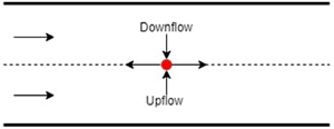
  $[H,1]$, respectively. The schematic of the flow geometry under consideration is shown in figure 1.

Figure 1. Schematic of a two-layer plane Poiseuille flow subjected to a wall-normal temperature gradient in scaled quantities. The velocity profile is shown for  $\mu _1 > \mu _2$. For $T_1 \neq T_2$, thermocapillary stresses develop along the interface due to the temperature dependence of the interface tension.
The velocity fields in the two fluids are  $\boldsymbol {v^{(i)}}=(v^{(i)}_x,v^{(i)}_y,v^{(i)}_z)$, where $i=1,2$ represent fluids $1$ and $2$, respectively. The dimensionless continuity equation is
 \begin{equation} \boldsymbol{\nabla} \boldsymbol{\cdot} \boldsymbol{v}^{(i)} =0, \end{equation}
where the gradient operator is  $\boldsymbol {\nabla }=\boldsymbol {e}_x \partial _ x+ \boldsymbol {e}_y \partial _y + \boldsymbol {e}_z \partial _z$, with $\boldsymbol {e}_j$ denoting the unit vector in the $j$ direction. The dimensionless Navier–Stokes equations for the fluids are
 \begin{equation} Re [\partial_t \boldsymbol{v^{(i)}}+(\boldsymbol{v^{(i)}} \boldsymbol{\cdot} \boldsymbol{\nabla}) \boldsymbol{v^{(i)}}]={-}\boldsymbol{\nabla} p^{(i)} + \mu^{(i)} {\nabla}^{2} \boldsymbol{v^{(i)}}, \end{equation}
in which  $Re\equiv \rho V_I R/\mu _1$ is the Reynolds number and ${\nabla }^2\equiv \partial _x^2+\partial _y^2+\partial _z^2$ is the Laplacian operator. The dimensionless viscosities are $\mu ^{(1)}=1$ for fluid $1$ and $\displaystyle \mu ^{(2)}=\mu _r \equiv \mu _2/\mu _1$ for fluid $2$. The dimensionless energy equations are
 \begin{equation} Re\,Pr [\partial_t T^{(i)}+(\boldsymbol{v^{(i)}} \boldsymbol{\cdot} \boldsymbol{\nabla}) T^{(i)}]= \kappa^{(i)} {\nabla}^{2} T^{(i)}, \end{equation}
where  $Pr=\mu _1 c_p/\kappa _1$ is the Prandtl number based on the properties of fluid 1. The dimensionless thermal conductivities are $\kappa ^{(1)}=1$ for fluid $1$ and $\kappa ^{(2)}=\kappa _r \equiv \kappa _2/\kappa _1$ for fluid $2$.
$2$.
The governing equations (2.2) are subjected to the following boundary conditions. Assuming no-slip, impermeable plates and fixed temperatures at the bounding plates yield
 $$\begin{gather} v^{(1)}_x=0; \quad v^{(1)}_y=0; \quad v^{(1)}_z=0; \quad T^{(1)}=T_1, \quad \text{at} \ y=0, \end{gather}$$
 $$\begin{gather}v^{(2)}_x=0; \quad v^{(2)}_y=0; \quad v^{(2)}_z=0; \quad T^{(2)}=T_2, \quad \text{at} \ y=1. \end{gather}$$
For the linear stability analysis, the assumption of two-dimensional disturbances is not applicable for the present system due to the thermocapillarity, which can excite spanwise unstable modes earlier than the streamwise modes implying inapplicability of the Squire's theorem (Pearson Reference Pearson1958). Thus, henceforth three-dimensional disturbances will be considered for the stability analysis. The fluid–fluid interface is located at  $y=H+\xi (x,t)$, where $\xi (x,t)$ is the infinitesimal displacement of the interface from its undisturbed position, $y=H$. The boundary conditions at the interface are the kinematic boundary condition, the balance of the tangential and normal components of the velocities and stresses, as well as the balance of the temperature and heat flux, as follows:
 $$\begin{gather} \partial_t \xi +v_x \partial_x \xi = v_y, \end{gather}$$
 $$\begin{gather}\boldsymbol{v}^{(1)} - \boldsymbol{v}^{(2)} =0, \end{gather}$$
 $$\begin{gather}\boldsymbol{t_1} \boldsymbol{\cdot} \boldsymbol{\tau}^{(1)} \boldsymbol{\cdot} \boldsymbol{n} - \boldsymbol{t_1} \boldsymbol{\cdot} \boldsymbol{\tau}^{(2)} \boldsymbol{\cdot} \boldsymbol{n}={-} Ma \boldsymbol{\nabla} T \boldsymbol{\cdot} \boldsymbol{t_1}, \end{gather}$$
 $$\begin{gather}\boldsymbol{t_2} \boldsymbol{\cdot} \boldsymbol{\tau}^{(1)} \boldsymbol{\cdot} \boldsymbol{n} - \boldsymbol{t_2} \boldsymbol{\cdot} \boldsymbol{\tau}^{(2)} \boldsymbol{\cdot} \boldsymbol{n}={-} Ma \boldsymbol{\nabla} T \boldsymbol{\cdot} \boldsymbol{t_2}, \end{gather}$$
 $$\begin{gather}-p^{(1)} \, + \boldsymbol{n} \boldsymbol{\cdot} \boldsymbol{\tau}^{(1)} \boldsymbol{\cdot} \boldsymbol{n} - ({-}p^{(2)} \, + \boldsymbol{n} \boldsymbol{\cdot} \boldsymbol{\tau}^{(2)} \boldsymbol{\cdot} \boldsymbol{n})={-}Ca^{{-}1} (\boldsymbol{\nabla} \boldsymbol{\cdot} \boldsymbol{n}), \end{gather}$$
 $$\begin{gather}T^{(1)} - T^{(2)} =0, \end{gather}$$
 $$\begin{gather}\boldsymbol{\nabla} T^{(1)} \boldsymbol{\cdot} \boldsymbol{n} - \kappa_r \boldsymbol{\nabla} T^{(2)} \boldsymbol{\cdot} \boldsymbol{n} = 0. \end{gather}$$
Here  $Ca={\mu _1 V_I}/{\sigma _0}$ is the capillary number and $Ma={\gamma \beta HR}/{\mu _1 V_I}$ is the Marangoni number. By definition, the sign of $Ma$ is the same as that of the base-state temperature gradient across fluid 1, i.e. $\beta$. The Marangoni number can be rearranged as
 \begin{equation} Ma=\frac{\gamma \beta}{\mu_1 V_I/(HR)}=\frac{\text{Thermocapillary stress at the interface due to fluid 1}}{\text{Viscous stress at the interface due to fluid 1}}. \end{equation}
Thus, the Marangoni number defined here gives relative importance of the thermocapillary and viscous stresses due to fluid 1 along the interface.
The vectors  $\boldsymbol {t_1}$, $\boldsymbol {t_2}$ and $\boldsymbol {n}$ represent the unit tangent and normal vectors to the free surface, respectively. The linearised expressions for the normal and tangential vectors at the free surface in the perturbed state are
 \begin{equation} \boldsymbol{n}={-}\partial_x \xi \boldsymbol{e_x} + \boldsymbol{e_y} - \partial_z \xi \boldsymbol{e_z}; \quad \boldsymbol{t_1}=\boldsymbol{e_x} + \partial_x \xi \boldsymbol{e_y}; \quad \boldsymbol{t_2}=\boldsymbol{e_z} + \partial_z \xi \boldsymbol{e_y}. \end{equation}
2.1. Base state
A steady-state, fully developed pressure-driven bilayer flow has base-state velocities
 $$\begin{gather} \bar{v}_x^{(1)}= \frac{y [y-1 - H (\mu_r-1) (H - y)]}{(H-1) H}, \end{gather}$$
 $$\begin{gather}\bar{v}_x^{(2)}= \frac{(y-1) [y-H (\mu_r-1) (H -1 - y)]}{(H-1) H\mu_r}. \end{gather}$$
Similarly, the base-state temperature gradients are
 $$\begin{gather} \frac{\partial \bar{T}^{(1)}}{\partial y}=1; \quad \frac{\partial \bar{T}^{(2)}}{\partial y} = \frac{1}{\kappa_r}, \end{gather}$$
 $$\begin{gather}\beta_1 = \frac{\kappa_2 (T^*_2 - T^*_1)}{[(1-H)\kappa_1+ H \kappa_2] R}. \end{gather}$$
The subsequent linear stability analysis is performed with respect to this base state.
2.2. Linearised perturbation equations
For the linear stability analysis, dynamical quantities such as velocities, temperatures and pressures are decomposed into the base-state and perturbed state, as  ${\mathcal {F}}(\boldsymbol {x},t)=\bar {\mathcal {F}}(y)+{\mathcal {F}}'(\boldsymbol {x},t)$. Here, ${\mathcal {F}}(\boldsymbol {x},t)$ is any dynamic quantity and a prime signifies the small perturbation quantity. In the linearised governing equations, the normal modes of the following form are then substituted:
 \begin{equation} {\mathcal{F}}'(\boldsymbol{x},t)=\tilde{\mathcal{F}}(y) \exp({{\rm i} (k x + m z - \omega t)}). \end{equation}
Here  $k$ and $m$ are the wavenumbers and $\tilde {\mathcal {F}}(y)$ is the eigenfunction of ${\mathcal {F}}'(\boldsymbol {x},t)$. The other parameter, $\omega =\omega _r+ {\rm i} \omega _i$, is the complex frequency, which characterises the temporal phase speed and growth of the disturbances. For the temporal stability analysis, the wavenumbers are treated as real numbers, while for the spatio-temporal analysis, the wavenumbers are complex numbers. The flow is considered temporally unstable if at least one eigenvalue satisfies the condition $\omega _i>0$. As described in § 6.2, the flow is absolutely unstable if the imaginary part of the complex frequency at the cusp point ( $\omega _{i0}$) satisfies the condition $\omega _{i0}>0$, otherwise, convectively unstable. After the substitution of the normal modes, the linearised governing equations become
 $$\begin{gather} {\rm i} k \tilde v^{(i)}_x + D \tilde v^{(i)}_y=0, \end{gather}$$
 $$\begin{gather}Re [ -{\rm i} \omega \tilde v^{(i)}_x + {\rm i} k \bar v^{(i)}_x \tilde v^{(i)}_x + \tilde v^{(i)}_y D \bar v^{(i)}_x] ={-}{\rm i} k \tilde p^{(i)} + \mu^{(i)} (D^{2}-k^{2}-m^2) \tilde v^{(i)}_x, \end{gather}$$
 $$\begin{gather}Re [ -{\rm i} \omega \tilde v^{(i)}_y + {\rm i} k \bar v^{(i)}_x \tilde v^{(i)}_y ] ={-}D \tilde p^{(i)} + \mu^{(i)} (D^{2}-k^{2}-m^2) \tilde v^{(i)}_y, \end{gather}$$
 $$\begin{gather}Re [ -{\rm i} \omega \tilde v^{(i)}_z + {\rm i} k \bar v^{(i)}_x \tilde v^{(i)}_z ] ={-}{\rm i}m \tilde p^{(i)} + \mu^{(i)} (D^{2}-k^{2}-m^2) \tilde v^{(i)}_z, \end{gather}$$
 $$\begin{gather}Re\, Pr [ -{\rm i} \omega \tilde T^{(i)} + {\rm i} k \bar v^{(i)}_x \tilde T^{(i)} + D \bar T^{(i)} \tilde v^{(i)}_y] = \kappa^{(i)} (D^{2}-k^{2}-m^2) \tilde T^{(i)}, \end{gather}$$
where  $D={\rm d}/{{\rm d} y}$.
The above equations are to be solved using the following boundary conditions. At  $y=0$ and $y=1$, the assumption of no-slip, impermeability and imposed temperature gradient along the plates gives
 $$\begin{gather} \tilde v^{(1)}_x =0; \quad \tilde v^{(1)}_y =0; \quad \tilde v^{(1)}_z =0; \quad \tilde T^{(1)} =0, \quad \text{at} \ y=0, \end{gather}$$
 $$\begin{gather}\tilde v^{(2)}_x =0; \quad \tilde v^{(2)}_y =0; \quad \tilde v^{(2)}_z =0; \quad \tilde T^{(2)} =0, \quad \text{at} \ y=1. \end{gather}$$
 At  $y=H$, oscillations of the fluid–fluid interface will be induced due to the perturbations. Thus, the infinitesimal displacement of the interface will play a role. These boundary conditions, after substitution of the normal modes, become
 \begin{gather} {\rm i} (k\bar v^{(1)}_x -\omega) \tilde \xi = \tilde v^{(1)}_y , \end{gather}
 \begin{gather} \tilde v^{(1)}_x + D \bar v^{(1)}_x \tilde \xi = \tilde v^{(2)}_x + D \bar v^{(2)}_x \tilde \xi, \end{gather}
 \begin{gather} \tilde v^{(1)}_y = \tilde v^{(2)}_y, \end{gather}
 \begin{gather} \tilde v^{(1)}_z = \tilde v^{(2)}_z, \end{gather}
 $$\begin{gather} D \tilde v^{(1)}_x + {\rm i}k \tilde v^{(1)}_y + [ D^2 \bar v^{(1)}_x - \mu_r D^2 \bar v^{(2)}_x ] \tilde \xi \nonumber\\ =\mu_r ( D \tilde v^{(2)}_x + {\rm i}k \tilde v^{(2)}_y) - {\rm i} k Ma (\tilde T^{(1)} + D \bar T^{(1)} \tilde\xi), \end{gather}$$
 \begin{gather} D \tilde v^{(1)}_z + {\rm i}m \tilde v^{(1)}_y = \mu_r (D \tilde v^{(2)}_z + {\rm i}m \tilde v^{(2)}_y) - {\rm i} m Ma (\tilde T^{(1)} + D \bar T^{(1)} \tilde \xi), \end{gather}
 \begin{gather} -\tilde p^{(1)} + 2 D v^{(1)}_y ={-}\tilde p^{(2)} + 2 \mu_r D v^{(2)}_y - Ca^{{-}1} (k^2+m^2) \tilde \xi, \end{gather}
 \begin{gather} \tilde T^{(1)} + D \bar T^{(1)} \tilde \xi = \tilde T^{(2)} + D \bar T^{(2)} \tilde \xi, \end{gather}
 \begin{gather} D\tilde T^{(1)} = \kappa_r D \tilde T^{(2)}, \end{gather}
where all quantities are evaluated at  $y=H$.
3. Numerical approach
To carry out the GLSA of the problem at hand, the pseudo-spectral method is employed in which the eigenfunctions corresponding to each dynamic field are expanded into a series of Chebyshev polynomials as
 \begin{equation} \tilde{f}(y)=\sum_{m=0}^{m=N} a_m {\mathcal{T}}_m (y), \end{equation}
where  ${\mathcal {T}}_m(y)$ are Chebyshev polynomials of degree $m$ and $N$ is the highest degree of the polynomial in the series expansion or, equivalently, the number of collocation points. The series coefficients $a_m$ are the unknowns to be solved for. The generalized eigenvalue problem is constructed in the form
 \begin{equation} \boldsymbol{A}\boldsymbol{e} + \omega \boldsymbol{B}\boldsymbol{e}=0, \end{equation}
where  $\boldsymbol {A}$ and $\boldsymbol {B}$ are matrices obtained from the discretisation procedure and $\boldsymbol {e}$ is the vector containing the coefficients of all series expansions.
The details of the discretisation of the governing equations and boundary conditions, and construction of  $\boldsymbol {A}$ and $\boldsymbol {B}$ can be found in the standard procedure described by Trefethen (Reference Trefethen2000) and Schmid & Henningson (Reference Schmid and Henningson2001). Application of the pseudo-spectral method for similar problems can be found in the study of Boomkamp et al. (Reference Boomkamp, Boersma, Miesen and Beijnon1997), Barmak et al. (Reference Barmak, Gelfgat, Vitoshkin, Ullmann and Brauner1994), Patne, Agnon & Oron (Reference Patne, Agnon and Oron2020, Reference Patne, Agnon and Oron2021); Patne et al. (Reference Patne, Agnon, Oron and Ramon2022). The MATLAB routine eig is used to solve the constructed generalized eigenvalue problem equation (3.2).
To identify genuine modes in the numerically computed spectrum, the eigenspectrum is obtained for  $N$ and $N+2$ collocation points, which are then compared with a specified tolerance, e.g. $10^{-4}$. The genuine eigenvalues are further verified by increasing the number of collocation points by $25$ and monitoring the variation of the obtained eigenvalues. If the eigenvalue does not change up to a prescribed precision, e.g. to the sixth significant digit, the same number of collocation points are used to determine the critical parameters of the system. In the present work, $N=50$ is found to be sufficient to achieve convergence and determine the leading, most unstable eigenvalue within the investigated parameter range.
It must be noted that the numerical and analytical approaches employed here are similar to the one used for studying the stability of a non-isothermal two-layer plane Couette flow by Patne et al. (Reference Patne, Agnon, Oron and Ramon2022). Additionally, for an isothermal two-layer Poiseuille flow, we have validated the asymptotic approach against the standard procedure developed by Yih (Reference Yih1967) and Yiantsios & Higgins (Reference Yiantsios and Higgins1988) as follows.
To standardise and compare with their predictions, the layers are assumed to be of equal thickness, the relation  $\omega = k c$ is used, and the coordinate system origin is shifted to the fluid–fluid interface so that the interface lies at $y=0$ and fluids 1 and 2 will be present in the intervals $[0,1]$ and $[0,-1]$, respectively. This adjustment then modifies the base state (2.6) and boundary conditions (2.3) location to mimic Yih (Reference Yih1967) and Yiantsios & Higgins (Reference Yiantsios and Higgins1988). Now following the procedure for the long-wave asymptotic analysis outlined in § 4, we obtain
 \begin{equation} c_0 = 1 + \frac{2(\mu_r -1)^2}{\mu_r^2 + 14\mu_r + 1} \end{equation}
in exact agreement with equation (46) of Yih (Reference Yih1967) and equation (9) of Yiantsios & Higgins (Reference Yiantsios and Higgins1988) for  $n=1$. Please note that they use $m$ to denote the viscosity ratio $\mu _r$ and $n$ to denote the thickness ratio $H$. Next, we proceed with the $O(k)$ eigenvalue correction for which term-by-term comparison is difficult, thus, the unstable eigenvalue for a particular value of $\mu _r$ is compared. For $n=1$ and $m = 10$, the continuous curve in figure 2(a) of Yiantsios & Higgins (Reference Yiantsios and Higgins1988) gives $c_1/(k Re) \sim 0.0128$ while our procedure followed here predicts $c_1//(k Re)= 0.0127$, which is in excellent agreement thereby validating the long-wave asymptotic analysis. The results obtained by the numerical calculations are then verified against the predictions of the standardised long-wave asymptotic analysis, as shown in figure 4, thus validating the former.
4. General linear stability analysis
Before proceeding with the results, an estimation of the practical range of the dimensionless parameters is presented here. In this case, the typical ranges for the physical properties are (Ezersky et al. Reference Ezersky, Garcimartin, Mancini and Perez-Garcia1993; De Saedeleer et al. Reference De Saedeleer, Garcimartin, Chavepeyer, Platten and Lebon1996; Li, Xu & Kumacheva Reference Li, Xu and Kumacheva2000; Schatz & Neitzel Reference Schatz and Neitzel2001; Ospennikov & Schwabe Reference Ospennikov and Schwabe2004; Mizev & Schwabe Reference Mizev and Schwabe2009)  $R \sim 10^{-6}-10^{-2}$ m, $\rho \sim 10^{3}$ kg m $^{-3}$, $\sigma _0 \sim 10^{-3}-10^{-1}$ N m $^{-1}$, $\gamma \sim 10^{-5}-10^{-3}$ N (m K) $^{-1}$, $\kappa \sim 10^{-2}-10^{2}$ J (m s K) $^{-1}$, $\mu \sim 10^{-5}-10^{2}$ Pa s and $V_I \sim 10^{-3}-10^{-1}$ m s $^{-1}$. Thus, the typical dimensionless numbers are $Re \sim O(10^{-5}-10^{3}), Ca \sim O(10^{-4}-10^{-1})$ and $Pr \sim O(10^{-3}-10^{3})$. This parametric range will be used here to study the predicted instabilities.
As explained in § 1, the thermocapillary stresses exerted by the fluid layers exhibit strong competition and may influence the stability of the flow. Figure 2 shows the strong destabilising effect of the thermocapillary stresses, which results in instability. The role of the thermocapillary stresses along the interface becomes clear from figure 3. Additionally, figure 3(b) shows that as  $k\ll 1$, the growth rate $\omega _i \neq 0$, thereby illustrating the long-wave nature of the instability. Figures 2 and 3 show the streamwise mode ( $m=0$). A similar spanwise unstable mode ( $k=0$) also exists with $\omega _r=0$, thus, a stationary mode. The long-wave streamwise and spanwise modes are amenable to the asymptotic approach with asymptotic expansion around the limit $k=m=0$. For the convenience of the mathematical analysis and presentation of the results, the discussion will be divided into two sections dealing with the streamwise and spanwise modes.

Figure 2. The effect of the variation in  $Ma$ on the streamwise mode in the $\omega _r - \omega _i$ plane at $Re=10, H=0.4, \mu _r=0.5, \kappa _r=1, k=0.1, Ca=0.001,m=0,$ and $Pr=7$. The eigenvalues in the figure correspond to a decreasing $Ma$ in steps of unity such that the blue circle with $\omega _i<0$ is for $Ma=0$ and the star with $\omega _i>0$ is for $Ma=-5$. The figure demonstrates the strong destabilising effect of the thermocapillary stresses on the growth rate of the unstable mode.

Figure 3. The variation of  $\omega _i$ with $k$ for the streamwise mode at $Re=10, H=0.4, \mu _r=0.5, $ $\kappa _r=1, Ca=0.001,m=0$ and $Pr=7$. Panel (a) shows the destabilising effect of decreasing $Ma$ on the streamwise mode. Panel (b) provides the magnified view of the streamwise mode at low $k$ to show that $\omega _i \neq 0$ for $k\ll 1$, thereby illustrating the long-wave nature of the streamwise mode.
4.1. Streamwise mode ( $m=0$)

For  $m=0$ and $\tilde v_z =0$, the momentum perturbation equations in (2.8) can be reduced to two-dimensional Orr–Sommerfeld equations
 \begin{equation} {\rm i} Re (k \bar
v_x^{(i)} - \omega ) ( D^2 - k^2 ) \tilde
v_y^{(i)} = \mu^{(i)} ( D^2 - k^2 )^2 \tilde
v_y^{(i)} - {\rm i}k Re D^2 \bar v_x^{(i)}\tilde v_y^{(i)},
\end{equation}
\begin{equation} {\rm i} Re (k \bar
v_x^{(i)} - \omega ) ( D^2 - k^2 ) \tilde
v_y^{(i)} = \mu^{(i)} ( D^2 - k^2 )^2 \tilde
v_y^{(i)} - {\rm i}k Re D^2 \bar v_x^{(i)}\tilde v_y^{(i)},
\end{equation}
whereas the energy equation in (2.8) is modified by substituting  $m=0$. Next, the velocity and temperature fields and the complex frequency $\omega$ are expanded as the series in terms of a small wavenumber $k$, as
 $$\begin{gather} \tilde v_y^{(i)}= v_{y0}^{(i)} + k v_{y1}^{(i)} + k^2 v_{y2}^{(i)} +\cdots, \end{gather}$$
 $$\begin{gather}\omega=k c_0 + k^2 c_1 + k^3 c_2 +\cdots, \end{gather}$$
 $$\begin{gather}\tilde T^{(i)}= \frac{1}{k} T_{0}^{(i)} + T_{1}^{(i)} + k T_{2}^{(i)} +\cdots. \end{gather}$$
The above expansions are then substituted into the Orr–Sommerfeld equation (4.1), the energy equation (2.8e) and the boundary conditions (2.9). Similar expansion in powers of  $k$ for $\tilde v_x^{(i)}$ can be obtained from the continuity equations and, for $\tilde p^{(i)}$, can be obtained from the $x$-momentum equation.
At  $O(1)$, the governing equations read
 \begin{equation} D^4 v_{y0}^{(i)} = 0; \quad D^2 T_{0}^{(i)} = 0. \end{equation}
Using the expansions (4.2), the  $O(1)$ eigenvalue is
 \begin{equation} c_0 ={-}\frac{[(H^2-2H) (\mu_r-1)-1] [1 + H^2 (\mu_r-1)]}{1 + H (\mu_r -1) [4 - 6 H + 4 H^2 - H^3 + H^3 \mu_r] }. \end{equation}
The  $O(1)$ eigenvalue, $c_0$, is a real quantity, thus, these are purely travelling disturbances. For $H=0.5$, the above expression reduces to equation (46) of Yih (Reference Yih1967), thereby validating the procedure. The above expression is independent of the capillary number $Ca$ in agreement with Yih (Reference Yih1967). Furthermore, $c_0$ for both the flows is independent of $\kappa _r$, representing the thermal conductivity stratification, and $Ma$, reflecting the thermal stresses. This implies that the thermocapillarity and thermal properties do not affect the phase speed of the disturbances, while they might affect at $O(k)$ or higher. Thus, we proceed with higher-order correction, i.e. $O(k)$.
At  $O(k)$, the governing equations are
 $$\begin{gather} \mu^{(i)} D^4 v_{y1}^{(i)} + {\rm i} Re (c_0 - \bar v_{x}^{(i)}) D^2 v_{y0}^{(i)} - Re D^2 \bar v_{x}^{(i)} v_{y0}^{(i)}= 0, \end{gather}$$
 $$\begin{gather}\kappa^{(i)} D^2 T_{1}^{(i)} + {\rm i} Re\,Pr ( c_0 - \bar v_{x}^{(i)}) T_{0}^{(i)} - Re\,Pr D \bar T^{(i)} v_{y0}^{(i)} = 0. \end{gather}$$
Solving (4.5) in the same way as for  $O(1)$ above, yields
 \begin{equation} c_1={\rm i} \, [ f_1 (H,\mu_r, \kappa_r) \, Ma + f_2 (H,\mu_r) \, Re], \end{equation}
where
 $$\begin{gather} f_1=\frac{g_1}{g_2}; \quad f_2 = \frac{g_3}{g_4}, \end{gather}$$
 $$\begin{gather}g_1 = (H-1)^2 H^2 (2 H - H^2 + \mu_r H^2 - 1), \end{gather}$$
 $$\begin{gather}g_2 = [1 + (\kappa_r-1)
H] \, [2 + 2 H (\mu_r-1) (4 - 6 H + 4 H^2 - H^3 + \mu_r
H^3)],\\ g_3 ={-}(2 H \,{-}\, H^2 + \mu_r
H^2-1) \{1 \,{-}\, \mu_r + 5 H^{14} (\mu_r\,{-}\,1)^7 (1 + \mu_r) + 2 H
({-}4 + 3 \mu_r + \mu_r^2)\nonumber\\ -2 H^{13} (\mu_r-1)^6
({-}32 + 19 \mu_r + 3 \mu_r^2) + H^{12} (\mu_r-1)^5 (377 -
694 \mu_r + 177 \mu_r^2) \nonumber\\ +H^2 (13 + 4 \mu_r +
15 \mu_r^2 - 32 \mu_r^3) + 8 H^3 (13 - 34 \mu_r + 16
\mu_r^2 + 5 \mu_r^3) \nonumber\\ -8 H^{11} (\mu_r-1)^4
({-}169 + 472 \mu_r - 258 \mu_r^2 + 29 \mu_r^3) \nonumber\\
-2 H^5 (\mu_r-1)^2 ({-}1144 + 1441 \mu_r - 1107 \mu_r^2 +
112 \mu_r^3) \nonumber\\ +2 H^9 (\mu_r-1)^3 ({-}2860 + 8635
\mu_r - 4718 \mu_r^2 + 223 \mu_r^3) \nonumber\\ +H^8
(\mu_r-1)^3 (7293 - 17490 \mu_r + 5341 \mu_r^2 + 472
\mu_r^3) \nonumber\\ +H^6 (\mu_r-1)^2 ({-}4719 + 9240 \mu_r
- 6473 \mu_r^2 + 776 \mu_r^3)\nonumber\\ +H^4 ({-}715 +
1925 \mu_r - 2061 \mu_r^2 + 1259 \mu_r^3 - 408 \mu_r^4)
\nonumber\\ -16 H^7 (\mu_r-1)^2 ({-}429 + 1155 \mu_r - 873
\mu_r^2 + 112 \mu_r^3 + 14 \mu_r^4) \nonumber\\ +H^{10}
(\mu_r-1)^3 (3289 - 11517 \mu_r + 9743 \mu_r^2 - 2115
\mu_r^3 + 88 \mu_r^4)\},
\end{gather}$$
$$\begin{gather}g_2 = [1 + (\kappa_r-1)
H] \, [2 + 2 H (\mu_r-1) (4 - 6 H + 4 H^2 - H^3 + \mu_r
H^3)],\\ g_3 ={-}(2 H \,{-}\, H^2 + \mu_r
H^2-1) \{1 \,{-}\, \mu_r + 5 H^{14} (\mu_r\,{-}\,1)^7 (1 + \mu_r) + 2 H
({-}4 + 3 \mu_r + \mu_r^2)\nonumber\\ -2 H^{13} (\mu_r-1)^6
({-}32 + 19 \mu_r + 3 \mu_r^2) + H^{12} (\mu_r-1)^5 (377 -
694 \mu_r + 177 \mu_r^2) \nonumber\\ +H^2 (13 + 4 \mu_r +
15 \mu_r^2 - 32 \mu_r^3) + 8 H^3 (13 - 34 \mu_r + 16
\mu_r^2 + 5 \mu_r^3) \nonumber\\ -8 H^{11} (\mu_r-1)^4
({-}169 + 472 \mu_r - 258 \mu_r^2 + 29 \mu_r^3) \nonumber\\
-2 H^5 (\mu_r-1)^2 ({-}1144 + 1441 \mu_r - 1107 \mu_r^2 +
112 \mu_r^3) \nonumber\\ +2 H^9 (\mu_r-1)^3 ({-}2860 + 8635
\mu_r - 4718 \mu_r^2 + 223 \mu_r^3) \nonumber\\ +H^8
(\mu_r-1)^3 (7293 - 17490 \mu_r + 5341 \mu_r^2 + 472
\mu_r^3) \nonumber\\ +H^6 (\mu_r-1)^2 ({-}4719 + 9240 \mu_r
- 6473 \mu_r^2 + 776 \mu_r^3)\nonumber\\ +H^4 ({-}715 +
1925 \mu_r - 2061 \mu_r^2 + 1259 \mu_r^3 - 408 \mu_r^4)
\nonumber\\ -16 H^7 (\mu_r-1)^2 ({-}429 + 1155 \mu_r - 873
\mu_r^2 + 112 \mu_r^3 + 14 \mu_r^4) \nonumber\\ +H^{10}
(\mu_r-1)^3 (3289 - 11517 \mu_r + 9743 \mu_r^2 - 2115
\mu_r^3 + 88 \mu_r^4)\},
\end{gather}$$
 $$\begin{gather}g_4 = 420 (1 + H (4 - 6
H + 4 H^2 - H^3 + \mu_r H^4) (\mu_r-1))^3 \mu_r^2.
\end{gather}$$
$$\begin{gather}g_4 = 420 (1 + H (4 - 6
H + 4 H^2 - H^3 + \mu_r H^4) (\mu_r-1))^3 \mu_r^2.
\end{gather}$$
Using (4.4) and (4.6), the eigenvalue  $\omega$ up to $O(k)$ correction is
 \begin{equation} \omega=k c_0(H,\mu_r)+{\rm i} \, k^2 \, [ f_1 (H,\mu_r, \kappa_r) \, Ma + f_2 (H,\mu_r) \, Re ]. \end{equation}
The function  $f_1 (H,\mu _r, \kappa _r)$ represents the combined effect of the thermocapillarity and viscosity stratification along the interface while the function $f_2 (H,\mu _r)$ represents the inertial stresses alone. The function $f_2 (H,\mu _r)$ is similar to the coefficient of $Re$ in the analysis of Yih (Reference Yih1967), thus representing the shear-flow instability due to the viscosity stratification in the absence of an imposed temperature gradient. The first function $f_1 (H,\mu _r, \kappa _r)$ is dependent on both the viscosity and thermal conductivity stratification and represents an additional term due to the imposed temperature gradient. Clearly, the mechanism responsible for the instability stems from shearing action ( $Re$ term) along the interface, which results in the ‘shear-flow mode’ and thermocapillary stresses ( $Ma$ term) along the interface, which leads to the ‘thermocapillary mode’. Additionally, from (4.8), the long-wave instability is independent of $Pr$, which is present only in the energy equation as a coefficient of the convection term. Thus, although the momentum convection terms affect the long-wave instability (through the $Re$ term), the energy convection does not affect the long-wave instability. The effect of the energy appears only through the Marangoni terms implying the vital role played by the thermocapillary stresses (through the $Ma$ term) in determining the stability of the flow.
From (4.8), the instability can exist ( $\omega _i >0$) for an arbitrary $Re$ and $Ma>0$ if $f_1 >0$ and $f_2 >0$. When $f_1>0$ and $f_2<0$, then a minimum value of $Ma>0$ will be necessary to set in the instability. If $f_1<0$ and $f_2>0$ then the flow is unconditionally unstable for $Ma<0$, implying the necessity of a negative temperature gradient across fluid 1. For $f_1<0$ and $f_2<0$, a minimum value of $Ma<0$ is necessary to make flow unstable. Thus, the rest of the analysis aims to evaluate the required critical value and sign of the critical Marangoni number $Ma_c$ to stabilise/destabilise the flow. Equating the imaginary part of (4.8) to zero, we obtain the expression for the critical Marangoni number
 \begin{equation} Ma_c ={-}\frac{f_2 (H,\mu_r)}{f_1 (H,\mu_r, \kappa_r)} Re, \end{equation}
implying  $Re$ merely enters as a multiplier; thus, in the present study we have presented and discussed the results for the temporal instability for a fixed $Re=0.1$.
The comparison of the growth rate ( $\omega _i$) of the unstable streamwise mode predicted by the numerical approach and the asymptotic approach (4.6) is presented in figure 4. On expected lines, the asymptotic and numerical approaches are in excellent agreement for $k<0.5$. From the $O(k)$ expression for the eigenvalue, the shear-flow instability is independent of $Ca$. To accommodate this in the numerical approach, $Ca=\infty$ has been used.

Figure 4. Comparison between the asymptotic and numerical approaches in the prediction of the growth rate  $\omega _i$ with wavenumber $k$ at $Re=0.1, H=0.3, \mu _r=0.3, \kappa _r=3, Ca=\infty$ and $Pr=7$ for the return flow. The excellent agreement between the asymptotic and numerical approaches for $k<0.5$ validates the numerical methodology utilised here. For $\omega _i >0$, the flow is unstable.
The orthonormalised velocity and temperature perturbations for the streamwise mode are shown in figure 5. The eigenfunctions vanish at the boundaries of the channel, i.e.  $y=0$ and $y=1$ due to the impermeability condition and the absence of the temperature perturbations at the wall given by boundary conditions (2.9a) and (2.9b). Also, both the eigenfunctions achieve maximum at the interface, implying that the instability is driven by the shear and thermocapillary stresses at the interface.

Figure 5. The variation of the orthonormalised velocity and temperature eigenfunctions (for fluid 1) in the  $x$–
$x$– $y$ plane at $Re=10, Pr=7, \mu _r=0.5, H=0.4, \kappa _r=1, Ma=-10, Ca=0.001$ and $k=0.1$ for the streamwise mode $\omega = 0.111936 + 0.000924 \, {\rm i}$. The eigenfunctions exhibit maximum variation near $y=0.4$, i.e. the interface, indicating the destabilisation introduced by the shearing and thermocapillary stresses along the interface. The plotted eigenfunctions are the modulus or absolute value of the respective eigenfunctions.
The critical parameter curves (corresponding to  $\omega _i=0$) in $Ma_c - H$ parametric space as a function of $\mu _r$ and $\kappa _r$ are shown in figure 6. From (4.7a), (4.7b) and (4.7d), the factor $(2 H - H^2 + \mu _r H^2 - 1)$ is common in the numerator for both $f_1 (H,\mu _r, \kappa _r)$ and $f_2 (H,\mu _r)$ with $g_3$ having a negative sign preceding the factor, thus, both functions have a common root $H=({\sqrt {\mu _r}-1})/({\mu _r-1})$. The remaining factors of $g_1$, namely, $(H-1)^2$, $H^2$ and $g_2$ do not affect the sign of $f_1$ for $\mu _r <1$. Similarly, the remaining factors of $g_3$ and $g_4$ do not affect the sign of $f_2$. Thus, for a given value of $H$ and $\mu _r$, both functions will possess an opposite sign and their signs will switch at the root $H=({\sqrt {\mu _r}-1})/({\mu _r-1})$. This is precisely the case depicted in figure 6 with the location of the vertical line parallel to the $Ma_c$ axis indicating the root. For example, for $\mu _r =0.1$, the root is $H=0.76$ with $f_1>0$ and $f_2<0$ for $H<0.76$ and $f_1<0$ and $f_2>0$ for $H>0.76$ separated by a vertical line at $H=0.76$ in figure 6(a). Thus, for $Ma>0$, for $H<0.76$, the thermocapillarity stabilises while the shear force has a destabilising influence. The opposite is the case for $f_1<0$ and $f_2>0$ for $H>0.76$. Also, the root $H=({\sqrt {\mu _r}-1})/({\mu _r-1})$ is independent of $\kappa _r$, thus, variation in $\kappa _r$ does not affect the location of the vertical line shown in figure 6.

Figure 6. Variation in the critical Marangoni number  $Ma_c$ with the relative position of the interface $H$ at ${Re=0.1}$. The capillary number $Ca$ and Prandtl number $Pr$ do not affect the critical parameters for the long-wave instability, as seen in (4.8). (a) For $H<0.76$, $f_1<0$ and $f_2>0$; thus, the thermocapillarity has a stabilising effect (if $\beta _1>0$) while the shearing force has a destabilising effect. As a result, the flow is unstable for $Ma< Ma_c$. However, for $H>0.76$, $f_1>0$ and $f_2<0$, which leads to the swapping of the stable and unstable regimes. (b) For $H<0.24$, $f_1<0$ and $f_2<0$; thus, both thermocapillarity and the shearing force have a stabilising effect (if $\beta _1>0$). However, if $\beta _1 <0$ then the flow becomes unstable for $Ma<0$. For $H>0.24$, the shearing force has a destabilising effect, while thermocapillarity with $\beta _1$ has a stabilising effect. (c) A decreasing $\kappa _2$ or an increasing $\kappa _1$ shifts the neutral stability boundary to a lower $Ma$. (d) Illustrates the opposite scenario of panel (c). Results are shown for (a) $\kappa _r=1$ and $\mu _r=0.1$, (b) $\kappa _r=1$ and $\mu _r=10$, (c) $\kappa _r=0.1$ and $\mu _r=0.1$, (d) $\kappa _r=10$ and $\mu _r=0.1$.
For  $\mu _r>1$, as shown in figure 6(b), a negative temperature gradient is necessary to stabilise or destabilise the flow. In this case, functions $f_1$ and $f_2$ have $H=0.24$ as the common root. For $H<0.24$, both $f_1$ and $f_2$ are negative, thus, both the thermocapillary and inertial terms have a stabilising influence due to which a negative temperature gradient is necessary to set in the instability. While for $H>0.24$, both $f_1$ and $f_2$ are positive, thus, both the thermocapillary and inertial terms have a destabilising influence. A negative temperature gradient then becomes necessary to stabilise the flow. The physical mechanism of the stabilisation or destabilisation due to the viscosity stratification, i.e. impact of variation in the parameter $\mu _r$ is explained in § 5.
The effect of the thermal conductivity stratification on the stable and unstable zones in  $Ma_c-H$ parametric space is shown in figure 6(c,d). Figure 6(c) shows that if fluid 2 has a lower thermal conductivity than fluid 1, i.e. $\kappa _r<1$, then compared with the only viscosity stratification shown in figure 6(a), the critical parameter curves shift to a lower $Ma_c$ while the opposite occurs for $\kappa _r>1$. The physical picture of the impact of variation in the parameter $\kappa _r$ on the thermocapillary mode is discussed in § 5.
The analysis of Wei (Reference Wei2006), which considered a two-layer plane Couette flow subjected to a temperature gradient, assumed one of the fluid layers in the thin-film limit implied  $H \to 0$ or $H\to 1$. He concluded that the shear-flow mode could be stabilised for an arbitrary $H$ by the thermocapillary mode. However, from figure 6, for $\mu _r<1$, the thermocapillarity is unable to stabilise the flow as $H\to 0$ while, for $\mu _r>1$, again thermocapillarity is incapable of stabilising the flow as $H\to 1$. This implies that the analysis of Wei (Reference Wei2006) has limited applicability to a two-layer pressure-driven flow subjected to a temperature gradient. Furthermore, Wei (Reference Wei2006) predicted two neutral states when the interface tension is weak, but there is no such region found in the present analysis highlighting the difference between the two-layer planar Couette and pressure-driven flows or a possible failure of the thin-film assumption of Wei (Reference Wei2006).
4.2. Spanwise mode ($k=0$)

For  $k=0$ and $\tilde v_x = 0$, the momentum perturbation equations in (2.8) reduce to
 \begin{equation} -{\rm i} \omega \, Re
( D^2 - m^2) \tilde v_y^{(i)} = \mu^{(i)}
( D^2 - m^2)^2 \tilde v_y^{(i)},
\end{equation}
\begin{equation} -{\rm i} \omega \, Re
( D^2 - m^2) \tilde v_y^{(i)} = \mu^{(i)}
( D^2 - m^2)^2 \tilde v_y^{(i)},
\end{equation}
and the energy equations in (2.8) are modified by substituting  $k=0$ and $\tilde v_x = 0$. Similar to the case of the streamwise perturbations, the velocity and temperature fields and the complex frequency $\omega$ are expanded as the series in terms of spanwise wavenumber $m$,
$m$,
 $$\begin{gather} \tilde v_y^{(i)}= v_{y0}^{(i)} + m v_{y1}^{(i)} + m^2 v_{y2}^{(i)} +\cdots, \end{gather}$$
 $$\begin{gather}\omega=m c_0 + m^2 c_1 + m^3 c_2 +\cdots, \end{gather}$$
 $$\begin{gather}\tilde T^{(i)}= \frac{1}{m} T_{0}^{(i)} + T_{1}^{(i)} + m T_{2}^{(i)} +\cdots. \end{gather}$$
The above expansions are then substituted in (4.10), the energy equation (2.8e) for  $k=0$ and the boundary conditions (2.9). The expansions in powers of $m$ for $\tilde v_x^{(i)}$ and $\tilde p^{(i)}$ are obtained from the continuity equations and the $z$-momentum equations, respectively.
At  $O(1)$, the governing equations read
 \begin{equation} D^4 v_{y0}^{(i)} = 0; \quad D^2 T_{0}^{(i)} = 0. \end{equation}
At  $O(1)$, the eigenvalue is
 \begin{equation} c_0 = 0. \end{equation}
This shows that the spanwise mode is stationary. At  $O(m)$, the governing equations are
 $$\begin{gather} \mu^{(i)} D^4 v_{y1}^{(i)} + {\rm i} Re c_0 D^2 v_{y0}^{(i)} = 0, \end{gather}$$
 $$\begin{gather}D^2 T_{1}^{(i)} + {\rm i} Re\,Pr c_0 T_{0}^{(i)} - Re\,Pr \frac{\partial \bar T^{(i)}}{ \partial y} v_{y0}^{(i)} = 0. \end{gather}$$
Solving (4.16) in the same way as for  $O(1)$ above, yields
 \begin{equation} c_1={\rm i} \, f_1(H,\mu_r, \kappa_r) \, Ma, \end{equation}
where  $f_1$ is a function defined in (4.7a). Using (4.15) and (4.17), the eigenvalue $\omega$ up to $O(m)$ correction is
 \begin{equation} \omega={\rm i} \, m^2 \, f_1(H,\mu_r, \kappa_r) \, Ma. \end{equation}
A comparison of the above expression for  $\omega$ with the expression for the complex frequency for the streamwise mode (4.8) shows the absence of the shear-flow term (i.e. $Re$ term) for the spanwise mode. The shear-flow term is absent since the base-state flow is only in the streamwise direction, while there is no base-state velocity present in the spanwise direction. This is also the reason that the $O(1)$ eigenvalue vanishes, thereby implying a stationary mode.
From (4.18), the spanwise mode is unstable if the product  $f_1 Ma > 0$. From figure 7(a), for a given $\mu _r$, there exists a range of $H$ for which $f_1>0$. For such a range, the spanwise perturbations become unstable for a positive temperature gradient, i.e. $Ma>0$. While for $f_1<0$, a negative temperature gradient, i.e. $Ma<0$, is essential for destabilising the spanwise mode. For example, from the curve for $\mu _r=0.1$, $f_1<0$ for $H<0.76$ and $f_1>0$ for $H>0.76$; thus, to destabilise the spanwise perturbations, $Ma<0$ for $H<0.76$ and $Ma>0$ for $H>0.76$ will be necessary.

Figure 7. Variation of the function  $f_1$ with the relative position of the liquid–liquid interface $H$. (a) An increasing $\mu _r$ increases the range of $H$ for which $f_1>0$. (b) A decreasing $\kappa _r$ increases maximum $|f_1|$ values. The spanwise mode is unstable for the $H$ range that satisfies the condition $f_1 > 0$. Results are shown for (a) $\kappa _r=1$, (b) $\mu _r=0.1$.
The dominant mode of instability, i.e. the mode with the higher growth rate between the streamwise and spanwise modes, and its range can be decided as follows. When  $f_2<0$, then from (4.8), the streamwise mode will have to overcome the stabilising effect of the inertial term to destabilise the flow, which is not the case with the spanwise mode since the inertial term is absent (see (4.18)). Thus, the spanwise mode will dominate the stability of the flow in the parametric regime for which $f_2<0$. The opposite is true when the inertial term has a destabilising effect, i.e. $f_2>0$. In this case, the streamwise mode will have a higher growth rate than the spanwise mode, thereby becoming the dominant mode.
4.3. Oblique modes
The above discussion was limited to only the extremes, i.e. streamwise and spanwise instability modes. However, the streamwise and spanwise instability modes turn out to be the dominant modes of instability as follows. A comparison of (4.8) and (4.18) shows that the difference between the two modes is due to the term  $f_2(H,\mu _r) Re$. Thus, if $f_2<0$ then the spanwise mode will possess a higher growth rate than the streamwise mode, and the opposite will be true for $f_2>0$. Any oblique mode with $k \neq 0$ and $m\neq 0$ will have both $Ma$ and $Re$ terms. The function $f_1$ will remain the same for all oblique modes since it remains the same for the extremes, i.e. streamwise and spanwise modes. However, the $Re$ term will diminish as one goes from a streamwise to spanwise mode. Thus, if $f_2<0$, all oblique and streamwise modes will have a growth rate lower than the spanwise mode, while for $f_2>0$, the streamwise mode will possess a higher growth rate than oblique and spanwise modes. Thus, the analysis presented here successfully captures the dominant modes of instability, viz., streamwise and spanwise modes. The case with $f_2>0$ is illustrated in figure 8.

Figure 8. The growth rate variation due to variations in  $k$ and $m$ in the $\omega _r - \omega _i$ plane at $Re=10, H=0.3, \mu _r=0.1, \kappa _r=3, Ma=-10, Ca=0.01$ and $Pr=7$. The figure demonstrates that any oblique mode will have a growth rate between the streamwise and spanwise modes. In the illustrated case, $f_2>0$, thus, the streamwise mode exhibits a higher growth rate than the oblique and spanwise modes.
5. Physical mechanism
5.1. Purely thermocapillary mode ($Re=0$)

In the following section we discuss the role of shear and Marangoni stresses exerted on the liquid–liquid interface in causing the predicted instabilities. The physical mechanism behind the Marangoni instability in a liquid layer with a free surface subjected to a negative vertical temperature gradient is well understood (Smith & Davis Reference Smith and Davis1983a,Reference Smith and Davisb; Patne et al. Reference Patne, Agnon and Oron2021).
Consider a ‘hot spot’ generated randomly due to the temperature fluctuations at the interface as schematically shown in figure 9. The surface tension at the hot spot decreases correspondingly, which sets fluid flows away from the hot spot along the interface as shown by arrows pointing away from the hot spot in figure 9. To maintain the local mass conservation, upward and downward flows develop in fluids 1 and 2, respectively. Simultaneously, the hot spot loses thermal energy due to thermal diffusion to the surrounding fluid. These upward and downward flows are also opposed by viscous forces. Thus, the fate of the hot spot, i.e. growth or decay, is determined by the combined effects of the generated flows and the viscosity and thermal diffusivity of the fluids.

Figure 9. A schematic of the hot spot (red opaque circle) evolution at the interface. The temperature at the interface  $T=T_i$ differs from the wall temperatures due to the imposed temperature gradient. The thermocapillarity generates flow away from the hot spot along the interface. To fill in the so-formed mass deficiency, an upflow in fluid 1 and a downflow in fluid 2 emerge. The combination of these flows leads to the stabilising or destabilising effects of the thermocapillary stresses discussed in § 4.
For the positive temperature gradient across fluid 1, i.e.  $\beta _1>0$, the fluid layer adjacent to the interface on the fluid 1 side is at a lower temperature than the interface. The opposite is the case with fluid 2. Thus, the upflow will try to cool down the hot spot while the downflow will try to heat it up. The cooling action of the upflow and the heating action of the downflow will be reinforced/opposed by the viscous forces and thermal diffusion of energy. For example, the cooling action of the upflow reinforces the thermal energy loss due to the thermal diffusion from the hot spot. Thus, for the instability to exist, the downflow must overcome the cooling action of the upflow, viscous forces and the thermal diffusion of the thermal energy that is a function of the parameters $H,\mu _r$ and $\kappa _r$.
5.1.1. Effect of $H$

Consider the purely thermocapillary mode, which can be effectively represented by figure 7 since only the thermocapillary mode of instability exists for the spanwise mode. For a positive temperature gradient  $\beta _1>0$, from figure 7, the flow becomes unstable for certain $H$ depending on the value of $\kappa _r$ implying that as $H$ increases the flow gets destabilised, which can be explained as follows.
As discussed above, for  $\beta _1>0$, the downflow is responsible for amplifying the hot spot energy, while the upflow, viscous forces and thermal diffusion are responsible for the decrease in the hot spot energy. As $H$ increases, the interface gets closer to the upper plate with a higher temperature implying an increased temperature on the fluid 2 side of the interface. Thus, as the interface moves closer to the upper plate, the heating effect provided by the downflow to the hot spot also increases, which can then overcome the cooling effect provided by the upflow, thereby leading to thermocapillary instability. To generalize, as the interface approaches the hotter fluid side, the thermocapillary instability becomes severe.
5.1.2. Effect of $\kappa _r$

The hot spot shown in figure 9 can lose thermal energy through diffusion on the fluid 1 side, and the opposite is true on the fluid 2 side since the heat flux due to thermal diffusion is proportional to the negative temperature gradient. At the same time, the downflow loses while upflow gains energy while travelling to the interface by thermal diffusion since the downflow is at a higher temperature than the surrounding while the upflow is at a lower temperature than the surrounding. From figure 7(b), as  $\kappa _r$ decreases, the magnitude of $f_1$ (thus, $\omega _i$) increases, which indicates that a decreasing $\kappa _r$ has a destabilising effect on the flow. The inequality $\kappa _r<1$ implies $\kappa _2 < \kappa _1$. The destabilisation thus could be a result of the diffusion-mediated energy gain by the upflow due to higher thermal conductivity and lesser diffusion-mediated energy loss by the downflow, both of which support the increase of hot spot energy. The destabilising effect of decreasing $\kappa _r$ also implies a minor role played by the energy loss from the hot spot on fluid 1 side by thermal diffusion. For $\beta _1 <0$, there will be an opposite effect.
5.1.3. Effect of $\mu _r$

From figure 7(a), as  $\mu _r$ increases, the flow becomes unstable for a larger range of $H$, which can be explained as follows. As $\mu _r \gg 1$, the two-layer system approaches the familiar single-layer system subjected to a temperature gradient with fluid 2 having an extremely higher viscosity than fluid 1, much akin to a water layer on a heated substrate and exposed to ambient air. Essentially, one can neglect the dynamics of fluid 1, which is indeed the case in the literature wherever thermocapillary instabilities are studied in a liquid layer (Oron et al. Reference Oron, Davis and Bankoff1997). Thus, the increasing unstable $H$ range with increasing $\mu _r$ is due to the lower/higher viscous stresses exerted by fluid 1/fluid 2 at the interface. For $\beta _1 <0$ and $\mu _r\ll 1$, the dynamics of fluid 2 can be neglected based on similar arguments.
5.2. Purely shear-flow mode ($Ma=0$)

The mechanism for the shear-flow instability arising due to viscosity stratification was explained by Yih (Reference Yih1967), Hinch (Reference Hinch1984), Smith (Reference Smith1990) and Charru & Hinch (Reference Charru and Hinch2000). For the long-wave instability, the explanation suggested by Charru & Hinch (Reference Charru and Hinch2000) was that, due to the viscosity stratification, perturbations in the longitudinal velocity component develop, which then lead to the emergence of pressure perturbations. It must be noted that, from (4.8), the shear-flow component of the long-wave instability, i.e. the term containing the Reynolds number  $Re$, remains unaffected by the presence of the Marangoni stresses. Thus, the destabilisation mechanism proposed by Charru & Hinch (Reference Charru and Hinch2000) for the long-wave instability is also applicable here.
5.3. Combined thermocapillary and shear-flow mode
The thermal and velocity perturbations are related by the tangential stress balance conditions (2.9g) and (2.9h) at the interface and through the base-state–perturbed-state terms in the linearised energy equation (2.8e). Thus, when a thermocapillary mode of instability becomes unstable by the mechanism discussed in § 5.1, then the thermal perturbations start to grow, which then leads to the growth of the velocity perturbations through the relations (2.9g), (2.9h) and (2.8e). Similarly, when the shear-flow mode becomes unstable by the mechanism discussed in § 5.2, longitudinal velocity perturbations start to develop. This growth in the velocity perturbations then leads to the growth of the thermal perturbations through the relations (2.9g), (2.9h) and (2.8e). Depending on the stable/unstable nature of both modes, the superposition between the thermocapillary and shear-flow modes can be classified into the following two types.
5.3.1. Constructive superposition
Consider the parametric regime where  $f_1, Ma$ and $f_2$ are positive. In this case, both velocity and temperature perturbations start developing, which leads to the reinforcement of the growth of the perturbations due to both shear flow and thermocapillarity through the relations (2.9g), (2.9h) and (2.8e). Thus, shear flow and thermocapillarity help each other in causing the flow to become unstable with the mode possessing a growth rate higher than the individual modes, thereby leading to constructive superposition.
5.3.2. Destructive superposition
First, consider the parametric regime with  $f_1>0, Ma>0$ and $f_2<0$ where the thermocapillarity has a destabilising influence while the shear flow has a stabilising influence. In this case, the developing temperature perturbations due to the thermocapillarity are suppressed by the stabilising velocity perturbations caused by the imposed shear flow through the relations (2.9g), (2.9h) and (2.8e), thereby leading to the destructive superposition. Thus, for an unstable flow to exist, the shear flow has to overcome the stabilising influence of thermocapillarity. The opposite scenario exists for $f_1<0, Ma>0$ and $f_2>0$ or $f_1>0, Ma<0$ and $f_2>0$ where the thermocapillarity has a stabilising influence while the shear flow has a destabilising influence that can be explained in a similar manner.
6. Long-wave analysis
To explore the long-wave instability, we derive the long-wave evolution equation describing the dynamics of the liquid layers for the streamwise disturbances. We then carry out the linear and weakly nonlinear analyses of the system. Let  $\lambda$ be the wavelength of the long-wave disturbances such that $R=\epsilon \lambda$, where $\epsilon \ll 1$. Now, following the procedure described in Oron et al. (Reference Oron, Davis and Bankoff1997), Patne et al. (Reference Patne, Agnon and Oron2021) and Samanta (Reference Samanta2013) we scale the $x$ axis and time as $x \to X\epsilon ^{-1}$ and $t \to \tau \epsilon ^{-1}$. While the fluid dynamical quantities are expanded as
 $$\begin{gather} v^{(i)}_x = u_0^{(i)}+ \epsilon u_1^{(i)}+\cdots, \end{gather}$$
 $$\begin{gather}v^{(i)}_y = \epsilon v_0^{(i)}+ \epsilon^2 v_1^{(i)}+\cdots, \end{gather}$$
 $$\begin{gather}p^{(i)} = \frac{1}{\epsilon} \varPi_0^{(i)}+ \varPi_1^{(i)}+\cdots. \end{gather}$$
 Using these scalings, at the leading order  $O(\epsilon ^0)$ the governing equations (2.2) reduce to
 \begin{equation} - \partial_X \varPi^{(i)}_0 + \mu^{(i)} \partial^2_y u^{(i)}_0=0,\quad \partial_y \varPi^{(i)}_0 = 0,\quad \partial^2_y T^{(i)}=0. \end{equation}
Equations (6.4a–c) are subjected to the following boundary conditions. At the lower ( $y=0$) and upper ( $y=1$) walls, the assumptions of no-slip, impermeability and fixed temperature imply that
 $$\begin{gather} \text{at} \ y=0, \quad u^{(1)}_0=0; \quad v^{(1)}_0=0; \quad T^{(1)}=T_1, \end{gather}$$
 $$\begin{gather}\text{at} \ y=1, \quad u^{(2)}_0=0; \quad v^{(2)}_0=0; \quad T^{(2)}=T_2. \end{gather}$$
At the fluid–fluid interface  $y=h(x,t)$, the continuity of the tangential velocity, tangential and normal stresses, temperature field and heat flux gives
 $$\begin{gather} u^{(1)}_0 = u^{(2)}_0, \end{gather}$$
 $$\begin{gather}v^{(1)}_0 = v^{(2)}_0, \end{gather}$$
 $$\begin{gather}\partial_y u^{(1)}_0 - \mu_r \partial_y u^{(2)}_0={-}\widehat{Ma} (\partial_X T+\partial_y T \partial_X h), \end{gather}$$
 $$\begin{gather}\varPi^{(1)}_0-\varPi^{(2)}_0={-}\widehat{Ca}^{{-}1} \partial^2_X h, \end{gather}$$
 $$\begin{gather}T^{(1)} = T^{(2)}, \end{gather}$$
 $$\begin{gather}\partial_y T^{(1)} = \kappa_r \partial_y T^{(2)}, \end{gather}$$
where
 \begin{equation} \widehat{Ma}=\epsilon Ma, \quad \widehat{Ca}=\epsilon^{{-}3}Ca, \end{equation}
are the scaled Marangoni and capillary numbers, respectively. Solving  $O(\epsilon ^0)$ equations (6.4a–c) using the boundary conditions (6.5) yield the velocity profiles for the fluids. In addition to the above boundary conditions, an additional boundary condition related to the volumetric flow rate is imposed to evaluate the pressure gradient (6.6h), which at $O(\epsilon ^0)$ gives
 \begin{equation} \int_0^h u^{(1)}_0 + \int_h^1 u^{(2)}_0 = q, \end{equation}
where  $q$ is the total volumetric flow rate.
The solution of the above system of governing equations (6.4a–c) subjected to the boundary conditions (6.5) gives
 $$\begin{gather} u^{(1)}_0 = a_1 + a_2 y + \frac{1}{2} \partial_X \varPi^{(1)}_0, \end{gather}$$
 $$\begin{gather}u^{(2)}_0 = a_3 + a_4 y + \frac{1}{2 \mu_r} \partial_X \varPi^{(2)}_0, \end{gather}$$
 $$\begin{gather}T^{(1)} = t_1 + t_2 y, \end{gather}$$
 $$\begin{gather}T^{(2)} = t_3 + t_4 y, \end{gather}$$
where  $a_i$ and $t_i$ are the integration constants
 $$\begin{gather}
a_1=0,\\ a_2 = \frac{[1 + H
(\kappa_r-1)] Ma (h-1) \partial_X h}{[1 + (\kappa_r-1) h]^2
[1 + (\mu_r-1) h]}\nonumber\\ - \frac{h [2 + (\mu_r-2) h]
\partial_X \varPi^{(1)}_0 + (h-1)^2 \partial_X
\varPi^{(2)}_0}{2 [1 + (\mu_r-1) h]},\\ a_3 ={-}\frac{Ma \,
(1 - H + H \kappa_r) h \, \partial_X h}{ [1 + (\kappa_r-1)
h]^2 [1 + (\mu_r-1) h]}\nonumber\\ -\frac{\mu_r h
\partial_X \varPi^{(1)}_0 + [\mu_r + h - 1 - 2 \mu_r h]
\partial_X \varPi^{(2)}_0}{ 2 [1 + (\mu_r-1) h]},\\ a_4 =
\frac{-\partial_X \varPi^{(2)}_0 + h[2 Ma \mu_r (1 - H + H
\kappa_r) \partial_X h + \mu_r h [1 + (\kappa_r-1) h]^2
\partial_X \varPi^{(1)}_0]}{2 \mu_r [1 + (\kappa_r-1) h]^2
[1 + (\mu_r-1) h]}\nonumber\\ +\frac{h[2 - 2 \kappa_r + h
(-\kappa_r^2 + 2 \kappa_r - 2 \mu_r - (\kappa_r-1) (2 \mu_r
-1) h (2 + \kappa_r \, h-h))] \partial_X \varPi^{(2)}_0}{2
\mu_r [1 + (\kappa_r-1) h]^2 [1 + (\mu_r-1) h]},
\end{gather}$$
$$\begin{gather}
a_1=0,\\ a_2 = \frac{[1 + H
(\kappa_r-1)] Ma (h-1) \partial_X h}{[1 + (\kappa_r-1) h]^2
[1 + (\mu_r-1) h]}\nonumber\\ - \frac{h [2 + (\mu_r-2) h]
\partial_X \varPi^{(1)}_0 + (h-1)^2 \partial_X
\varPi^{(2)}_0}{2 [1 + (\mu_r-1) h]},\\ a_3 ={-}\frac{Ma \,
(1 - H + H \kappa_r) h \, \partial_X h}{ [1 + (\kappa_r-1)
h]^2 [1 + (\mu_r-1) h]}\nonumber\\ -\frac{\mu_r h
\partial_X \varPi^{(1)}_0 + [\mu_r + h - 1 - 2 \mu_r h]
\partial_X \varPi^{(2)}_0}{ 2 [1 + (\mu_r-1) h]},\\ a_4 =
\frac{-\partial_X \varPi^{(2)}_0 + h[2 Ma \mu_r (1 - H + H
\kappa_r) \partial_X h + \mu_r h [1 + (\kappa_r-1) h]^2
\partial_X \varPi^{(1)}_0]}{2 \mu_r [1 + (\kappa_r-1) h]^2
[1 + (\mu_r-1) h]}\nonumber\\ +\frac{h[2 - 2 \kappa_r + h
(-\kappa_r^2 + 2 \kappa_r - 2 \mu_r - (\kappa_r-1) (2 \mu_r
-1) h (2 + \kappa_r \, h-h))] \partial_X \varPi^{(2)}_0}{2
\mu_r [1 + (\kappa_r-1) h]^2 [1 + (\mu_r-1) h]},
\end{gather}$$
 $$\begin{gather}t_2 = \frac{[1 + H (\kappa_r-1)] \partial_X h}{[1 + (\kappa_r-1) h]^2}, \end{gather}$$
 $$\begin{gather}t_4 = \frac{[1 + H (\kappa_r-1)] \partial_X h}{\kappa_r [1 + (\kappa_r-1) h]^2}. \end{gather}$$
The exact expressions of  $t_1$ and $t_3$ are irrelevant in the present analysis and thus not presented here for the sake of brevity. Using the velocity profiles (6.6a) and (6.6b), the pressure gradient in the first fluid is
 $$\begin{gather} \partial_X \varPi^{(1)}_0 ={-}\frac{6 \mu_r [2 q (1 + \kappa_r h -h)^2 (1 + \mu_r h-h) - Ma h (1 + H\kappa_r -H) (h-1) \partial_X h]}{ [1 + (\kappa_r-1) h]^2 [1 + h (\mu_r-1) (4-6 h + 4 h^2 + (\mu_r-1) h^3)]}\nonumber\\ +\frac{(h-1)^2 [{-}1 + 2 h - 4 \mu_r h+ (\mu_r-1) h^2] \partial_X^3 h}{Ca [1 + h (\mu_r-1) (4-6 h + 4 h^2 + (\mu_r-1) h^3)]}. \end{gather}$$
 The rescaled kinematic boundary condition at the interface up to  $O(1)$ is
 \begin{equation} \partial_t h ={-}\partial_x \int_0^h u^{(1)}_0 \,{{\rm d} y}. \end{equation}
By substituting the velocity profiles derived above into (6.7), the following thickness evolution equation can be obtained:
 \begin{equation} {\mathcal{H}}_1 (h,\partial_x h,\partial_x^2 h,\partial_x^3 h,\partial_x^4 h) + {\mathcal{H}}_2 (h) \partial_t h=0. \end{equation}
 At  $O(\epsilon )$, the governing equations give
 $$\begin{gather} Re (\partial_\tau u^{(i)}_0+ u^{(i)}_0 \partial_X u^{(i)}_0 + v^{(i)}_0 \partial_y u^{(i)}_0) ={-}\partial_X \varPi^{(i)}_1 + \mu^{(i)} \partial_y^2 u^{(i)}_1, \end{gather}$$
 $$\begin{gather}\partial_y \varPi^{(i)}_1 = 0, \end{gather}$$
where the energy equation is irrelevant and, thus, neglected. The transverse components of velocity  $v^{(i)}_0$ can be obtained from the continuity equation
 $$\begin{gather} v^{(1)}_0 ={-} \int_0^y \partial_x u^{(1)}_0 \,{{\rm d}y}, \end{gather}$$
 $$\begin{gather}v^{(2)}_0 ={-} \int_y^1\partial_x u^{(2)}_0 \,{{\rm d} y}. \end{gather}$$
At  $O(\epsilon )$, the boundary conditions at the wall are,
 $$\begin{gather} \text{at} \ y=0, \quad u^{(1)}_1=0; \quad v^{(1)}_1=0, \end{gather}$$
 $$\begin{gather}\text{at} \ y=1, \quad u^{(2)}_1=0; \quad v^{(2)}_1=0. \end{gather}$$
While at the fluid–fluid interface, the interface conditions are
 \begin{gather} u^{(1)}_1 = u^{(2)}_1, \end{gather}
 \begin{gather} v^{(1)}_1 = v^{(2)}_1, \end{gather}
 \begin{gather} \partial_y u^{(1)}_1 - \mu_r \partial_y u^{(2)}_1=0, \end{gather}
 \begin{gather} \varPi^{(1)}_1-\varPi^{(2)}_1=0. \end{gather}
Similar to the volumetric flow condition (6.5j), the volumetric flow condition at  $O(\epsilon )$ is
 \begin{equation} \int_0^h u^{(1)}_1 + \int_h^1 u^{(2)}_1 = 0. \end{equation}
Solving the system of (6.9) with boundary conditions (6.12) gives the  $O(\epsilon )$ contribution. Unlike $O(\epsilon ^0)$ equations, $O(\epsilon )$ equations turn out to be cumbersome to handle even with the help of MATHEMATICA, thus, explicit expressions for the quantities are not given here. The rescaled kinematic boundary condition at the interface up to $O(\epsilon )$ is
 \begin{equation} \partial_t h ={-}\partial_x \int_0^h (u^{(1)}_0+ u^{(1)}_1) \,{{\rm d} y}. \end{equation}
 A similar procedure can also be followed for the spanwise mode ( $k=0$) with the streamwise velocity, scaled axis $x$, and tangential stress component $\tau _{yx}$ being replaced by the spanwise velocity, scaled axis $z$, and tangential stress component $\tau _{yz}$, respectively. An additional change is the modification of the boundary condition (6.5j) by substituting $q=0$ since there is no volumetric flow rate in the spanwise direction. Thus, the above kinematic boundary condition can be set in the vector form to include the spanwise component.
6.1. Temporal stability analysis ($k_i=0$)

To obtain the dispersion relation, we linearise (6.13) and substitute  $h(x,t)=H+\delta {\rm e}^{{\rm i}(kx-\omega t)}$ where $\delta \ll 1$ in the resulting linearised equation to obtain the dispersion relation
 \begin{equation} \omega = k f_0(H,\mu_r) q + {\rm i} \, k^2 [f_1(H,\mu_r,\kappa_r) Ma + f_2(H,\mu_r) Re]+{\rm i} \, k^4 \frac{ f_3(H,\mu_r)}{Ca}, \end{equation}
where  $f_1$ and $f_2$ are defined in (4.7a) and
 $$\begin{gather} f_0= \frac{6 \mu_r (H-1) H [(H^2-2H) (\mu_r-1)-1] [1 + H^2 (\mu_r-1)] }{[1+H(\mu_r-1) (4 - 6 H + 4 H^2 - H^3 + H^3 \mu_r)]^2}, \end{gather}$$
 $$\begin{gather}f_3=\frac{(H-1)^3 H^3 [1 + H (\mu_r-1)]}{3+3H(\mu_r-1) (4 - 6 H + 4 H^2 - H^3 + H^3 \mu_r)}, \end{gather}$$
where the function  $f_3<0$ for arbitrary $\mu _r$ and $H$. For (4.8) and (6.14) to give the same eigenvalue requires $q=c_0/f_0$, thereby obtaining $q$. The dispersion relation for the spanwise mode can be simply obtained from (6.14) by substituting $q=0$, $k=m$ and $Re=0$,
 \begin{equation} \omega = {\rm i} \, m^2 f_1(H,\mu_r,\kappa_r)+{\rm i} \, m^4 \frac{ f_3(H,\mu_r)}{Ca}. \end{equation}
 Figure 10 shows the efficacy of the long-wave approach in predicting the dispersion curves compared with the numerical approach for  $k<0.2$. For $k>0.2$, the dispersion curves predicted by both approaches start to differ such that the long-wave approach predicts a higher growth rate. This indicates that the higher-order terms missed due to the truncation of the solution to $O(\epsilon )$ terms lead to an additional stabilisation. It must be noted that one can extend the above model beyond $O(\epsilon )$ terms by following the procedure outlined by Ruyer-Quil & Manneville (Reference Ruyer-Quil and Manneville1998), which could further improve the agreement between the numerical and long-wave approaches. Despite the quantitative differences in the growth rate predicted by the long-wave approach however, it does succeed in capturing the qualitative characteristics of the dispersion curve for an arbitrary wavenumber such as stabilisation due to the interface tension. Additionally, the evolution equation approach yields an equation that can be utilised to study the spatio-temporal and weakly nonlinear evolution of the flow as discussed below. Due to this, the evolution equation approach is more useful than the asymptotic approach but the latter offers a simpler mathematical treatment compared with the former.

Figure 10. Comparison between the growth rate predicted by the numerical and long-wave approaches for the streamwise mode at  $Re=10, H=0.4, \mu _r=0.1, \kappa _r=1, Ca=0.1$ and $Pr=7$. The excellent agreement between both approaches for $k<0.2$ validates the long-wave analysis. For $k>0.2$, the dispersion curve predicted by the long-wave analysis predicts a higher growth rate compared with the numerically obtained dispersion curve. The spanwise mode also shows a similar trend.
6.2. Spatio-temporal stability analysis ($k_i \neq 0$)

The GLSA in § 4 and long-wave stability studied in § 6.1 carry out the temporal stability analysis since the frequency of the disturbances,  $\omega$, is considered to be a complex number while the wavenumbers, $k$ and $m$, are assumed to be real numbers (Drazin & Reid Reference Drazin and Reid1981). The temporal stability analysis is used to determine the evolution of the disturbances with time. Similarly, spatial stability analysis studies the evolution of disturbances in space. For the spatial stability analysis, $\omega$ is taken as a real number and $k$ as a complex number (Drazin Reference Drazin2002). The spatio-temporal stability analysis predicts the evolution of the disturbances in both space and time. In this case, both $\omega$ and $k$ are treated as complex numbers (Huerre & Monkewitz Reference Huerre and Monkewitz1990; Schmid & Henningson Reference Schmid and Henningson2001) and instability is classified as either an absolute or convective instability.
The existence of absolute instability implies the growth of disturbances in both upstream and downstream directions, while the presence of convective instability signifies that the disturbances develop only in the downstream direction from the source of the disturbances (Briggs Reference Briggs1964). Thus, in a convectively unstable flow, at any fixed position in space the unstable disturbances will decay if provided sufficient time (Huerre & Monkewitz Reference Huerre and Monkewitz1990), resulting in mixing only in the downstream direction, while in an absolutely unstable flow, the disturbances will induce mixing both upstream and downstream. This can be illustrated by considering the response of a given base velocity profile to an impulse excitation at asymptotically long times (Huerre & Monkewitz Reference Huerre and Monkewitz1990), where the obtained response is used to determine whether the flow is absolutely or convectively unstable. This section is aimed at understanding the effect of thermocapillarity and shear flow in introducing absolute instability. It must be noted that, for a system with a sustained inlet noise, the convectively unstable flow can also lead to enhancement in mixing.
To understand the absolute and convective instabilities, assume a dispersion relation of the form  $\omega ={\mathcal {G}}(k)$, where ${\mathcal {G}}(k)$ is a continuous and differentiable function of $k$. For the absolute instability to exist, the group velocity of the disturbances must vanish for at least one value of $k$, so that ${\partial \omega }/{\partial k}=0$ (Huerre & Monkewitz Reference Huerre and Monkewitz1990; Schmid & Henningson Reference Schmid and Henningson2001). However, the determined saddle point must also obey the causality principle for the existence of the absolute instability (Huerre & Monkewitz Reference Huerre and Monkewitz1990). To obtain the sufficient condition, the equation ${\partial \omega }/{\partial k}=0$ is solved for $k$, which gives the saddle points of the dispersion relation. If the saddle point is of first order in the $k$ plane (denoted by $k_0$) and $\omega _0$ is the value of $\omega$ at the saddle point $k_0$, then a local Taylor expansion about this point gives $(\omega -\omega _{0})\sim (k-k_{0})^{2}$. This shows that the mapping from the $k$ plane to the $\omega$ plane is characterised by angle doubling (i.e. phase doubling) provided that the saddle point is of the first order. Here, the $k$ and $\omega$ planes refer to the $k_r - k_i$ and $\omega _r - \omega _i$ planes, respectively. If for at least one saddle point $\omega _{0i}>0$ then the flow is absolutely unstable else convectively unstable (Huerre & Monkewitz Reference Huerre and Monkewitz1990).
Following the procedure outlined above, we differentiate the dispersion relation (6.14) once with respect to  $k$ and solving the resulting equation for $k$ yields three roots. Among the three roots, one is purely imaginary, thus, a spurious saddle point. The other two roots have an equal absolute value of $k_r$ and $k_i$ but $k_r$ are of opposite signs. Thus, there is a mirror cusp point for $k_r<0$ with the same growth rate but having a negative frequency $\omega _r<0$. Here, we restrict ourselves to $k_r>0$, thus, the cusp point under consideration has $\omega _r>0$. It must be noted that both the cusp points have the same critical parameters. To illustrate, consider the saddle point and cusp point for $H=0.4,\mu _r=0.1,\kappa _r=1,Re=10,Ca=0.01$ and $Ma=-10$. The above analysis yields three roots,
 $$\begin{gather} k_{01}=0.533172 {\rm i} \quad \text{corresponds to}\ \omega_{01}=0.562612{\rm i}, \end{gather}$$
 $$\begin{gather}k_{02}=0.71133 - 0.266586 {\rm i} \quad \text{corresponds to} \ \omega_{02}= 1.05618 - 0.163357 {\rm i}, \end{gather}$$
 $$\begin{gather}k_{03}={-}0.71133 - 0.266586 {\rm i} \quad \text{corresponds to}\ \omega_{03}={-}1.05618 - 0.163357 {\rm i}, \end{gather}$$
of which the first root (or saddle point) gives a spurious mode since the corresponding temporally unstable mode does not exist. The second root gives the correct cusp point while the third root gives the mirror cusp point. Furthermore,  $\omega _{i0}<0$, thus, a convectively unstable flow. The saddle point for arbitrary parameters is
 \begin{equation} k_0=\frac{l_1+l_2}{l_3}, \end{equation}
where
 $$\begin{gather} l_1=2 {\rm i} Ca f_3 3^{1/6} (3 {\rm i} + \sqrt{3}) (f_1 Ma + f_2 Re), \end{gather}$$
 $$\begin{gather}l_2=3^{1/3} ({\rm i} + \sqrt{3}) \left[9 Ca f_3^2 \omega_0 + \sqrt{3} \sqrt{-Ca^2 f_3^3 [8 Ca (f_1 Ma + f_2 Re)^3 - 27 f_3 \omega_0^2]}\right]^{2/3}, \end{gather}$$
 $$\begin{gather}l_3 = 12 f_3 \left[9 Ca f_3^2 \omega_0 + \sqrt{3} \sqrt{Ca^2 f_3^3 [{-}8 Ca (f_1 Ma + f_2 Re)^3 + 27 \omega_0^2]}\right]^{1/3}, \end{gather}$$
where  $q=\omega _0/f_0$ has been used. The corresponding cusp point can be readily obtained by substituting $k=k_0$ in the dispersion relation (6.14). To understand the role of thermocapillarity and shear flow in causing absolute instability individually and combined, the spatio-temporal analysis results have been divided into three cases.
6.2.1. Purely shear-flow mode ($Ma=0$)

This case corresponds to the case studied by Sahu & Matar (Reference Sahu and Matar2011). The saddle point (6.24) can be readily obtained by substituting  $Ma=0$. For realistic dispersion relations, finding the saddle point in the $k$ plane and a cusp point in the $\omega$ plane according to Briggs (Reference Briggs1964) method becomes a cumbersome mathematical and numerical task. A simpler alternative is the method of Kupfer, Bers & Ram (Reference Kupfer, Bers and Ram1987), in which for the prediction of an absolute instability, only the formation of the cusp point in the $\omega$ plane is necessary. If the formed cusp point corresponds to $\omega _{i0}>0$ and is genuine, then the flow is absolutely unstable. Given the relative ease of the Kupfer et al. (Reference Kupfer, Bers and Ram1987) method, it will be employed in the present study, to determine whether the flow is absolutely or convectively unstable.
Briefly, the Kupfer et al. (Reference Kupfer, Bers and Ram1987) method is as follows. First, a temporal stability curve is obtained in the  $\omega$ plane by fixing $k_i=0$ and varying $k_r$ in the dispersion relation. Next, a negative value of $k_i$ is fixed and $k_r$ is varied, to obtain a curve in the $\omega$ plane. This step is repeated until a cusp point forms in the $\omega$ plane. A straight line is then drawn parallel to the $\omega _i$ axis from the cusp point extending to $\omega _i \rightarrow \infty$, which will intersect the temporal stability curve at least once. If the number of intersections with the temporal stability curve is an odd number then the formed cusp point is genuine; if the count is even then it is an evanescent cusp point. The existence of a genuine cusp point implies the presence of absolute instability, while that of an evanescent mode signifies a spurious cusp point (Yeo, Khoo & Zhao Reference Yeo, Khoo and Zhao1999, Reference Yeo, Khoo and Zhao2001; Patne & Shankar Reference Patne and Shankar2017; Patne & Ramon Reference Patne and Ramon2020).
Figure 11 illustrates the genuine cusp points in the  $\omega$ plane exhibiting absolute and convectively unstable flows. Figure 11 also shows that as the Reynolds number is increased, the flow can become absolutely unstable, thus, there is a critical value of the Reynolds number, $Re_a$, beyond which the flow is absolutely unstable. The saddle point (6.24) and dispersion relation (6.14) are utilised to find out $Re_a$ at which $\omega _{i0} = 0$ for varying $H$. The result is plotted in figure 12. For $H<0.4$, $Re_a$ rapidly increases with increasing $H$ but plateaus in $0.4< H<0.5$ and once again starts steeply increasing for $H>0.6$. The flow is temporally unstable for $H<0.76$, otherwise stable such that, for $H<0.76$, as long as $Re \neq 0$ the flow is temporally unstable, but figure 12 shows that there is a finite $Re$ required to set in absolute instability. Consequently, for $Re< Re_a$, the temporally unstable disturbances will only grow with respect to time but will decay at any fixed position. However, for $Re>Re_a$, the disturbances will start growing both upstream and downstream which will lead to the enhancement of the mixing and may lead to the development of the global mode of instability (Huerre & Monkewitz Reference Huerre and Monkewitz1990). A similar curve can also be obtained for $\mu _r=10$, not shown here for brevity. By symmetry, for such a system, the shear-flow mode will be temporally unstable for $H>0.24$ which will exhibit an absolutely unstable region for $H>0.24$ and stable region for $H<0.24$ with $Re_a \to \infty$ as $H \to 0.24$.

Figure 11. The existence of the (a) absolutely unstable flow at  $Re=45$ and (b) convectively unstable flow at $Re=25$ due to the shear-flow mode of instability. The other parameters are $H=0.4,\mu _r=0.1,Ca=0.01$ and $Ma=0$. To determine the genuine character of the formed cusp point, a straight line is drawn from the cusp point and the number of times its intersections with the curve for $k_i=0$ are counted. In both cases, such a line intersects the $k_i=0$ curve once, thus, an odd number of times. Thus, both the cusp points are genuine. In panel (a), $\omega _{i0}>0$, thus, an absolutely unstable flow, while in panel (b), $\omega _{i0}<0$ implying a convectively unstable flow. (a) Absolutely unstable, (b) convectively unstable.

Figure 12. The variation of the critical Reynolds number for the onset of the absolute instability  $Re_a$ with $H$ at $\mu _r=0.1, \kappa _r=1, Ma=0$ and $Ca=0.01$. The figure shows the absolutely and convectively unstable regions due to the shear-flow instability. For $H>0.76$, the shear-flow mode is temporally stable.
6.2.2. Purely thermocapillary mode ($Re=0$)

In this case,  $Re=0$ is substituted in the dispersion relation (6.14) and the saddle point (6.24). First, consider the case with $q=0$, i.e. the base state is a stationary two-layer system. In such a case, the thermocapillary mode of instability is a stationary mode that is inherently absolutely unstable provided that the flow is temporally unstable. Thus, the system due to pure thermocapillarity in the absence of the base-state flow becomes simultaneously temporally and absolutely unstable. Furthermore, for $q=0$, dispersion relations for the streamwise mode (6.14) and spanwise mode (6.17) become identical, thus, both modes become unstable at the same critical parameters.
Next, consider the case with  $q> 0$ but $Re=0$ implying a creeping or stokes flow where the inertial terms in the governing equations are negligible compared with the viscous terms. In this case, the imaginary parts of the complex frequency for streamwise and spanwise modes are identical (see (6.14) and (6.17)), thus, both modes will become temporally unstable at the same critical parameters. However, the streamwise mode has a non-zero base-state flow and is thus a travelling mode while the spanwise mode is stationary. The base-state flow may lead to the existence of the convectively unstable flow due to the streamwise mode, as illustrated in figure 13(b). It must be noted that the streamwise mode does become absolutely unstable albeit at a higher $|Ma|$, as shown in figure 13(a). The spanwise mode, however, becomes absolutely and temporally unstable at identical $|Ma|$ since there is no shear flow in the spanwise direction, thereby making the flow absolutely unstable even in the presence of the shear flow. This also implies that the spanwise mode will dominate the absolute instability region for $Re=0$.

Figure 13. The existence of an (a) absolutely unstable flow at  $Ma=-30$ and (b) convectively unstable flow at $Ma=-20$ due to the streamwise thermocapillary mode. The other parameters are $H=0.4,\mu _r=0.1,Ca=0.01,\kappa _r=1$ and $Re=0$. The figure illustrates that the streamwise mode may become convectively or absolutely unstable due to the shear flow. (a) Absolutely unstable, (b) convectively unstable.
6.2.3. Combined shear-flow and thermocapillary mode
This case corresponds to the problem under consideration where we have both active shear-flow and thermocapillary modes of instability with the relevant dispersion relations (6.14) and (6.17) and saddle point (6.24). For the parametric range where the shear flow destabilises and thermocapillarity stabilises, from (6.17) the spanwise mode is stable while from (6.17) the streamwise mode is unstable, thus, only the latter can give rise to the absolute instability. However, for the streamwise mode to introduce absolute instability, it must overcome the thermocapillarity stabilisation.
For the parametric range where the thermocapillarity destabilises, the spanwise mode will lead to absolute and temporal instability at an identical  $|Ma|$. Thus, for the streamwise mode to cause an absolute instability with a higher $\omega _{i0}$ at a lower $|Ma|$, the shear-flow mode must be absolutely unstable, i.e. $Re>Re_a$. A high $Re$ implies the requirement of a higher velocity and from figure 12, $Re_a \sim O(1-10^3)$ which puts a restriction on the ability of the streamwise mode to introduce the absolute instability at a higher $\omega _{i0}$. From table 1, if both thermocapillarity and shear flow have a destabilising effect and $Re>Re_a$ ( $Re< Re_a$) then the streamwise (spanwise) mode will dominate the absolute instability region. If thermocapillarity has a destabilising (stabilising) effect and shear flow has a stabilising (destabilising) effect then the spanwise (streamwise) mode will dominate the absolute instability region.

6.3. Weakly nonlinear analysis
Unlike linear stability analysis, to study the weakly nonlinear stability analysis, we must retain the full nonlinear equation. However, working on weakly nonlinear analysis using such an equation even with MATHEMATICA software becomes a cumbersome exercise; thus, the subsequent analysis is restricted to the creeping-flow limit, i.e.  $Re \rightarrow 0$. Thus, the aim of this section reduces to determine the effect of the shear flow on the weakly nonlinear evolution of the thermocapillary instability through the volumetric flow rate $q$. It must be noted that a two-layer plane Poiseuille flow with a purely long-wave shear-flow instability generally undergoes a supercritical bifurcation but may undergo a subcritical bifurcation for $H \sim 0.5$ (Hooper & Grimshaw Reference Hooper and Grimshaw1985; Barthelet, Charru & Fabre Reference Barthelet, Charru and Fabre1995).
Following Cheng, Chen & Lai (Reference Cheng, Chen and Lai2001) and Patne et al. (Reference Patne, Agnon and Oron2021), we introduce slow time scales  $T_1=\xi t, T_2=\xi ^2 t$, where $\xi \ll 1$ is a small parameter related to the deviation of the Marangoni number $Ma$ from its critical value $Ma_{c}$,
 \begin{equation} \xi^2 = \frac{Ma-Ma_{c}}{Ma_{c}}. \end{equation}
Next, we expand  $Ma$ and $h(x,t)$ into series of $\xi$,
 $$\begin{gather} Ma=Ma_{c} (1 + \xi^2), \end{gather}$$
 $$\begin{gather}h(x,t) = \xi h_1 (x,t,T_1,T_2) + \xi^2 h_2 (x,t,T_1,T_2)+ \xi^3 h_3 (x,t,T_1,T_2)+\cdots, \end{gather}$$
where  $Ma_{c}$ is the critical value of the Marangoni number obtained by solving dispersion relation (6.17) for $\omega _i=0$ with $k=k_c=2 {\rm \pi}/L$ being the cutoff wavenumber and $L$ the length of the periodic domain,
 \begin{equation} f_1(H,\mu_r,\kappa_r) Ma_c + \frac{f_3(H,\mu_r)}{21} k_c^2 =0. \end{equation}
Next,  $k_c=2 {\rm \pi}/L$ and $Ma_{c}$ obtained in the previous step are substituted into the generalized equation (6.8a). The problem is then solved order by order in $\xi$ in terms of $h_i$.
At  $O(\delta )$, the linear stability equation is obtained with the solution of the form $h_1 (x,t,T_1,T_2)= A(T_1,T_2) \exp {({\rm i} k_c x - \omega _r t)} + {\rm c.c.}$, where $A(T_1,T_2)$ is the unknown complex amplitude of the perturbation and ${\rm c.c.}$ denotes complex conjugate. It must be noted that the spanwise mode is stationary (see (6.17)), thus, for the spanwise mode, $\omega _r=0$ in the solution while, for the streamwise mode, $\omega _r$ will be the real part of the dispersion relation (6.14). At $O(\xi ^2)$, the solvability condition yields a linear differential equation in terms of the temporal growth rate of the amplitude $A(T_1,T_2)$ in the slow time scale $T_1$. Additionally, the solution of the differential equation at $O(\xi ^2)$ is similar to $h_1$, such that $h_2 (x,t,T_1,T_2)= B(T_1,T_2) \exp {( 2({\rm i} k_c x - \omega t) )} + {\rm c.c.}$ with the complex amplitude $B(T_1,T_2)$ proportional to $A(T_1,T_2)^2$.
At  $O(\xi ^3)$, the Landau equation governing the weakly nonlinear temporal evolution of the amplitude function $A \equiv A(T_1,T_2)$ in slow time $T_2$ is obtained,
 \begin{equation} \partial_{T_2} A=\lambda_1 A + \lambda_2 |A|^2 A, \end{equation}
where the parameter  $\lambda _1$ is concerned about the linear growth of the perturbations and will be proportional to $Ma-Ma_c$. For the spanwise mode at $\kappa _r=1$,
 $$\begin{gather} \lambda_1 ={-}\frac{2}{\xi^2} Ca H^3 k_c^4 (Ma-Ma_c) (1 - H)^3 [1 + H (\mu_r - 1)] \nonumber\\ [1+H (\mu_r - 1) (4 - 6 H + 4 H^2 + H^3 (\mu_r - 1))]. \end{gather}$$
 At the onset of instability,  $\lambda _1$ vanishes. The other parameter $\lambda _2$ is associated with the weakly nonlinear temporal evolution of the perturbations near the critical point. For the spanwise mode at $\kappa _r=1$,
 \begin{align} \left. \begin{aligned} & \lambda_2 = Ca (H-1) H k_c^4 \, \frac{\alpha}{\beta},\\ & \alpha = (H-1)^{10} (75 -414 H + 67 H^2)\\ & \quad-2 \mu_r H (H-1)^7 (299 - 1424 H + 2455 H^2 - 1163 H^3 + 201 H^4) \\ & \quad+ H^2 \mu_r^2 (H-1)^5 ({-}1086 + 6394 H - 14433 H^2 + 13839 H^3 - 4415 H^4 + 1005 H^5)\\ & \quad-2 H^3 \mu_r^3 (H-1)^3 (292 - 2727 H + 8735 H^2 - 12686 H^3 + 8018 H^4 - 2010 H^5 + 670 H^6)\\ & \quad+ H^5 \mu_r^4 (H-1)^2 ({-}1304 + 6410 H - 10644 H^2 + 6229 H^3 - 610 H^4 + 1005 H^5)\\ & \quad-2 H^7 \mu_r^5 (H-1) (368 - 801 H + 172 H^2 + 359 H^3 + 201 H^4)\\ & \quad+H^{10} \mu_r^6 ({-}272 + 280 H + 67 H^2),\\ & \beta = 5 [1 + H (\mu_r - 1)] [1 -2 H + H^2 - H^2 \mu_r]^2. \end{aligned} \right\} \end{align}
Similar expressions for  $\lambda _1$ and $\lambda _2$ could also be derived for the streamwise mode. However, those will be more complicated owing to non-zero $\omega _r$ and $q$, thus, will not be given here.
For a stationary liquid layer on a heated substrate and other surfaces exposed to an inert gas,  $\lambda _2>0$ (Patne et al. Reference Patne, Agnon and Oron2021) and $\lambda _2$ is a real number, thus, the layer undergoes a subcritical pitchfork bifurcation and perturbations will grow beyond the critical parameters. The present analysis for the explored parameter range shows that for a stationary two-layer system, in the absence of the shear flow (i.e. $q=0$), subjected to a wall-normal temperature gradient both streamwise and spanwise modes exhibit a subcritical pitchfork bifurcation. For example, at $\mu _r=2, H=0.8,\kappa _r=1$ and $Ca=0.001$, $\lambda _2 = 0.00114$. However, in the presence of the shear flow (i.e. $q>0$), $\lambda _2$ becomes a complex number, thus, the system will undergo a Hopf bifurcation. The real part of $\lambda _2$, i.e. $\lambda _{2r}$, may become negative for $q>0$, thereby showing the existence of a supercritical Hopf bifurcation. It must be noted that $q$ is not an independent quantity but a function of $\mu _r$ and $H$, viz.,
 \begin{equation} q = \frac{1+H(\mu_r-1)[4 - 6 H + 4 H^2 + H^3 (\mu_r-1)]}{6 H \mu_r (H-1)} \end{equation}
obtained by integrating the base-state velocity profiles (2.6b) over the flow domain. To illustrate the impact of the shear flow, consider the same case at  $\mu _r=2, H=0.8,\kappa _r=1$ and $Ca=0.001$ but with $q=1.4675$, then $\lambda _2 = -5.7177 + 2.4066\textrm {i}$ with $\lambda _{2r}<0$ and $\lambda _{2i} \neq 0$, thus, the flow undergoes a supercritical Hopf bifurcation.
The physical consequence of the transition from a subcritical to supercritical bifurcation could be explained as follows. A stationary liquid layer on a heated substrate and other free surface ruptures or forms dry spots due to thermocapillary instability as follows (Oron et al. Reference Oron, Davis and Bankoff1997; Oron Reference Oron2000). At  $Ma=Ma_c$, the layer becomes linearly unstable via the process explained in § 5, thereby leading to unstable thermal perturbations. For $Ma>Ma_c$, the layer undergoes subcritical bifurcation, thus, from (6.28) the amplitude of the unstable thermal perturbations will start increasing which leads to increasing peaks and troughs in the perturbation wave. The trough eventually becomes sufficiently deep to result in the dry spot formation or rupture. As in the present case, if a shear flow is introduced then the symmetry is broken and there will be a net movement of the fluid from left to right assuming a decreasing pressure gradient. In this case, when a trough forms, the net movement of the liquid will fill that trough while decreasing the height of the peak simultaneously. This leads to the absence of the film rupture. Thus, the shear flow could hamper the film rupture and lead to a supercritical bifurcation.
7. Conclusions
In the present work we study the linear spatio-temporal stability analysis of a two-layer pressure-driven flow subjected to a wall-normal temperature gradient. The stability of the flow has been analysed using both the numerical and long-wave approaches. The analysis reveals an interesting interplay between thermocapillarity and shear flow. The thermocapillarity, arising from the temperature dependence of the interface tension, leads to thermocapillary instability while the shear flow, due to the imposed pressure gradient, leads to the shear-flow instability. The unstable modes can be further classified as streamwise and spanwise modes depending on the wavenumber under consideration. The shear flow does not contribute to the stability of the spanwise modes since the base-state flow does not affect the latter. Alvarez & Uguz (Reference Alvarez and Uguz2013) predicted a negligible effect of the shear flow on the thermocapillary instability. However, the present study clearly shows that the shear flow can have a stabilising or destabilising effect on the thermocapillary mode, depending on the parameters.
The streamwise thermocapillary mode can lead to an unstable flow even if the shear-flow mode predicts a stable flow similar to a two-layer plane Couette flow subjected to a temperature gradient (Wei Reference Wei2006). However, unlike two-layer plane Couette flow, depending on the values of  $\mu _r$ and $\kappa _r$, there is a certain range of $H$ for which the unstable flow due to the shear-flow mode can not be stabilised using the streamwise thermocapillary mode. The spanwise mode is stationary, unlike the travelling streamwise mode. When the shear-flow mode has a destabilising influence, the dominant mode of instability is the streamwise mode. Otherwise, the spanwise mode determines the stability of the flow.
The physical origin of the thermocapillary mode of instability has been explained using the instantaneous hot-spot generation due to thermal perturbations. For the thermocapillary instability in a liquid layer situated on a heated substrate, the hot spot that develops at the surface receives the energy for the growth only from the liquid. However, in the two-layer flow considered, both layers may provide/extract energy to/from the hot spot depending on the imposed temperature gradient, interface position, viscosity ratio and thermal conductivity ratio. Such a feat could be achieved by the upflow and downflow that develop in fluids 1 and 2, respectively.
As the interface position (i.e.  $H$) approaches the plate with a higher temperature, the thermocapillary mode becomes unstable due to the increasing capability of the corresponding flow to heat the hot spot. While a decreasing $\kappa _r$ leads to an increasingly unstable flow due to the diffusion-mediated energy gain by the flow from the hotter fluid side and the opposite from the colder fluid side. For $\mu _2 \gg \mu _1$, the dynamics of fluid 1 could be ignored, and the opposite is true for $\mu _2 \ll \mu _1$.
The evolution equation for the flow in the long-wave limit is derived, which is then utilised to analyse the linear spatio-temporal and weakly nonlinear stability analysis. The dispersion curves obtained using the pseudo-spectral numerical method and the long-wave evolution equation show good agreement for  $k<0.2$. The spatio-temporal stability analysis predicts an absolutely unstable flow due to the shear-flow mode, even without thermocapillarity. When the pressure gradient is switched off, then the two-layer system can still exhibit absolute instability due to both streamwise and spanwise thermocapillary modes arising because of the imposed temperature gradient at the same parameters. Also, when $Re>Re_a$ ( $Re< Re_a$) and thermocapillarity has a destabilising effect, then the streamwise (spanwise) mode will dominate the absolute instability region.
The weakly nonlinear analysis shows that without a shear flow, the two-layer system subjected to a wall-normal temperature gradient will undergo a subcritical pitchfork bifurcation simultaneously through the streamwise and spanwise modes. However, as soon as the shear flow is switched on, the streamwise mode undergoes a supercritical Hopf bifurcation. The physical manifestation of this change in the type of bifurcation has been discussed.
The present study thus shows that the stability of a two-layer pressure-driven flow subjected to a wall-normal temperature gradient strongly depends on the interface position, imposed temperature gradient sign, and viscosities and thermal conductivities of the fluids. The present study could be further extended to the fully nonlinear regime using the derived evolution equation, which could further reveal the interplay between the pressure and temperature gradients that could help in practical applications to control undesirable patterns. Also, the present study considers Newtonian fluids. However, additive manufacturing and polymer co-extrusion processes involve non-Newtonian fluids. Thus, the present study could be extended to include the non-Newtonian behaviour of the fluids.
Funding
The author acknowledges financial support from the Indian Institute of Technology Hyderabad, India under grant no. SG/IITH/F280/2022-23/SG-118.
Declaration of interests
The authors report no conflict of interest.


