

I. INTRODUCTION
Voice activity detection (VAD) is a task to identify active voice periods from an input audio signal. The audio signal may include stationary or transient noise, music, or background speech (babble noise). Even if the power of these interfering sounds is large, and the signal-to-noise ratio (SNR) is low, the voice activity detector must extract the signal of voice periods only and send them to a speech-communication device or speech recognizer. Accurate VAD is essential for the communication device to achieve efficiency and to avoid insertion and deletion errors by the speech recognizer.
Since human speech is approximately stable on the time scale of 20–30 ms, most VAD studies are based on framewise processing. In the framewise processing, a feature vector is extracted from each frame and used by the binary classifier to distinguish between speech and non-speech. From this perspective, we can categorize previous studies of VAD into the two following groups.
The first group focuses on identifying better framewise features. Obviously, the simplest feature is instantaneous power, which is sufficient in high-SNR environments. However, power-based VAD is vulnerable to noise and does not work effectively in many applications. To achieve robustness under noisy conditions, various framewise features have been proposed. Even in the early period of digital communication, the accuracy of VAD results were known to improve by the zero-crossing rate [Reference Rabiner and Sambur1]. Recently proposed features include cepstral features [Reference Bou-Ghazale and Assaleh2], MFCC [Reference Martin, Charlet and Mauuary3,Reference Kinnunen, Chemenko, Tuononen, Fränti and Li4], spectral entropy [Reference Shen, Hung and Lee5], long-term spectral envelope [Reference Ramirez, Yelamos, Gorriz and Segura6], periodic–aperiodic component ratio [Reference Ishizuka and Nakatani7], and higher order statistics [Reference Cournapeau and Kawahara8].
The second group of VAD studies focuses on the classifier. Although fixed or adaptive thresholding is used for one-dimensional features, various classification algorithms are applicable for multi-dimensional features. Examples of simple methods are the Euclidean distance [Reference Bou-Ghazale and Assaleh2] and LDA (linear discriminant analysis) [Reference Martin, Charlet and Mauuary3] methods. More sophisticated approaches include the GMM (Gaussian mixture model) [Reference Lee, Nakamura, Nisimura, Saruwatari and Shikano9] and the support vector machine (SVM) [Reference Kinnunen, Chemenko, Tuononen, Fränti and Li4,Reference Ramirez, Yelamos, Gorriz and Segura6]. More recently, classifiers based on DNNs (deep neural networks) have been proposed [Reference Zhang and Wu10–Reference Fujita and Iso13].
As described above, a VAD system can be made by combining a feature extractor and a speech/non-speech classifier. However, such a simple combination does not take into account that both the human voice and various noises have temporal dependency. In contrast, VAD accuracy under noisy conditions can be improved by introducing a scheme to deal with inter-frame information. The simplest example is temporal smoothing, in which a short period of speech is re-labeled as non-speech, and a short period of non-speech is re-labeled as speech. The hangover scheme, in which additional frames are re-labeled as speech on both sides of a speech period, is also used in many cases. Some features such as long-term spectral envelope and order statistics filter [Reference Ramirez, Segura, Benitez, de la Torre and Rubui14] utilize temporal information implicitly. Classifiers using HMM (hidden Markov model) [Reference Kingsbury, Jain and Adami15], conditional random field (CRF) [Reference Saito, Nankaku, Lee and Tokuda16], and recurrent neural network [Reference Hughes and Mierle11] are more explicit examples of incorporating temporal information.
Among the methods in the second group, one of the standard is the work of Sohn et al. [Reference Sohn, Kim and Sung17], which is based on the decision-directed estimation of the speech and noise distribution [Reference Ephraim and Malah18]. In their method, speech and noise processes in each frequency band are treated as independent Gaussian random variables, and their parameters are estimated recursively. This approach is widely used in speech enhancement and is known as the minimum mean-square error short-time spectral amplitude (MMSE-STSA) estimator. Following the success of Sohn's algorithm, Fujimoto and Ishizuka [Reference Fujimoto and Ishizuka19] proposed a more sophisticated temporal architecture that uses switching Kalman filter (SKF), resulting in significant improvement.
In this paper, we investigate a series of new VAD algorithms by extracting and expanding the key components in the successes of Sohn's and Fujimoto's methods. Although the noise suppression part and the classification part are strongly linked in their methods, we assume that each part can produce the desired results separately. Therefore, our approach focuses on introducing state-of-the-art noise suppression and classification methods and adapting them to VAD.
In the noise suppression part, the optimally modified log spectral amplitude (OM-LSA) speech estimator [Reference Cohen and Berdugo20] is used. When applying OM-LSA, some augmented parameters are used because the existence of voice can be confirmed by reliable components only; the unreliable components should be removed to avoid errors. This is quite different from the case of speech communication and recognition, in which the distortion caused by the augmented parameters is very harmful. The introduction of augmented noise suppression is the first major contribution of this paper.
In the classification part, we first investigate approaches without model training. Such an approach could be applied to any language and situation, even when no training data are available. Subsequently, we pursue even higher VAD accuracy by using model-based approaches. The model can be trained in either an unsupervised or supervised manner. We examine various training methods and show that the best performance can be obtained using convolutional neural networks (CNNs). The introduction of a CNN as a postprocessor of augmented noise suppression is the second major contribution of this paper.
This paper is an extended version of [Reference Obuchi, Takeda and Kanda21,Reference Obuchi22]. The former paper proposed to use augmented statistical noise suppression, while the latter proposed to use CNNs. In addition, more details on the implementation and some additional evaluation results are presented.
The remainder of this paper is organized as follows. In Section II, we briefly review the statistical noise suppression by OM-LSA and introduce augmented parameters. In Section III, a simple classification method without pre-trained models is described. In Section IV, we discuss various model-based classification methods and describe our final and optimal CNN-based classifier in detail. Experimental results are shown in Section V, and the last section is for conclusions.
II. AUGMENTED STATISTICAL NOISE SUPPRESSION
A) Original OM-LSA
The MMSE-STSA speech estimator was based on the idea that the amplitude of each frequency component X(k, l) is a random variable, and the estimate
 ${\hat{X}}(k,l)$
) should minimize
${\hat{X}}(k,l)$
) should minimize
 $$E\{(\vert X(k,l) \vert - \vert \hat{X}(k,l) \vert)^2\}$$
where (k, l) is the frequency component and frame indices.
The log spectral amplitude (LSA) estimator is the improved version of MMSE-STSA, in which the cost function is defined by the difference of log X:
 $$E\{(\log \vert X(k,l) \vert -\log \vert \hat{X}(k,l)\vert)^2\},$$
which is known to be more suitable for speech processing.
Solving (2) is mathematically complicated but straightforward, and the solution is expressed as follows.
 $$\eqalign{ \vert \hat{X}(k,l)\vert &= G_H(k,l)\vert Y(k,l)\vert,}$$
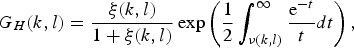 $$\eqalign{G_H(k,l) &= \displaystyle{{\xi(k,l)}\over{1+\xi(k,l)}}\exp\left(\displaystyle{{1}\over{2}}\int_{\nu(k,l)}^{\infty}\displaystyle{{{\rm e}^{-t}}\over{t}}dt\right),}$$
 $$\eqalign{\nu(k,l) &= \gamma(k,l)\xi(k,l)/(1+\xi(k,l)),}$$
where Y(k, l) is the amplitude of observed signal in the frequency domain, and G H (k, l) is the gain function. Variables ξ(k, l) and γ(k, l) are called a priori SNR and a posteriori SNR, respectively. The a posteriori SNR is defined by the current frame observation;
 $$\gamma(k,l) = \displaystyle{{\vert Y(k,l) \vert^2}\over{\sigma_m^2(k,l)}}$$
where the noise process variance
 $\sigma_{m}^{2}(k,l)$
must be obtained separately. As in [Reference Cohen and Berdugo20], we use the minima-controlled recursive averaging (MCRA) noise estimation to obtain
$\sigma_{m}^{2}(k,l)$
must be obtained separately. As in [Reference Cohen and Berdugo20], we use the minima-controlled recursive averaging (MCRA) noise estimation to obtain
 $\sigma_{m}^{2}(k,l)$
. The a priori SNR is estimated recursively using the estimated gain of the previous frame;
$\sigma_{m}^{2}(k,l)$
. The a priori SNR is estimated recursively using the estimated gain of the previous frame;
 $$\eqalign{\xi(k,l)& = c_1G_H^2(k,l-1)\gamma(k,l-1) \cr &\quad + (1-c_1) \max\{\gamma(k,l)-1, 0\}}$$
where c 1 is an adjustable weight parameter. A more detailed derivation of the above-mentioned solution could be found in [Reference Ephraim and Malah23].
OM-LSA modifies the result of LSA by taking the weighted geometric mean of G
H
(k, l) and its lower boundary
 $G_{{\rm min}}$
, where the weight is based on the speech presence probability p(k, l).
$G_{{\rm min}}$
, where the weight is based on the speech presence probability p(k, l).
 $$\eqalign{\vert \hat{X}(k,l) \vert &= G(k,l)\vert Y(k,l)\vert}$$
 $$\eqalign{G(k,l) &= [G_H(k,l)]^{p(k,l)}G_{{\rm min}}^{1-p(k,l)}. }$$
The speech presence probability is obtained by
 $$p(k,l) = \left[ {1 + \displaystyle{{q_0} \over {1 - q_0}}(1 + \xi (k,l)){\rm e}^{ - \nu (k,l)}} \right]^{ - 1}$$
where q 0 is the a priori speech absence probability.
After the noise suppression process of OM-LSA was done, there are two approaches to obtain VAD results. The first approach is to reconstruct the waveform of the noise-suppressed signal by combining the estimated amplitude
 ${\hat{X}}(k,l)$
and the original phase. Once the reconstructed waveform was obtained, any existing VAD method can be applied. The simplest example is to classify speech and non-speech frames using a power threshold, which we discuss in the next section. It is also possible to apply more sophisticated machine learning-based method, which we discuss in Section IV. The second approach is to use the speech presence probability p(k, l) defined by (10) or the likelihood ratio
${\hat{X}}(k,l)$
and the original phase. Once the reconstructed waveform was obtained, any existing VAD method can be applied. The simplest example is to classify speech and non-speech frames using a power threshold, which we discuss in the next section. It is also possible to apply more sophisticated machine learning-based method, which we discuss in Section IV. The second approach is to use the speech presence probability p(k, l) defined by (10) or the likelihood ratio
 $\Lambda(k,l)$
used in [Reference Sohn, Kim and Sung17]. They can be integrated to the framewise score as follows.
$\Lambda(k,l)$
used in [Reference Sohn, Kim and Sung17]. They can be integrated to the framewise score as follows.
 $$\eqalign{P(l) &= \prod_{k=0}^{K-1} p(k,l),}$$
 $$\eqalign{\Lambda(l) &= \prod_{k=0}^{K-1} \Lambda(k.l), \cr & = \prod_{k=0}^{K-1} \displaystyle{{1}\over{1+\xi(k,l)}}\exp \displaystyle{{\gamma(k,l)\xi(k,l)}\over{1+\xi(k,l)}}}$$
where K is the number of frequency components. VAD can be realized simply by applying a threshold for these framewise scores.
B) Augmented implementation of OM-LSA
The original OM-LSA estimator was intended to provide better speech signal for communication and recognition. Therefore, it was designed to maintain the balance between lowering the noise level and not causing the distortion. However, reducing the noise is particularly important for VAD, while the distortion is rarely harmful. In view of the priority of noise removal, we propose to use some augmentation techniques for the OM-LSA speech estimator.
The first step of augmentation focuses on (6). Although MCRA is known to be a reliable noise estimation algorithm, we believe that the noise level must be over-estimated so that any unreliable part of the spectrogram does not affect the VAD results. In fact, we formerly found that the noise level must be under-estimated to obtain more accurate results of speech recognition [Reference Obuchi, Takeda and Togami24], because distortion is the main cause of misrecognition. Both under and over estimation of the noise can be realized by introducing a weight factor α as follows.
 $$\gamma(k,l) = \displaystyle{{\vert Y(k,l)\vert^2}\over{\alpha\sigma_m^2(k,l)}}.$$
The second step of augmentation focuses on (8) that defines how the estimated gain is applied to the speech amplitude. Augmentation is realized simply by introducing a modification parameter β as follows.
 $$ \vert \hat{X}(k,l)\vert =G^{\beta}(k,l)\vert Y(k,l) \vert.$$
The third step of augmentation is a screening step of the prominent noise component. In contrast that speech has a wideband spectrum, there are kinds of noises that have a very sharp peak in the power spectrum, such as electrical beeps and musical instrument sounds. The prominent component in the power spectrum could be removed by the process described as follows.
 $$ \vert \hat X(k,l)\vert = \left\{ {\matrix{ {G^\beta (k,l)\vert Y(k,l)\vert} & {{\rm rank}(k) \ge \eta K} \cr 0 \hfill & {{\rm otherwise},} \hfill \cr } } \right.$$
where rank(k) is the number of frequency components whose magnitude is larger than the kth frequency. At last, our VAD-oriented OM-LSA-based speech estimator is defined by equations (4), (5), (7), (9), (10), (13), and (15).
III. CLASSIFICATION WITHOUT MODEL TRAINING
After the noise suppressed signal is obtained, we extract framewise features and classify each frame into speech or non-speech. The simplest classification algorithm is to apply a threshold to the frame power, which is calculated as follows.
 $$ Q(l)=\sum_{k=0}^{K-1}w(k)\vert \hat{X}(k,l)\vert^2$$
where w(k) is the A-weighted filter coefficient corresponding to the kth frequency. In the above equation,
 ${\hat{X}}(k,l)$
is not necessarily the same as that of (15) because sometimes the optimal time scale is not equal between noise suppression and VAD. In this paper, the frame power for VAD is calculated using 20 ms half-overlapping frames from the reconstructed waveform, whereas the noise suppression was executed using 32 ms half-overlapping frames. In fact, we apply the modification from (14) to (15) not directly during noise suppression. Instead, we apply (15) for the reconstructed waveform.
${\hat{X}}(k,l)$
is not necessarily the same as that of (15) because sometimes the optimal time scale is not equal between noise suppression and VAD. In this paper, the frame power for VAD is calculated using 20 ms half-overlapping frames from the reconstructed waveform, whereas the noise suppression was executed using 32 ms half-overlapping frames. In fact, we apply the modification from (14) to (15) not directly during noise suppression. Instead, we apply (15) for the reconstructed waveform.
Once the frame power is calculated, the frame is labeled as speech if the power is larger than the threshold. Although this approach is not effective in low-SNR environments by itself, it works quite effectively when it is combined with noise suppression. It should be also noted that the same principle is applicable to other framewise features, such as P(l) and Λ(l).
A typical modification of the threshold-based VAD is to add inter-frame smoothing. Consonants at the beginning and the end of an utterance is likely to be mislabeled as non-speech due to its small power. Therefore, it is reasonable to add several-frame speech periods (hangovers) on both ends of the period labeled as speech. It is also reasonable to remove (relabel as non-speech) very short speech periods because they are likely to be transient noise, and to fill (relabel as speech) short non-speech periods because they are likely to be voiceless intervals within utterances.
Throughout this paper, we remove speech periods of 100 ms or shorter, fill non-speech periods of 80 ms or shorter, and add 80 ms hangovers on both ends of the speech period.
IV. CLASSIFICATION WITH UNSUPERVISED AND SUPERVISED MODEL TRAINING
If we use multi-dimensional features, more accurate VAD results could be obtained using more sophisticated classifiers. Such classifiers are mostly model-based, so we need to prepare a set of training data.
If we have a set of unlabeled training data, then the training process is called unsupervised. Clustering such as k-means algorithm is an example of unsupervised training. In the case of VAD, two clusters corresponding to the speech class and non-speech class are generated. The training process itself cannot decide which cluster corresponds to the speech, but the non-speech cluster can be easily found by testing a silent frame.
If we have a set of correctly labeled training data, then we can train the classifier model more precisely. It is called supervised training. In this paper, we investigate three model-based supervised classifiers: decision tree (DT), SVM, and CNN.
For all clusterers and classifiers, the same feature set is used. The feature vector for the lth frame consists of
 $\vert \hat{X}(k,s)\vert^{2}$
, where 0 ≤ k < K and
$\vert \hat{X}(k,s)\vert^{2}$
, where 0 ≤ k < K and
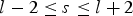 $l-2 \leq s \leq l+2$
. The resulting feature vector has 5K elements. In the rest of this paper, K = 40 is used.
$l-2 \leq s \leq l+2$
. The resulting feature vector has 5K elements. In the rest of this paper, K = 40 is used.
When we use the model-based classifier, we omit the modification by (15), and use (14) instead. It is because the modification from (14) to (15) is learnable by the classifier if it improves the classification accuracy for the training data. Moreover, the machine learning algorithm may find even a better modification.
When we use the framewise clusterers (k-means) and framewise classifiers (DT, SVM, and CNN), inter-frame smoothing is applied as in the case of simple thresholding. Additional 40 ms speech periods were added on both ends of the utterance. Other criteria are the same as in the case of simple thresholding; noises of 100 ms or shorter were removed and silences of 80 ms or shorter were filled.
V. EXPERIMENTAL RESULTS
A) CENSREC-1-C evaluation framework
The proposed VAD algorithm was evaluated using CENSREC-1-C [Reference Kitaoka25], a public VAD evaluation framework. The data part of CENSREC-1-C consists of two datasets: simulated dataset and real dataset. In this paper, we used the real dataset made of Japanese connected digit utterances. The CENSREC-1-C real dataset is further divided into four subsets based on the environment (university restaurant and vicinity of highway street) and SNR level (high and low). Its details are shown in Table 1, where the average noise levels were cited from [Reference Kitaoka25] and the SNR levels were estimated using WADA-SNR [Reference Kim and Stern26].
Table 1. Detail of CENSREC-1-C real dataset.

CENSREC-1-C includes not only the data themselves, but also the voice activity labels and performance calculation tools. When a specific algorithm and corresponding settings are given, the false alarm rate (FAR) and the false rejection rate (FRR) are automatically calculated. FAR is the ratio of incorrectly labeled non-speech frames over the total non-speech frames. FRR is the ratio of incorrectly labeled speech frames over the total speech frames. We also use the average error rate (AER), which is the average of FAR and FRR.
B) Evaluation using classifiers without model training
The first set of experiments using CENSREC-1-C was conducted to compare three framewise scores, P(l), Λ(l), and Q(l). The threshold-based classifier was applied to those three scores obtained by statistical noise suppression without augmentation (
 $\alpha=1.0, \beta=1.0, \eta=0.0$
). Other parameter setting was the same as in [Reference Obuchi, Takeda and Kanda21] (
$\alpha=1.0, \beta=1.0, \eta=0.0$
). Other parameter setting was the same as in [Reference Obuchi, Takeda and Kanda21] (
 $C_{1}=0.99, G_{{min}}=0.01, q_{0}=0.2$
). Figure 1 shows the ROC curves obtained by applying various threshold values. Since CENSREC-1-C provides the baseline VAD tool, the corresponding ROC curve was plotted for comparison. It is clear that all three scores resulted in lower FARs and FRRs than the baseline. Among them, P(l) is clearly less effective, and Q(l) is slightly better than Λ(l). Accordingly, Q(l) is used as the framewise score in this section.
$C_{1}=0.99, G_{{min}}=0.01, q_{0}=0.2$
). Figure 1 shows the ROC curves obtained by applying various threshold values. Since CENSREC-1-C provides the baseline VAD tool, the corresponding ROC curve was plotted for comparison. It is clear that all three scores resulted in lower FARs and FRRs than the baseline. Among them, P(l) is clearly less effective, and Q(l) is slightly better than Λ(l). Accordingly, Q(l) is used as the framewise score in this section.

Fig. 1. Comparison of framewise scores. The same threshold-based classifier was applied.
The second set of experiments was to confirm the effectiveness of the augmented statistical noise suppression. The same threshold-based classifier was applied to the output of statistical noise suppression, in which various augmentation was applied.
Figure 2 shows the effectiveness of noise over-estimation, defined by (13). The values of β and η were not augmented, and the value of α was changed. The point α = 1.0 corresponds to the original OM-LSA, and it was reported that
 $\alpha\approx 0.2$
is optimal for speech recognition [Reference Obuchi, Takeda and Togami24]. For each value of α, various thresholds were tested,
$\alpha\approx 0.2$
is optimal for speech recognition [Reference Obuchi, Takeda and Togami24]. For each value of α, various thresholds were tested,
 ${\rm AER}=({\rm FAR}+{\rm FRR})/2$
was calculated, and the smallest AER was plotted. The results revealed that decreasing the value of α is only harmful for VAD, and AER drops rapidly when α increases from 1.0 to 2.0. When α is further increased, AER seems to be saturated.
${\rm AER}=({\rm FAR}+{\rm FRR})/2$
was calculated, and the smallest AER was plotted. The results revealed that decreasing the value of α is only harmful for VAD, and AER drops rapidly when α increases from 1.0 to 2.0. When α is further increased, AER seems to be saturated.

Fig. 2. Effect of over-subtraction expressed by various α.
Figure 3 shows the effectiveness of gain nonlinearity, defined by (14). The value of α was fixed at 5.0, and various values of β were tried. In this case, some improvements were observed with increasing β, but it is not as dramatic as in the case of increasing α.

Fig. 3. Effect of gain augmentation expressed by various β.
The results obtained by various values of η are shown in Fig. 4, where β was fixed at 1.4. Again, AER drops rapidly with increasing η, and reached its smallest value at η = 0.07. The best AER was 9.93%, where
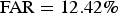 ${\rm FAR}=12.42\%$
and
${\rm FAR}=12.42\%$
and
 ${\rm FRR}=7.43\%$
.
${\rm FRR}=7.43\%$
.

Fig. 4. Effect of prominent component removal expressed by various η.
We also investigated the possibility of using adaptive parameters. Obviously, the most effective parameter is the frame power threshold. Since the dataset of CENSREC-1-C is made of four subsets, we checked the AER of our best setting (
 $\alpha=5.0, \beta=1.4, \eta=0.07$
) obtained with the optimal threshold for each subset. In this case, the AERs for Restaurant (SNR high), Restaurant (SNR low), Street (SNR high), and Street (SNR low) were 7.00, 18.03, 2.73, and 3.94% respectively. The average was 7.93%, which is much better than the AER obtained with the fixed threshold (9.93%).
$\alpha=5.0, \beta=1.4, \eta=0.07$
) obtained with the optimal threshold for each subset. In this case, the AERs for Restaurant (SNR high), Restaurant (SNR low), Street (SNR high), and Street (SNR low) were 7.00, 18.03, 2.73, and 3.94% respectively. The average was 7.93%, which is much better than the AER obtained with the fixed threshold (9.93%).
Similar experiments were conducted with the adaptive α, β, and η. In the case of α (see Fig. 2), the lowest AER of 10.44% was still improved to 9.27%. In the case of β (see Fig. 3), the lowest AER of 10.35% was still improved to 9.53%. Finally, in the case of η (see Fig. 4), the lowest AER of 9.93% was improved to 9.37%.
Although these results indicate the potential value of adaptive parameters, their effectiveness are strongly dependent on the correct evaluation of the environment. We must consider the risk of performance degradation caused by the incorrect parameter setting.
C) Classifier training
More accurate VAD results could be achieved by the model-based classifiers. In this paper, we investigate three types of model-based classifiers: DT, SVM, and CNN. We also try k-means clustering to compare supervised and unsupervised training. Before applying them to CENSREC-1-C, we train the classifiers and clusterer using a separate dataset.
1) Training and development data
The dataset for classifier and clusterer training, referred to as Noisy UT-ML-JPN database in this paper, was created using UT-ML public database [27] and our proprietary noise data. The noise data were recorded in a running car and in a cafeteria; they were added to the utterances of Japanese subset of UT-ML database with SNR of 0, 5, and 10 dB. Speech/non-speech labels for Noisy UT-ML-JPN database were generated automatically by applying a power threshold for the clean version of UT-ML database. The labeling process is completely framewise, meaning that inter-frame smoothing was not applied.
The Japanese subset of UT-ML database includes six male and six female speakers, each of which read one long article (54.8 s on average) and 50 short phrases (3.3 s on average). Original data were recorded by 16 kHz sampling rate, but they were downsampled to 8 kHz. One second silences were appended on both ends of utterances before noises were added.
After adding the noise, augmented statistical noise suppression described in Section II-B) was applied. Based on the results of Section V-B) and [Reference Obuchi, Takeda and Kanda21]Footnote 1 , the parameter setting was α = 5.0, β = 1.4, and η = 0.07. Applying the same noise suppression process to the training and test data are called noise adaptive training (NAT), and known to be effective for speech recognition [Reference Deng, Acero, Plumpe and Huang28]. We also prepare the clean version of the training data for comparison.
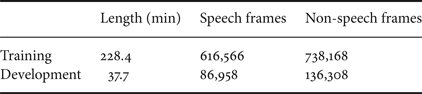
Finally, data of one male and one female speakers were used for development, and the other data were used for model training. The size of the training and development set are shown in Table 2.
Table 2. Length and number of frames of Noisy UT-ML-JPN database.
2) Toolkits
The classifiers were trained using publicly available toolkits. WEKA [Reference Hall, Frank, Holmes, Pfahringer, Reutemann and Witten29] was used for DT and SVM training, and Caffe [Reference Jia30] was used for CNN training. The k-means clustering program was prepared by ourselves.
When we use WEKA for DT and SVM, we adopt the classifier ensemble approach. Although we have plenty of training samples (more than 600 k of speech and more than 700 k of non-speech), it takes too long to execute the training using the whole data at once. Therefore, we split the training data into small chunks, and trained many classifiers using different data chunks. The final classification result can be obtained by voting of these small classifiers. CNN training and k-means clustering were executed using all data.
DT by WEKA (J48) runs without any specific parameter adjustment. SVM by WEKA (SMO) requires at least selection of the kernel, so we used the two-dimensional polynominal kernel. CNN by Caffe requires quite a few parameters to be set, but we only show the network topology in Fig. 5, that would be the most important information.

Fig. 5. CNN topology. Relu stands for rectified linear unit. The output layer (ip2) has two units corresponding to speech and non-speech.
3) Preliminary evaluation
Before going back to CENSREC-1-C, we checked the basic performance of three classifiers and one clusterer using the development data. The development data were processed by augmented statistical noise suppression using the same parameters as the training data. The processed data were then divided into frames and classified by either DT, SVM, CNN or k-means.
Figure 6 depicts the results obtained by the classifier ensemble of DT and SVM with various sizes. Inter-frame smoothing was not applied, so the graph shows the pure performance of framewise classification. It should also be noted that the classifier directly classifies the frame data, so we obtain a single pair of FAR and FRR instead of the ROC curve. The results indicated that SVM is superior to DT if only few classifiers were used. However, it was reversed if we have seven or more classifiers. AER was saturated at about 20 classifiers (SVM) or 40 classifiers (DT).

Fig. 6. Preliminary evaluation of classifier ensemble.
Figure 7 shows the comparison of simple thresholding, k-means clustering, and various classifiers. If we apply simple thresholding, AER was 21.29%. In the case of k-means clustering, an additional bias θ was introduced to play the role of adjustable threshold. A frame is labeled as non-speech if
 $d_{ns}-d_{s}<\theta$
, where d
s
(d
ns
) is the distance between the frame and the centroid of speech (non-speech) cluster. Although AER was as high as 27.19% when θ = 0, it becomes 20.44% if the value of θ was optimized. The AERs of DT and SVM were clearly better than simple thresholding and k-means. On the right-hand side of the figure, AERs obtained by various CNNs are plotted, where L is the number of fully-connected intermediate layers (rectangular block including ip1+relu1 of Fig. 5). As we expected, CNN (NAT) provides better results than CNN (clean), indicating that NAT was effective. It is also found that the deeper the network is, the more accurate classification results were obtained.
$d_{ns}-d_{s}<\theta$
, where d
s
(d
ns
) is the distance between the frame and the centroid of speech (non-speech) cluster. Although AER was as high as 27.19% when θ = 0, it becomes 20.44% if the value of θ was optimized. The AERs of DT and SVM were clearly better than simple thresholding and k-means. On the right-hand side of the figure, AERs obtained by various CNNs are plotted, where L is the number of fully-connected intermediate layers (rectangular block including ip1+relu1 of Fig. 5). As we expected, CNN (NAT) provides better results than CNN (clean), indicating that NAT was effective. It is also found that the deeper the network is, the more accurate classification results were obtained.

Fig. 7. Preliminary evaluation by comparing various classifiers.
D) Evaluation using model-based classifiers
Finally, we applied various classifiers to CENSREC-1-C. The evaluation procedure was the same as in the preliminary evaluation, except that inter-frame smoothing was applied. In addition, a gain adjustment factor was multiplied to to input signal before applying DT, SVM, and CNN, in order to compensate the unmatched data acquisition environment. The gain factor plays the role similar to the adjustable threshold; a large gain factor is equivalent to a small threshold, and vice versa. Therefore, we can obtain an ROC curve by using various gain factors. The bias of k-means clustering also serves to make an ROC curve.
Figure 8 shows the ROC curves obtained by k-menas, DT, SVM, and CNNs with various number of intermediate layers. The results of threshold-based classifier, which is exactly the same as η = 0.07 of Fig. 4, was added for comparison. It is clear that the model-based classifiers achieved better results than the threshold-based classifier. However, unsupervised training by k-means clustering did not improve the accuracy. As for CNNs, unlike the preliminary evaluation, the shallowest network achieved the most accurate VAD results. The different tendency regarding to the number of layers can be attributed to the overfitting effect. In the preliminary evaluation, the deeper CNN can learn even small details of the training data which can contribute only under the matched condition. In the CENSREC-1-C evaluation, the shallower CNN has a more generalized model, which contributes to avoid errors related to the condition-specific features. That argument is supported by the fact that the superiority of DT over SVM is not observed in the CENSREC-1-C evaluation, because DT is more likely to overfit the training data even though it includes some pruning algorithms.

Fig. 8. ROC curves for CENSREC-1-C obtained by various classifiers. DT and SVM represent the voting results of 100 classifiers.
So far, we have found that the combination of augmented statistical noise suppression and CNN-based classifier achieved the best VAD accuracy among considered algorithms. In Fig. 9, it is demonstrated how the ROC curve shifted toward the left-bottom corner. SNS-thres, which is the copy of Q(l) of Fig. 1, is our starting point, and it was greatly improved by augmented statistical noise suppression, resulted in ASNS-thres. There was some additional improvement by introducing CNN, and the final ROC curve was plotted as ASNS-CNN. We also plotted some published results using CENSREC-1-C, such as using CRF [Reference Saito, Nankaku, Lee and Tokuda16], SKF [Reference Fujimoto and Ishizuka19], and SKF with Gaussian pruning (SKF/GP) [Reference Fujimoto, Watanabe and Nakatani31], and confirmed that the proposed algorithm outperformed them.

Fig. 9. ROC curves for CENSREC-1-C obtained by the proposed algorithms. Reference points of CRF, SKF, and SKF/GP were cited from the published papers.
Following the convention of CENEREC-1-C, the details of the VAD results obtained by ASNS-CNN are show in Fig. 10.

Fig. 10. Detail of CENSREC-1-C evaluation.
E) Computational complexity
In addition to the VAD accuracy, we confirmed the processing time and latency of the proposed algorithm. Table 3 shows the processing time for the 144 files of CENSREC-1-C dataset (6465.33 s). The noise suppression and classification programs were implemented separately on Ubuntu 16.04 running on Intel Core i7 processor (3.6 GHz) with 16 GB RAM. Although the programs were not optimized in terms of speed, the real-time factor (RTF) was 0.051, meaning that the total processing time was about 1/20 of the real time.
Table 3. Processing Time for CENSREC-1-C.

Regardless of the processing speed, the proposed algorithm cannot avoid the framing latency. Noise suppression causes a half-frame (16 ms) latency and VAD causes five half-overlapping frame latency (60 ms). The total latency up to 84 ms (including 8 ms frame boundary adjustment) is not negligible, but the speech recognition system uses similar number of successive frames as the input feature. Therefore, the latency does not matter if the proposed VAD algorithm is used for speech recognition.
VI. CONCLUSIONS
In this paper, we analyzed state-of-the-art VAD algorithms from the perspective of statistical noise suppression and framewise speech/non-speech classification. Based on the analysis, we proposed two modification approaches. First, statistical noise suppression was augmented using additional parameters so that all the unreliable spectral components were removed. Second, CNN-based classifier was introduced to improve the accuracy of the framewise classifier. Evaluation experiments using the CENSREC-1-C public framework demonstrated that each of the modifications achieved noticeable improvements in VAD accuracy. The results of the proposed algorithm were also compared with results reported in the literature, indicating that the proposed algorithm is better than SKF/GP, which was shown in [Reference Fujimoto, Watanabe and Nakatani31] to be superior to the standard VAD algorithms such as ITU-T Recommendation G.729 Annex B [32], ETSI Advanced Front-End [33], and Sohn's algorithm [Reference Sohn, Kim and Sung17].
A comparison between matched and unmatched conditions indicated that it is important to avoid overfitting problem under unmatched conditions; hence a relatively shallow CNN is appropriate in general. The effect of the overfitting problem would also be related to the size and variety of the training data; however, this remains an open problem for future study.
Yasunari Obuchi received B. S. and M. S. degrees in Physics from the University of Tokyo in 1988 and 1990, respectively. He received Ph.D. in Information Science and technology from the University of Tokyo in 2006. From 1992 to 2015, he had been with Central Research Laboratory and Advanced Research Laboratory, Hitachi, Ltd. From 2002 to 2003, he was a visiting scholar at Language Technologies Institute, Carnegie Mellon University. He was a visiting researcher at Information Technology Research Organization, Waseda University from 2005 to 2010. He also worked at Clarion Co., Ltd. from 2013 to 2015. Since 2015, he has been a Professor at School of Media Science, Tokyo University of Technology. He was a co-recipient of the Technology Development Award of the Acoustical Society of Japan in 2000. He is a member of IEEE, Information Processing Society of Japan, Institute of Electronics, Information and Communication Engineers, Acoustical Society of Japan, and Society for Art and Science.


 Open access