


1. Introduction
The understanding of the laminar-to-turbulent transition process on swept wings is a crucial issue both from a theoretical and practical point of view for aerodynamic optimization and transition control. This is why, over the last decades, many studies have been conducted to better understand this phenomenon. When the environmental disturbances have a sufficiently small amplitude, as often occurs in flight conditions, instabilities growing following a linear mechanism can develop within the boundary layer. It is then important to identify the physical mechanism involved and the spatial structure of the instability in order to control it and thus delay the transition. In the case of swept wings, and in the absence of contamination by the turbulence of the fuselage, three types of instabilities are mainly responsible for the transition: attachment-line (AL); cross-flow (CF); and Tollmien–Schlichting (TS) instabilities.
The TS instability is related to the streamwise component of the flow and takes the form of vortices almost perpendicular to the streamwise direction. As mentioned by Reed & Saric (Reference Reed and Saric1989), TS instabilities are destabilized by an adverse pressure gradient and arise in regions with no or weak positive pressure gradient. In the case of a Blasius boundary layer flow, the value of the critical Reynolds number based on the free stream velocity and the boundary layer displacement thickness is  $Re_{crit}=520$ and the phase speed of the corresponding marginal mode is $0.397$ (Schmid & Henningson Reference Schmid and Henningson2001).
Attachment-line instabilities are characterized by counter-rotating vortices developing in the attachment line region and aligned with the chordwise direction. The mechanism responsible for these instabilities is similar to that of the two-dimensional (2-D) TS instabilities in the  $(z,\eta )$ plane, where $z$ and $\eta$ are, respectively, the spanwise and wall-normal directions. This instability has long been studied through the analysis of a flow impinging on a flat swept plate with the chordwise velocity linear in the chordwise coordinate $x$, representative of the attachment line of a swept cylinder. This model is called the swept Hiemenz flow (SHF) and was comprehensively studied in Hall, Malik & Poll (Reference Hall, Malik and Poll1984) where Görtler–Hammerlin perturbations with a linear dependency in the chordwise direction cause the flow to be linearly unstable above a critical sweep Reynolds number $Re_S=583$. The sweep Reynolds number $Re_S$, based on the spanwise velocity and a typical length scale of the boundary layer at the attachment line, is commonly used in studies dealing with attachment line flows. In order to remove the assumption about chordwise linear dependency of the perturbation, Lin & Malik (Reference Lin and Malik1996) considered more general 2-D perturbations. They validated the threshold value of Hall et al. (Reference Hall, Malik and Poll1984) and noted the observation of symmetric and antisymmetric modes, the symmetric Görtler–Hammerlin mode described by Hall et al. (Reference Hall, Malik and Poll1984) remaining the most unstable. Following on from this study, Lin & Malik (Reference Lin and Malik1997) studied the influence of leading-edge curvature using second-order boundary-layer theory, which made it possible to show the stabilizing effect of leading-edge curvature on AL instabilities.
Unlike AL and TS instabilities, CF instabilities are inflectional and are caused by the combined effect of sweep and wall curvature farther downstream. Indeed, the centripetal force and the favourable pressure gradient create a deflection of the flow outside the boundary layer. Within the boundary layer, the centripetal force decreases while the pressure gradient is conserved, creating a velocity profile with an inflection point, which is the source of CF instability. As described in the review by Saric, Reed & White (Reference Saric, Reed and White2003), CF instability can be either steady or travelling. It is characterized by corotating vortices almost aligned with the streamwise direction, especially for the steady modes. Contrary to the TS instabilities, CF instabilities are often destabilized by a negative pressure gradient. They are sufficiently strong (inviscid instability) to trigger absolute instability in the chordwise direction, see Lingwood (Reference Lingwood1997).
During the 20th century, all these instabilities were mainly studied independently from simplified models with assumptions on the flow or a perturbation form depending on the type of instability sought. However, the origin of this independence mostly comes from practical limitations rather than physical considerations and a realistic instability may be a superposition of different types. By investigating the interaction of oblique waves with 2-D waves for the SHF case, Hall & Seddougui (Reference Hall and Seddougui1990) suggested a connection between AL and CF instabilities. Then, Bertolotti (Reference Bertolotti2000) found modes connecting AL to CF in the SHF case using confluent hypergeometric functions. To study the diversity of the instabilities, the need to perform stability analyses which are global in the chordwise direction on domains that extend over the whole leading edge was perceived. These chordwise-global analyses, contrary to chordwise-local analyses, allow us to directly conclude on the absolute nature of the instability in the chordwise direction (Huerre & Monkewitz Reference Huerre and Monkewitz1990) but also to have access to its wavemaker, as well as to its whole spatial structure. The concept of wavemaker was introduced by Gianetti & Luchini (Reference Gianetti and Luchini2007) and is relevant for the identification of the physical mechanisms at play. The increase of computational capacities has made this type of global analysis possible, but the difficulty lies in the possibly very high sensitivity of the computed eigenvalues to numerical parameters such as domain size or eigenvalue shift (Alizard & Robinet Reference Alizard and Robinet2007; Garnaud et al. Reference Garnaud, Lesshafft, Schmid and Huerre2013; Brynjell-Rahkola et al. Reference Brynjell-Rahkola, Shahriari, Schlatter, Hanifi and Henningson2017). Cerqueira & Sipp (Reference Cerqueira and Sipp2014) have shown that this issue is linked to the modification of the  $\epsilon$-pseudospectrum with the extension of the domain. To date, only a few studies deal with chordwise-global stability analyses using a domain covering the entire leading edge (Mack, Schmid & Sesterhenn Reference Mack, Schmid and Sesterhenn2008; Mack & Schmid Reference Mack and Schmid2011; Meneghello, Schmid & Huerre Reference Meneghello, Schmid and Huerre2015). In Mack et al. (Reference Mack, Schmid and Sesterhenn2008), a first temporal chordwise-global stability analysis was conducted on a parabolic leading-edge in supersonic flow. The authors reported ‘connected modes’ with features of both AL and CF. In Mack & Schmid (Reference Mack and Schmid2011), a neutral curve was established, still in supersonic condition. Their study was done at a constant sweep angle, which implies a simultaneous variation of the sweep and leading-edge Reynolds numbers $Re_S$ and $Re_R$. Meneghello et al. (Reference Meneghello, Schmid and Huerre2015) dealt with the incompressible flow around the leading-edge of a Joukowski airfoil. Only strongly stable modes were analysed. One of their observations is the appearance of an AL/CF connected mode with a first spatial growth of the direct mode close to the attachment line and a second spatial amplification farther downstream, where the direct mode has characteristics reminiscent of a CF type instability. They used the wavemaker to conclude that the observed mode is fed by the AL instability. This last result additionally implied that effective open-loop control strategies should focus on baseflow modifications in the region where the AL instability prevails. Thus, chordwise-global analyses provide important information about the spatial structure of the modes and their sensitivity, and the previous studies of leading-edge instabilities have highlighted the complexity of the modes involved. Yet, only a strongly stable configuration around a Joukowski profile has been studied for the case of an incompressible flow and studies of unstable or marginally stable flows have been limited to a narrow field of the parameter space in a compressible case around a parabolic body.
The first objective of this paper is to extend the study of boundary layer instabilities that develop in an incompressible flow around the leading-edge of swept realistic airfoils, here the ONERA-D and Joukowski airfoils with infinite span. In particular, we are interested in studying the neutral curves in extended parameter space and in characterizing the physical nature of the chordwise-global modes along them. By studying in depth the features of the marginal modes, including the study of the wavemaker position, we would like to further the study of the diversity of the modes developing on the leading-edge and improve our understanding of the connection between the different types of instabilities. We also want to investigate the impact of the streamwise pressure gradient on the instabilities by comparing the results between a ONERA-D airfoil and a Joukowski airfoil, which exhibit strongly different pressure gradients.
The chordwise-global analyses used in our study remain local in the spanwise direction. Therefore, the convective or absolute nature in the spanwise direction of the studied instabilities is still to be explored. This problem aims at determining whether an instability in the flow has a chance to sustain the perturbation so as to grow temporally at a given spanwise position and contaminate the whole airfoil, or whether it will be convected away along the span. Studies addressing this issue were conducted at the end of the 20th century. Indeed, Türkylmazoglu & Gajjar (Reference Türkylmazoglu and Gajjar1999) and Lingwood (Reference Lingwood1997), respectively, dealt with the incompressible SHF and Falkner–Skan–Cooke boundary layer and found that they are absolutely unstable in the chordwise direction, but may still be only convectively unstable in the spanwise direction. Taylor & Peake have also been interested in this problem for genuine airfoils in incompressible (Taylor & Peake Reference Taylor and Peake1998) and compressible (Taylor & Peake Reference Taylor and Peake1999) regimes. In both cases, they also found convectively unstable flows without absolute instabilities in both streamwise and CF directions. Similarly, (Piot & Casalis Reference Piot and Casalis2009) studied the absolute instability mechanisms on a swept cylinder with imposed spanwise periodic conditions. All previously mentioned absolute stability analyses were conducted using stability analyses that are local both in the spanwise and chordwise directions.
The second objective of this paper is to study the absolute/convective nature in the spanwise direction of the instabilities developing in the boundary layer of the incompressible flow around the leading-edge of the ONERA-D airfoil. To the authors’ knowledge, this is the first study of this nature using chordwise-global stability analyses.
The outline of the paper is the following. In § 2 the methodology that will be used in this paper is described. The flow configurations as well as the governing equations and the computational domain are introduced. The numerical methods and the procedure for finding modes with zero-group velocity are also detailed. In § 3 the results and discussions are presented. In § 3.1, some results of the baseflow are described. In § 3.2, a neutral curve for the swept ONERA-D airfoil is drawn and a detailed analysis of its structure and its marginal modes is provided. The convective/absolute nature of the instabilities is tackled in § 3.3. Then, a parametric study of the influence of  $Re_R$ is performed by comparing neutral curves in the case of the ONERA-D in § 3.4. Finally, in § 3.5, the neutral curves for the swept ONERA-D and Joukowski airfoils are compared with assess the influence of the airfoil shape.
2. Methodology
2.1. Flow configurations
We consider the swept ONERA-D and Joukowski airfoils of infinite span at  $0^\circ$ angle of attack, the Joukowski airfoil having a thickness parameter $\epsilon =0.1$. The ONERA-D is a reference airfoil for the study of the boundary layer transition and has a shape designed specifically to stabilize TS waves. We pick an orthonormal coordinate system $(x,y,z)$ whose origin is located on the leading-edge, the $x$ direction being along the chord orthogonal to the leading-edge, the $z$ direction along the span and the $y$ direction orthogonal to the symmetry plane (see figure 1).

Figure 1. (a) Schematic of the mesh and flow configuration with the ONERA-D airfoil. (b) Angles and coordinate systems are indicated. An external streamline is illustrated in green. The blue lines correspond to the leading/trailing edges.
The leading-edge radius of curvature of the airfoils in the  $(x,y)$ plane is noted $r_c$ and the sweep angle $\varLambda =\textrm {angle}(\boldsymbol {U}^\infty, \boldsymbol {x})$ with the inflow velocity $U^\infty$ which may be decomposed as a sweep velocity $U_z^\infty =U^\infty \sin \varLambda$ and a chordwise velocity $U_x^\infty =U^\infty \cos \varLambda$ (with $U_y^{\infty }=0$). The chord in the direction of the free stream velocity is noted $C$, while $C_n= C \cos \varLambda$ is the chord normal to the leading-edge of the airfoil.
We will consider two local orthonormal coordinate systems:
(i) $(s,\eta,z)$, where $s$ is the curvilinear abscissa along the surface of the airfoil in a $(z=cst)$ plane and $\eta$ is the wall-normal direction ($\eta =0$ corresponds to the surface);
(ii)
$(\chi,\eta,b)$, where $\chi$ is a curvilinear abscissa along a streamline of the external baseflow velocity field, just outside of the boundary layer (see § 3.1) – again $\eta$ is the wall-normal direction and $b$ is normal to the plane $(\chi,\eta )$.


Two non-dimensional parameters are needed to describe the flow configuration. A natural parameterization is the one based on the sweep angle and the streamwise Reynolds number,
 \begin{equation} \left( \varLambda, \ Re_Q=\frac{U^\infty C}{\nu} \right), \end{equation}
where  $\nu$ denotes the kinematic viscosity. These two parameters, commonly used in wind tunnel experiments, will be used in the result § 3.5 to compare the stability of the Joukowski and ONERA-D airfoils.
In our study, we will mainly use a parameterization more representative of the physics of the flow at the leading-edge by defining the ‘leading-edge Reynolds number’  $Re_R$ and the ‘sweep Reynolds number’ $Re_S$:
 \begin{equation} \left( Re_R=\frac{U_x^\infty r_c}{\nu}, \ Re_S=\frac{U_z^\infty \varDelta}{\nu} \right). \end{equation}
Here  $\varDelta$ is a typical length scale of the boundary layer thickness at the attachment line and is based on the potential flow,
 \begin{equation} \varDelta = \sqrt{\frac{\nu}{S_0}}, \quad S_0=\left. \frac{\partial U_s^{pot}}{\partial s}\right|_{x=0,y=0}, \end{equation}
where  $U_s^{pot}$ denotes the $s$-component of the potential velocity. The detail of the calculation of the potential flow will be given in § 2.2.1. Here $S_0$ is then the strain rate of the potential flow around the profile at the AL.
This parameterization has been used intensively in the study of transition in simplified leading-edge configurations. The sweep Reynolds number  $Re_S$, often used for the study of attachment line flows, and sometimes also denoted $\bar {R}$, drives the instability mechanism along the attachment line (Hall et al. Reference Hall, Malik and Poll1984; Lin & Malik Reference Lin and Malik1996). The leading-edge Reynolds number $Re_R$ can be seen as a scaling of the boundary layer thickness with respect to the radius of curvature at the AL since
 \begin{equation} \frac{\varDelta}{r_c}=\frac{1}{\sqrt{K \,Re_R}}, \end{equation}
where  $K=S_0 r_c / U_x^\infty$.
Lin & Malik (Reference Lin and Malik1997) used this Reynolds number to measure the influence of the leading-edge curvature on the AL instabilities. Here  $K$ is the ratio between two length scales: the leading-edge radius of curvature $r_c$ and the characteristic length scale $U_x^\infty /S_0$ of variation of the potential flow in the vicinity of the leading edge.
For the ONERA-D and Joukowski airfoils, we have  $(r_c/C_n,K) = (0.0180,1.37484)$ and $(r_c/C_n,K) = (0.016129,1.2669)$, respectively (for comparison, $(r_c/C_n,K) = (0.5,2)$ in the case of the cylinder).
Both sets of parameters  $(Re_Q,\varLambda )$ and $(Re_R,Re_S)$ may be linked through
 \begin{equation} \left( \tan \varLambda=\sqrt{\frac{K}{Re_R}}Re_S, Re_Q=Re_R\frac{1+\tan^2 \varLambda}{r_c/C_n} \right). \end{equation}
2.2. Governing equations and computational domain
In the context of our study, we seek to determine the stability of a perturbation  $\boldsymbol {q}(x,y,z,t)=(\boldsymbol {u},p)(x,y,z,t)$ of small amplitude which emerges within a baseflow $\boldsymbol {Q}(x,y,z,t)=(\boldsymbol {U},P)(x,y,z,t)$. The baseflow being steady and homogeneous in $z$, then we simply have $\boldsymbol {Q}(x,y,z,t)=\boldsymbol {Q}(x,y)$.
The total flow  $\boldsymbol {Q}_{tot}$ is expressed as the sum of the baseflow and the perturbation,
 \begin{equation} \boldsymbol{Q}_{tot}(x,y,z,t)=\boldsymbol{Q}(x,y)+\epsilon\boldsymbol{q}(x,y,z,t), \end{equation}
with  $\epsilon \ll 1$.
We want to study the temporal stability of the perturbations by expressing them in the form  $\boldsymbol {q}(x,y,z,t)=\tilde {\boldsymbol {q}}(x,y,z){\rm e}^{-{\rm i}\omega t}$ with $\omega \in \mathbb {C}$. The real part $\omega _r$ and imaginary part $\omega _i$ represent, respectively, the frequency and the amplification rate. A perturbation with $\omega _i>0$ will be said to be ‘unstable’ while a perturbation with $\omega _i<0$ will be said to be ‘stable’. Considering the homogeneity of the configuration in the $z$ direction, any perturbation can be decomposed as a sum of perturbations of the form $\boldsymbol {q}(x,y,z,t)=\hat {\boldsymbol {q}}(x,y){\rm e}^{{\rm i}\beta z}{\rm e}^{-{\rm i}\omega t}$. The stability analysis being linear, we can reduce our study to instabilities of this form. We are then dealing with a temporal analysis that is global in the chordwise $x$ direction but local in the spanwise $z$ direction. These analyses will then be referred to as chordwise-global/spanwise-local. In the present study, except for the § 3.3, we will consider the case $\beta \in \mathbb {R}$. This assumption allows us to tackle the question of the temporal stability of spanwise periodic perturbations. However, it tells us nothing of the absolute or convective nature of the instability. In other words, it does not allow us to predict whether a perturbation would temporally grow at a given location along the span, or if it would be washed away downstream along the span as it grows in time. To tackle this last point, the one of absolute stability in the $z$ direction, it is necessary to consider $\beta \in \mathbb {C}$. The methodology used to deal with this problem will be described in § 2.2.4.
2.2.1. Baseflow
The velocity and pressure fields of the baseflow, respectively,  $\boldsymbol {U}=(U_x,U_y,U_z)$ and $P$, are governed by the steady incompressible Navier–Stokes equations. As a result of the homogeneity in the $z$ direction, $\partial _z\boldsymbol {Q}=\boldsymbol {0}$ and the governing equations of $\boldsymbol {U}_{2D}=(U_x,U_y)$ and $U_z$ are decoupled. All variables are made non-dimensional with the length of the chord $C_n$ (normal to the leading-edge) and the velocity $U_x^\infty$. We then introduce the chordwise Reynolds number $Re_{C_n}=Re_R C_n/r_c$ and we get the following system of equations:
 \begin{equation} \left\{\begin{array}{@{}l} \boldsymbol{\nabla} \boldsymbol{U}_{2D}\boldsymbol{\cdot}\boldsymbol{U}_{2D}+\boldsymbol{\nabla} P-Re_{C_n}^{{-}1}\Delta \boldsymbol{U}_{2D}=\boldsymbol{0} ,\\ \boldsymbol{\nabla} U_z\boldsymbol{\cdot}\boldsymbol{U}_{2D}-Re_{C_n}^{{-}1}\Delta U_z=0 ,\\ \boldsymbol{\nabla}\boldsymbol{\cdot}\boldsymbol{U}_{2D}=0. \end{array}\right. \end{equation}
 Using the symmetry of the airfoil in  $y=0$, we can consider a domain defined only on the upper half of the airfoil, as shown in figure 1(a), and we then have the following boundary conditions:
 \begin{equation} \left\{\begin{array}{@{}ll} \boldsymbol{U}=\boldsymbol{0} & \textrm{on $\varGamma_{w}$} ,\\ \left(U_x,U_y,U_z\right)=\left(U_x^{pot},U_y^{pot},U_z^\infty\right) & \textrm{on $\varGamma_{in}$} ,\\ \partial_y U_x = \partial_y U_z = U_y =0 & \textrm{on $\varGamma_{sym}$} ,\\ \boldsymbol{\nabla}\boldsymbol{U} \boldsymbol{\cdot} \boldsymbol{n}=\boldsymbol{0} \textrm{ and } P=P^{pot} & \textrm{on $\varGamma_{out}$}, \end{array} \right. \end{equation}
where  $\varGamma _{w}$, $\varGamma _{in}$, $\varGamma _{sym}$ and $\varGamma _{out}$ are defined in figure 1. Here $\boldsymbol {n}$ denotes the vector normal to the boundary and the superscript $^{pot}$ corresponds to the 2-D potential solution around the airfoil.
In the far field, we have  $(U_x^{pot}=1,U_y^{pot}=0,U_z^{pot}=U_z^\infty,P^{pot}=0)$. For the ONERA-D, the potential solution is computed by solving a Laplace equation for the stream function $\psi$ with appropriate Dirichlet boundary conditions on a domain comprising the full airfoil and extending sufficiently far so that uniform flow field conditions hold. The potential velocity field is obtained by computing $U_x^{pot}=\partial _y \psi$ and $U_y^{pot}=-\partial _x \psi$. The potential pressure is computed as $P^{pot}=(1-(U_x^{pot})^2-(U_y^{pot})^2)/2$.
In the case of the Joukowski airfoil, which is defined from a Joukowski transform of a cylinder, the potential solution is computed analytically.
2.2.2. Direct modes: temporal chordwise-global/spanwise-local stability analysis
As previously introduced, the small amplitude unsteady perturbations  $\boldsymbol {q}$ are sought in the form
 \begin{equation} \boldsymbol{q}=\boldsymbol{\hat{q}}(x,y)\exp({{\rm i}(\beta z -\omega t)}), \end{equation}
where  $\boldsymbol {\hat {q}}=(\hat {\boldsymbol {u}},\hat {p})=(\hat {u}_x,\hat {u}_y,\hat {u}_z,\hat {p})$ is the complex spatial distribution of the mode, $\beta \in \mathbb {R}$ is the real spanwise wavenumber and $\omega \in \mathbb {C}$ is the complex pulsation of the perturbation.
The equation governing the couple  $(\omega,\hat {\boldsymbol {q}})$ corresponds to the following linear eigenvalue–eigenvector problem:
 \begin{equation} \mathcal{L}\hat{\boldsymbol{q}}=\omega\mathcal{B}\hat{\boldsymbol{q}}, \end{equation}
where  $\mathcal {L}$ and $\mathcal {B}$ are defined as
 \begin{equation} \left.\begin{gathered}
\mathcal{L}=\left[ \begin{array}{@{}cccc@{}} \partial_x
U_x+\mathcal{C}_\beta-\mathcal{D}_\beta & \partial_y U_x &
0 & \partial_x \\ \displaystyle \partial_x U_y & \partial_y
U_y+\mathcal{C}_\beta-\mathcal{D}_\beta & 0 & \partial_y \\
\displaystyle \partial_x U_z & \partial_y U_z &
\mathcal{C}_\beta-\mathcal{D}_\beta & {\rm i}\beta \\
\displaystyle \partial_x & \partial_y & {\rm i}\beta & 0 \\
\end{array} \right], \\ \textrm{and}\\
\mathcal{B}=\left[ \begin{array}{@{}cccc@{}} i & 0 & 0 & 0 \\
\displaystyle 0 & i & 0 & 0 \\ \displaystyle 0 & 0 & i & 0
\\ \displaystyle 0 & 0 & 0 & 0 \\ \end{array} \right],
\end{gathered}\right\}
\end{equation}
\begin{equation} \left.\begin{gathered}
\mathcal{L}=\left[ \begin{array}{@{}cccc@{}} \partial_x
U_x+\mathcal{C}_\beta-\mathcal{D}_\beta & \partial_y U_x &
0 & \partial_x \\ \displaystyle \partial_x U_y & \partial_y
U_y+\mathcal{C}_\beta-\mathcal{D}_\beta & 0 & \partial_y \\
\displaystyle \partial_x U_z & \partial_y U_z &
\mathcal{C}_\beta-\mathcal{D}_\beta & {\rm i}\beta \\
\displaystyle \partial_x & \partial_y & {\rm i}\beta & 0 \\
\end{array} \right], \\ \textrm{and}\\
\mathcal{B}=\left[ \begin{array}{@{}cccc@{}} i & 0 & 0 & 0 \\
\displaystyle 0 & i & 0 & 0 \\ \displaystyle 0 & 0 & i & 0
\\ \displaystyle 0 & 0 & 0 & 0 \\ \end{array} \right],
\end{gathered}\right\}
\end{equation}
with  $\mathcal {C}_\beta =U_x\partial _x + U_y\partial _y +{\rm i}\beta U_z$ and $\mathcal {D}_\beta =Re_{C_n}^{-1}(\partial _{x^2} + \partial _{y^2} - \beta ^2)$. The following boundary conditions hold:
 \begin{equation} \left\{\begin{array}{@{}ll} \hat{\boldsymbol{u}}=\boldsymbol{0} & \textrm{on $\varGamma_{w}$}, \\ \hat{\boldsymbol{u}}=\boldsymbol{0} & \textrm{on $\varGamma_{in}$}, \\ \partial_y \hat{u}_x = \partial_y \hat{u}_z = \hat{u}_y=0 & \textrm{on $\varGamma_{sym}$}, \\ \hat{p}\boldsymbol{n}-Re_{C_n}^{{-}1} \boldsymbol{\nabla}\hat{\boldsymbol{u}}\boldsymbol{\cdot}\boldsymbol{n} = 0 & \textrm{on $\varGamma_{out}$}, \end{array} \right. \end{equation}
which corresponds to a symmetric boundary condition at the symmetry plane. Although antisymmetric modes also exist, the present study focuses on symmetric modes because they are expected to be the most unstable. Indeed, the modes most likely to be affected by the boundary condition at  $\varGamma _{sym}$ are the modes with a spatial structure close to the attachment line, and for these, the literature indicates that symmetric modes are the most unstable (Joslin Reference Joslin1996; Lin & Malik Reference Lin and Malik1996; Meneghello et al. Reference Meneghello, Schmid and Huerre2015).
In this study, the direct modes are normalized such that
 \begin{equation} (\hat{\boldsymbol{u}},\hat{\boldsymbol{u}})=1, \end{equation}
with the inner product  $({\cdot },{\cdot })$ defined as
 \begin{equation} (\boldsymbol{q}_1,\boldsymbol{q}_2)=\int_\varOmega \boldsymbol{q}_1^*\boldsymbol{q}_2\,{\rm d}\varOmega, \end{equation}
the superscripts  $^*$ referring to the transconjugate and $\varOmega$ being the computational domain.
2.2.3. Adjoint modes and wavemaker
We now briefly introduce adjoint operators, adjoint modes and the wavemaker. The adjoint operator  $\mathcal {L}^{\dagger}$ of $\mathcal {L}$ is the operator such that for any $\boldsymbol {q}_1$ and $\boldsymbol {q}_2$:
 \begin{equation} (\boldsymbol{q}_1,\mathcal{L}\boldsymbol{q}_2)=(\mathcal{L}^{\dagger}\boldsymbol{q}_1,\boldsymbol{q}_2). \end{equation}
 The definition of  $\mathcal {L}^{\dagger}$ is provided in Appendix A. The adjoint eigenvalue $\omega ^{\dagger}$ and adjoint mode $\hat {\boldsymbol {q}}^{{\dagger} }=(\hat {\boldsymbol {u}}^{{\dagger} },\hat {p}^{\dagger} )$ are then solution of the following eigenvalue–eigenvector problem:
 \begin{equation} \mathcal{L}^{\dagger}\hat{\boldsymbol{q}}^{{{\dagger}}}=\omega^{\dagger}\mathcal{B}^{\dagger}\hat{\boldsymbol{q}}^{{{\dagger}}}. \end{equation}
Since each eigenvalue  $\omega ^{\dagger}$ of the adjoint problem is the conjugate of an eigenvalue $\omega$ of the direct problem, it is possible to associate every direct mode with an adjoint mode. In this study, the adjoint modes are normalized such that
 \begin{equation} (\hat{\boldsymbol{u}}^{{{\dagger}}},\hat{\boldsymbol{u}}^{{{\dagger}}})=1. \end{equation}
 The knowledge of the adjoint mode is of particular interest since it is linked to the notion of wavemaker  $\lambda (x,y)$ of the direct eigenvector $\hat {\boldsymbol {q}}$ (Gianetti & Luchini Reference Gianetti and Luchini2007). It is defined as the local product of the norms of the direct and the associated adjoint mode,
 \begin{equation} \lambda(x,y)=\|\hat{\boldsymbol{u}}(x,y)\|\times\|\hat{\boldsymbol{u}}^{{{\dagger}}} (x,y)\|, \end{equation}
where  $\|\boldsymbol {u}(x,y)\|^2=\boldsymbol {u}^*(x,y)\boldsymbol {u}(x,y)$ is the pointwise squared norm of the velocity vector. In regions where the wavemaker is strong, the eigenvalue is very sensitive to a local modification of the structure of the governing equations. Consideration of the wavemaker is important for the identification of mode instability types (Meneghello et al. Reference Meneghello, Schmid and Huerre2015).
The consideration of the wavemaker is also important from a numerical point of view since it is necessary to verify that this region is located inside the computational domain.
2.2.4. Absolute/convective stability analysis in the spanwise $z$ direction

We are interested here in the search for absolute instabilities. The results on this point will be presented in § 3.3.
For given parameters  $(Re_R,Re_S)$ where the flow is temporally unstable, i.e. there is a real $\beta$ such that there exists a mode with $\omega _i(\beta )>0$, we look for a complex spatial wavenumber $\beta _0$ such that the mode exhibits a zero spanwise group velocity:
 \begin{equation} \partial_\beta \omega (\beta_0)=0. \end{equation}
The flow is absolutely unstable if  $\omega _{0,i}>0$ where $\omega _0=\omega (\beta _0)$.
To find such values, we follow the strategy described in Meliga, Sipp & Chomaz (Reference Meliga, Sipp and Chomaz2008). We first perform a temporal stability analysis, as described in § 2.2.2, and compute the most unstable eigenvalue for varying real wavenumbers  $\beta$ and look for all wavenumbers $\beta ^{peak}$ where $\omega _i(\beta )$ is maximal, i.e. $\partial _\beta \omega _i(\beta ^{peak})=0$. Then, at these points, the spanwise group velocity is real: $V_g^{peak}=\partial _\beta \omega (\beta ^{peak})=\partial _\beta \omega _r(\beta ^{peak})$.
We then allow both  $\beta$ and $\omega =\omega (\beta )$ to be complex and monitor the values of wavenumbers $\beta _{V_g}$ and frequencies $\omega _{V_g}$ for which we have a branch point,
 \begin{equation} \omega(\beta) \approx \omega_{V_g}+V_g\left[\beta-\beta_{V_g}\right]+l\left[\beta-\beta_{V_g}\right]^2, \end{equation}
where  $V_g$ is the control variable and $l$ is a term to determine. Note that for $V_g^{peak}$, the branch point is reached for $(\beta ^{peak}, \omega (\beta ^{peak}))$. We then decrease $V_g$, follow the solution by continuity and identify $(\beta _0, \omega _0, V_g=0)$. This may yield multiple branch points at zero spanwise group velocity. The transition from convective to absolute instability is determined by the branch point that exhibits largest growth rate $\omega _{0,i}$.
In this way, we should be able to evaluate  $\omega _{0}$ for all $(Re_R,Re_S)$ couples and determine where the flow is absolutely unstable ( $\omega _{0,i}>0$), or convectively unstable ( $\omega _{0,i}<0$). It should be noted, though, that the presence of modes with $\omega _{0,i}>0$ is only a necessary but not sufficient condition for absolute instability. However, the absence of modes with $\omega _{0,i}>0$ is therefore a sufficient condition to conclude that the flow is only convectively stable.
2.3. Numerical methods
The airfoils being symmetric, we choose to restrict the study to symmetric flow fields. The computational domain is restricted to the  $y\geqslant 0$ domain, and symmetry conditions will be used at the axis of symmetry $y=0$, as defined in (2.12).
As shown in figure 1, we consider a 2-D domain  $\varOmega$ covering the upper half of the airfoil and which extends up to typically $15\,\%$ and $35\,\%$ in the chordwise direction for the ONERA-D and Joukowski airfoils, respectively. The domain size in the chordwise direction has been chosen small enough so that the non-normality effects described by Cerqueira & Sipp (Reference Cerqueira and Sipp2014) and Brynjell-Rahkola et al. (Reference Brynjell-Rahkola, Shahriari, Schlatter, Hanifi and Henningson2017) do not affect the accuracy of the results, but large enough to include the entire region of the wavemaker of the modes. Validation of the stability analysis results with respect to the chordwise extension of the mesh is presented in § 2.4.2.
For the ONERA-D, the body-fitted mesh for the baseflow solution is made up of an internal  $M_i$ (in red in figure 1) and an external $M_e$ (in blue) part. The external mesh is obtained with successive automatic mesh adaptations, based on criteria pertaining to the computed baseflow velocities. The mesh extends to approximately $50C_n$ in the $\eta$ direction, contrary to what is shown in figure 1 for clarity. On the other hand, the internal mesh remains fixed and consists of the superposition of several layers, each layer extending over the whole chord and being one rectangle thick (each rectangle is divided into two triangles). There is a scale factor of $1.04$ between the wall-normal length of successive layers, the layer attached to the wall having an aspect ratio of $10$ and the external layer an aspect ratio of $1$. For $(Re_R,Re_S)=(25\,000,652)$, we then get $59$ layers, the internal mesh extending up to $45 \varDelta$ in the $\eta$ direction and being composed of 101 418 triangles. The total number of triangles in the complete mesh is 120 901.
For the Joukowski airfoil, the baseflow solution is also made up of an internal and an external part. In the case of the Joukowski profile, the mesh is constructed analytically using the Joukowski transform. For our study, the parameters are chosen such that the internal mesh has a thickness that increases along the chord so that it is approximately  $5\delta _{99}$ with half the points within the boundary layer $\delta _{99}$. The boundary layer thickness $\delta _{99}$ will be properly introduced in the § 3.1. The mesh has a chordwise extension of $X_{\varGamma _{out}}=0.35$. The internal and external meshes are made of 60 000 and 90 000 triangles, respectively. The external mesh extends to approximately $50\delta _{99}$ in the $\eta$ direction.
For the stability computations, we have considered only the internal mesh  $M_i$, the inflow boundary being sufficiently far from the airfoil so that homogeneous boundary conditions hold for the perturbations.
All numerical details are handled with FreeFem $++$ (Hecht Reference Hecht2012). The baseflow nonlinear system is solved with Newton's iterative method using the MUMPS solver (multifrontal massively parallel sparse direct solver) (Amestoy et al. Reference Amestoy, Duff, L'Excellent and Koster2001) for the inversion of the Jacobian (Sipp & Lebedev Reference Sipp and Lebedev2007). The algorithm is initialized with the potential solution.
To allow coarsening of the ONERA-D mesh in the free stream by mesh adaptation, we used a streamline-upwind Petrov–Galerkin method associated with a grad–div stabilization for solving the baseflow equations (Franca, Frey & Hughes Reference Franca, Frey and Hughes1992; Ahmed & Rubino Reference Ahmed and Rubino2019).
For both the baseflow computation and the stability analysis, the spatial discretizations are handled with second-order finite elements. We use Lagrange type elements (P2, P2, P2, P1). The eigenvalues and associated eigenmodes are computed using a Krylov–Schur algorithm associated with a shift–invert method (the matrix inversions are handled by the direct LU MUMPS solver). We rely on the SLEPc solver (Hernandez, Roman & Vidal Reference Hernandez, Roman and Vidal2005) with a basis of  $100$ Krylov vectors.
2.4. Validation
2.4.1. Baseflow
The baseflow solution was validated by comparing the streamwise velocity component  $U_\chi$ and CF component $U_{b}$ within the boundary layer with those obtained by using an ONERA in-house boundary layer code which solves the Prandtl's equations (Houdeville Reference Houdeville1992). A comparison along the wall-normal direction $\eta$ for $(Re_R,Re_S)=(25\,000,652)$ is shown in figure 2 for the chordwise coordinate $s=0.07$. We observe a close agreement between the results obtained with the two methods with a growth of the $U_\chi$ component up to a value of approximately $5$ for $\eta >10^{-3}$. For the $U_b$ component, we observe with both methods, a maximum of $0.028$ for $\eta =3\times 10^{-4}$ and a minimum around $-0.012$ for $\eta =8.5\times 10^{-4}$.

Figure 2. Validation of baseflow for the ONERA-D at  $(Re_R=25\,000,Re_S=652)$, which corresponds to $(Re_Q=3.38 \times 10^7,\varLambda =78.31^\circ )$. (a) Streamwise velocity profile at $s=0.07$ and (b) corresponding CF velocity profile, the solid blue line refers to the present computation and the dashed red line to the solution of the Prandtl equations.
2.4.2. Stability analysis
Validation of the convergence of our results with respect to the chordwise extension of the domain and the refinement of the mesh for the ONERA-D airfoil was done.
Three sets of parameters  $(Re_R,Re_S,\beta \varDelta )$ have been considered: $(25\,000,652,0. 32)$; $(25\,000,652,0.126)$; and $(25\,000,527,0.057)$. This choice was made because for each of these three sets of parameters, the most unstable mode is a marginal mode with very distinct features. These three modes will be investigated in detail in § 3.2.2 and exhibit characteristics close to AL, CF and TS instabilities, respectively.
For the refinement validation, we compare the results obtained with the internal mesh used in our study ( $X_{\varGamma _{out}}=15\,\%$ and 101 418 triangles) to a finer mesh ( $X_{\varGamma _{out}}=15\,\%$ and 178 423 triangles). These two meshes are labelled as ‘ $M_{ref}$’ and ‘ $M_{fin}$’, respectively. The finer mesh has a scale factor of $1.03$ (instead of $1.04$), the total thickness of the mesh and the aspect ratio of the first layer remaining the same, thus increasing the number of layers and the number of triangles in each layer. The information concerning the different meshes compared are listed in the table 1.
Table 1. Properties of the meshes  $M_{ref}$, $M_{12}$, $M_{20}$ and $M_{fin}$. Here $X_{\varGamma _{out}}$, $N_{layer}$, $N_t$ and SF correspond, respectively, to the chordwise extension of the mesh, the number of layers, the total number of triangles and the scale factor between the thickness of the different layers. All meshes have the same wall-normal extension (close to $45 \varDelta$) and triangles at the wall with a similar aspect ratio (formed by splitting a rectangle of aspect ratio $10$).

Concerning the chordwise extension, the comparison is done between meshes with domains extending up to  $X_{\varGamma _{out}}=12\,\%$ ( $M_{12}$), $X_{\varGamma _{out}}=15\,\%$ ( $M_{ref}$) and $X_{\varGamma _{out}}=20\,\%$ ( $M_{20}$), keeping the mesh density constant.
We focus the comparison on the eigenvalues and the normalized magnitude  $d_{\hat {\boldsymbol {u}}}(s)$ of the most unstable eigenvector. $d_{\hat {\boldsymbol {u}}}(s)$ is defined as
 \begin{equation} d_{\hat{\boldsymbol{u}}}(s)=\frac{\displaystyle\sqrt{\int\nolimits_0^{L_\eta} \| \hat{\boldsymbol{u}}(s,\eta) \|^2 \,{\rm d}\eta}}{\sqrt{\displaystyle\int\nolimits_0^{L_s}\int\nolimits_0^{L_\eta} \| \hat{\boldsymbol{u}}(s,\eta) \|^2 \,{\rm d}\eta \,{\rm d}s} } \end{equation}
with  $L_\eta$ and $L_s$, respectively, the wall-normal and chordwise extension of the internal mesh.
The most unstable eigenvalue computed with the different meshes are given in table 2 for the three sets of parameters  $(Re_R,Re_S,\beta \varDelta )=(25\,000,652,0.32)$, $(25\,000,652,0.126)$ and $(25\,000,527,0.057)$. The differences between the meshes result in a relative error of approximately $10^{-3}$ for the most unstable eigenvalues and an absolute error of the order of unity. These deviations are acceptable in the context of our study because they do not significantly affect the neutral curves positions and do not change the conclusions that can be drawn from them.
Table 2. Most unstable eigenvalue for the three validation cases computed with several meshes.

In figure 3(a,c,e), we compare the spectra calculated with the meshes  $M_{12}$ (in red), $M_{ref}$ (in black), $M_{20}$ (in blue) and $M_{fin}$ (in green) for $(Re_R,Re_S,\beta \varDelta )=(25\,000,652,0. 32)$, $(25\,000,652,0.126)$ and $(25\,000,527,0.057)$, respectively. Significant differences are observed for the highly stable eigenvalues but good agreement is found for the most unstable eigenvalue, which are the ones of interest. This strong disparity for very stable eigenvalues between the meshes with domains of different chordwise extension is related to the dependency of the $\epsilon$-pseudospectrum on the domain sizes (Cerqueira & Sipp Reference Cerqueira and Sipp2014).

Figure 3. Comparison for the ONERA-D airfoil of the spectra (a,c,e) and the magnitudes (b,d,f), as a function of  $s$, of the most unstable mode for sets of parameter $(Re_R,Re_S,\beta \varDelta )$: $(25\,000,652,0. 32)$ (a,b); $(25\,000,652,0.126)$ (c,d); and $(25\,000,527,0.057)$ (e,f) calculated with four different meshes. The mesh $M_{ref}$ used in our study (in black) is compared with a shorter mesh ( $M_{12}$, in red), a longer mesh ( $M_{20}$, in blue) and a finer mesh ( $M_{fin}$, in green).
In figure 3(b,d,f), the magnitude of the most unstable mode according to the chordwise coordinate  $s$ for the meshes $M_{12}$ (in red), $M_{ref}$ (in black), $M_{20}$ (in blue) and $M_{fin}$ (in green) are compared in a logarithmic scale, with a zoomed-in linear scale in the high magnitude area. Since the normalization of the amplitude depends on the extension of the domain, for a better comparison, all the magnitude maxima have been set to the value obtained in the $M_{ref}$ mesh. In the case of the AL mode represented in figure 3(b), a gap is seen for $s>0.03$. However, this gap occurs in the low magnitude region while in the region where the mode is strongest ( $s<0.03$), we find a good agreement. Indeed, although there is a slight difference in magnitude on the zoomed window, we observe for the four meshes that the maximum magnitude is in the close vicinity of the attachment line, at $s\approx 0.005$, and that the spatial structure of the mode is sufficiently similar that its analysis and the identification of the instability mechanism at play are not impacted. In the cases of the other two modes (figure 3d,f), we observe a good superposition of the four curves. For the CF mode, we have an increase in magnitude up to a value of $60$ at $s=0.04$ and then a decrease until the end of the domain. For the mode exhibiting TS features, we note two magnitude maxima of $0.5$ and $26$ for abscissas $s=0.06$ and $s=0.127$, respectively.
Whether with respect to the extension of the mesh in the chordwise direction or the refinement of the internal mesh, the results are converged, both in terms of mode magnitude and eigenvalue. The same kind of validation was done for the Joukowski airfoil case with a reference mesh with  $X_{\varGamma _{out}}=35\,\%$ and 60 000 triangles. The need for a higher chordwise extension of the mesh in the Joukowski case is explained by the location of the marginal modes farther downstream compared with the ONERA-D case.
Appendix B gives, for a few marginal modes, a comparison of the spatial structure obtained with the present chordwise-global approach and that obtained by chordwise-local stability analysis.
As a validation in the Joukowski case, we compared our stability results with those obtained by Meneghello et al. (Reference Meneghello, Schmid and Huerre2015) for the parameter set  $(Re_R,Re_S,\beta \varDelta )=(16\,129,113,0.45)$ (corresponding to $(Re_{C_n},\varLambda,\beta )=(10^6,45^\circ,4000)$ in their paper). The three least stable symmetric eigenvalues and the spatial structure of the least stable eigenmode are presented in Appendix C. A very close agreement is observed.
3. Results
3.1. Baseflow
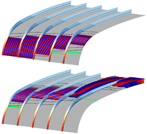
The baseflow for  $(Re_R,Re_S)=(25\,000,652)$ is presented in figures 4 and 5. This choice of set of parameters corresponds to a sweep angle $\varLambda =78.31^\circ$ for the ONERA-D airfoil, and $\varLambda =77.84^\circ$ for the Joukowski airfoil. These particularly high values compared with realistic configurations are explained by the fact that drawing neutral curves with lower sweep angles would require increasing $Re_R$, which would make the numerical computations too expensive for our current capabilities. However, the results and conclusions drawn from our theoretical study remain insightful as to the physical mechanisms involved, regardless of the value of the sweep angle. In figure 4, potential streamlines, $\delta _{99}$, and the wall-pressure coefficient $C_p=2P$ are represented in the case of ONERA-D and Joukowski airfoils. In this figure, the two represented airfoils have the same spanwise extension, but the radial and chordwise extensions of the domains are different, as described in the § 2.3.

Figure 4. Baseflow for  $(Re_R=25\,000,Re_S=652)$, which corresponds to $(Re_Q=3.38 \times 10^7,\varLambda =78.31^\circ )$ for the ONERA-D airfoil (a) and $(Re_Q=3.49 \times 10^7,\varLambda =77.84^\circ )$ for the Joukowski airfoil (b). Potential streamlines (black arrow lines) are shown. Pressure coefficient $C_p$ and boundary layer thickness $\delta _{99}$ (black line) are represented on a slice corresponding to the respective internal mesh.

Figure 5. (a) Comparison of airfoil shapes. (b–f) Baseflow for  $(Re_R=25\,000,Re_S=652)$. (b) Deflection angle $\gamma$. (c) Chordwise evolution of the ratio of $\max _\eta |U_b(s,\eta )|$ to $U_\chi ^e$ and (d) streamwise pressure gradient made non-dimensional with friction velocity $U_\tau = (\nu \partial _\eta U_{\chi }(\eta =0))^{0.5}$ and kinematic viscosity $\nu$. (e,f) Here $\varDelta$ (green), chordwise evolution of the boundary layer thicknesses, $\delta _{99}$ (red), displacement thickness $\delta ^*$ (orange), momentum thickness $\theta$ (black) and Reynolds number $Re_{\delta ^*}$ (blue) based on external streamwise velocity and displacement thickness for the (e) ONERA-D and (f) Joukowski airfoils.
In figure 5, the NACA0012 profile is used as a reference to help the reader compare and identify the properties of the two profiles studied in the paper. The three profiles are superimposed in figure 5(a). The deflection angle  $\gamma (s)=\textrm {angle}(\boldsymbol {U}^e(s),\boldsymbol {U}^\infty )$ is the angle between the direction of the external streamline ( $\boldsymbol {U}^e=(U_s^e,U_z^e)$) and the free stream velocity $\boldsymbol {U}^\infty$. It is represented in figure 5(b). Close to the attachment line, the flow is along the direction of the span $z$, so that $\gamma =90^\circ -\varLambda \approx 12^\circ$. Then, in the ONERA-D case, as $s$ increases, the $\gamma$ angle reaches a minimum of $-2.9^\circ$ at $s=0.35$ before increasing again to $-1.4^\circ$ at $s=0.15$. For the Joukowski airfoil, the $\gamma$ angle decreases on the whole domain to a value of $-2.7^\circ$ in a way similar to the case of NACA0012.
In figure 5(c) is displayed the ratio, for each  $s$-coordinate, of the CF velocity maximum $U_b(\eta )$ over the $\eta$ direction and the external streamwise velocity $U_\chi ^e$. This ratio shows that the CF component is overall weak (less than ${\approx }4\,\%$) for all airfoils and justifies an analysis in the $(\chi,\eta,b)$ orthonormal system. It also indicates where CF modes are likely to develop (high values of the ratio). In all cases, the maximum is reached around $s=0.02$. The sharp change in variation around $s=0.05$ in the case of the ONERA-D airfoil is related to the presence of two maxima of the CF velocity in the $\eta$ direction, as shown in figure 2(b). It can be noted that the presence of these two maxima leads to the presence of two inflection points, which has an impact on the destabilization of CF waves, as will be discussed in § 3.2.2. Figure 5(d) represents, as a function of $s$, the pressure gradient scaled using $U_\tau = (\nu \partial _\eta U_{\chi }(\eta =0))^{0.5}$. In the ONERA-D case, the streamwise pressure gradient is close to that of the NACA0012 airfoil and is negative up to $s=0.035$, then positive until the limit of the domain, with a flattening around $s=0.09$. This pressure-gradient changeover is typical of a flow on a swept wing and explains the existence of two inflection points in the CF velocity profile $U_b$ for some values of $s$, as shown in figure 2(b) (Arnal & Casalis Reference Arnal and Casalis2000; Wassermann & Kloker Reference Wassermann and Kloker2005). This indicates schematically that CF instabilities should be favoured for $s<0.035$ and TS instabilities after. In the case of the Joukowski airfoil, the streamwise pressure gradient remains negative up to $s=0.14$. The scaled streamwise pressure gradient reaches values of approximately $2 \times 10^{-3}$, which indicates that the gradients are only moderate. Boundary layer thickness values ( $\varDelta$, $\delta _{99}(s)$, displacement $\delta ^*(s)$, momentum $\varTheta (s)$) and Reynolds number $Re_{\delta ^*}={U_\chi ^e \delta ^*}/{\nu }$ of the ONERA-D and Joukowski airfoils are shown in figure 5(e,f). All thicknesses $\delta (s)$ are defined from the streamwise velocity profile $U_\chi (\eta )$, for example $U_\chi (\delta _{99})=0.99U_\chi ^e$. The external velocity $U_\chi ^e$ may be evaluated in the $(s,\eta,z)$ coordinate system according to $U_\chi ^e=\sqrt {(U_s^e)^2+(U_z^e)^2}$ with $U_s^e=-\int _0^{L_{\eta }} \tilde {\omega }_z \,{\rm d}\eta$ (close to $U_s^{pot}(\eta =0)$) and $U_z^e=\int _0^{L_{\eta }} \tilde {\omega }_s \,{\rm d}\eta$ (equal to $U_z^\infty$), $\tilde {\omega }_z$ and $\tilde {\omega }_s$ being the vorticity components of the baseflow along $z$ and $s$.
$s$.  $L_\eta$ is a distance to the wall sufficiently large to reach the potential region where the vorticity components are zero.
The Reynolds number  $Re_{\delta ^*}$ exhibits values between $700$ and $3900$ in the domain, which allows spatial amplification of TS instabilities for zero-pressure gradient or adverse pressure gradient boundary layers (we recall that $Re_{crit} \approx 520$ in the case of the Blasius boundary layer flow (Schmid & Henningson Reference Schmid and Henningson2001)).
3.2. Temporal chordwise-global/spanwise-local stability analysis for the ONERA-D airfoil
In order to determine the physical mechanisms involved, a classification of the types of modes studied is commonly made. The classification is based on the study of several features specific to each type of mode. As stated in the introduction, the main instabilities developing in the configurations studied here are related to AL, CF and TS types.
To help discern the type of instability, as commonly done in chordwise-local stability approaches (Arnal & Casalis Reference Arnal and Casalis2000), we introduce the  $\varPsi$ angle between the local planar wavevector $\boldsymbol {k}(s)=[{k}_s(s),k_z]$ of the mode and the direction of the external streamline: $\varPsi =\textrm {angle}(\boldsymbol {k}(s),\boldsymbol {U}^e(s))$. In the context of chordwise-global instability, we may approximate such a planar wavevector as follows: if $\hat {u}(x,y){\rm e}^{{\rm i}\beta z}$ is a component of the mode, then $(k_s,k_z)=(\partial _{s} \phi,\beta )$ where $\phi (s,\eta )=\arg {\hat {u}(s,\eta )}$. The choice of the component and wall-normal distance $\eta$ does not matter as long as the flow is weakly non-parallel (condition for the existence of such a local wavevector). Here we used the $\hat {u}_y$-component and $\eta =\delta _{99}/2$. From the literature, the following observations can be made for each of the instabilities.
(i) Attachment-line instabilities: low value of
$\varPsi$ angle, location of the direct mode and wavemaker close to the attachment line, normalized phase speed $c_z/U_z^\infty$ around $0.39$ where $c_z=\omega _r/\beta$.(ii) Cross-flow instabilities:
$\varPsi \in [80^\circ \unicode{x2013}90^\circ ]$, location of the direct mode away from the attachment line, position of the wavemaker in the region where the pressure gradient is negative and the cross-stream component of the baseflow is strong (see figure 5c,d).(iii) Tollmien–Schlichting instabilities:
$\varPsi \in [0^\circ \unicode{x2013}40^\circ ]$, location of the direct mode farther downstream, position of the wavemaker in the positive pressure gradient area.


We will try to use those criteria to distinguish the physical nature of each mode in the following. The following relation holds  $\beta =k_s(s) \tan (\varLambda +\gamma (s)+\varPsi (s))$.
3.2.1. Neutral curve in the $(Re_S,\beta \varDelta )$ plane at $Re_R=25\,000$


The search for the eigenmodes of a flow characterized by  $(Re_R,Re_S)$ is done by computing the spectrum at a given $\beta$ (examples of obtained spectra are plotted in figure 3a,c,e). By setting one of these three parameters, neutral curves can be drawn varying the two remaining ones. The neutral curve is the limit between configurations where all modes of the spectrum are stable and configurations where at least one mode is unstable. By studying the characteristics of the modes along the neutral curve, called ‘marginal modes’, one can determine the types of instability responsible for the destabilization of the flow and the physical mechanisms involved.
We have represented (solid line) in figure 6(a) the neutral curve in the  $(Re_S,\beta \varDelta )$ parameter space for $Re_R=25\,000$. Black dots indicate 10 specific marginal eigenvalue/eigenvectors, labelled (i) (largest spanwise wavenumber) to (x) (smallest wavenumber). These modes are listed in table 3. Their spatial structure will be analysed in detail in the next section, and more specifically the modes (i), (vi) and (ix) noted with an asterisk in table 3 and in red in figure 6. The presence of kinks along the neutral curve indicates that marginal modes with different features may be responsible for instability, depending on the spanwise wavenumber. A detailed study (not shown here) of regions in the vicinity of the kinks confirms the presence of several unstable modes. The neutral curve is composed of the overlapping of six distinct curves (which will be called ‘lobes’) in the present case, each represented by a different colour in figure 6. The prolongation of each partial neutral curve in the ‘unstable’ region is indicated by dashed lines.

Figure 6. (a) Neutral curve (solid line) of ONERA-D airfoil in  $(Re_S,\beta \varDelta )$ plane at $Re_R=25\,000$ and SHF neutral curve (orange dotted line) from Obrist & Schmid (Reference Obrist and Schmid2003). The six different ‘lobes’ composing the full neutral curve are displayed in different colours. (b) Phase speed in the spanwise direction of marginal modes of ONERA-D airfoil at $Re_R=25\,000$. The coloured lines indicate the lobes to which the modes belong to. In (a,b), dashed lines refer to the prolongation of the solid line in the ‘unstable’ domain. Modes from table 3 are indicated with black dots, modes (i), (vi) and (ix) being circled in red.
Table 3. The  $(Re_S,\beta \varDelta )$ value of 10 marginal modes, listed in decreasing order of $\beta$, for $Re_R=25\,000$. The phase speed in the spanwise direction $c_z/U_z^\infty$ is also shown. Asterisk-noted modes will be analysed in detail in the next part.

The critical sweep Reynolds number is  $Re_{S,crit}=527$ and is reached for $\beta _{crit} \varDelta =0.057$.
We notice that the upper lobe (in dark blue) fits relatively well with the upper part of the neutral curve of the SHF (Obrist & Schmid Reference Obrist and Schmid2003), shown with an orange dotted line. As we will see in the § 3.2.3, the modes associated with this lobe are of AL type. They are thus located close to the attachment line and are almost invariant in the CF  $b$ direction. At the attachment line, we have $(\chi,\eta,b)=(z,-x,y)$ and $s=y$. This lobe also corresponds to large values of $\beta$. The high value of $\beta$ implies a large variation in the $z$ direction, but also in the $x$ direction due to the continuity equation and the invariance in $y$ direction. The small structures of the modes in the $(x=\eta,z)$ plane imply that they will be less impacted by the variation of the curvature in the $s$ direction. Therefore, the less dependent they are on the radius of curvature $r_c$ of the leading edge. The limit corresponds to the SHF configuration for which $r_c=\infty$. For the other lobes at lower values of $\beta$, the leading-edge radius of curvature $r_c$ and therefore $Re_R$ must have a greater influence. Yet, the curvature explains why the critical value of the Reynolds number of the upper lobe (dark blue), $Re_{S,crit} \approx 621$, is different from the one given in Obrist & Schmid (Reference Obrist and Schmid2003) and Lin & Malik (Reference Lin and Malik1996) for the SHF, which is $Re_{S,crit}\approx 582$. This is confirmed by Lin & Malik (Reference Lin and Malik1997) who studied the effect of $Re_R$ on attachment line instabilities and determined the values $Re_{S,crit}= 637.6$ and $Re_{S,crit}= 599.5$ for $Re_R=10\,000$ and $Re_R=100\,000$, respectively. An interpolation for $Re_R=25\,000$ yield a value $Re_{S,crit}\approx 620$, which is close to the value we find.
The associated phase speed  $c_z =\omega _r / \beta$ normalized by the spanwise baseflow velocity $U_z^\infty$ is represented in figure 6(b) as a function of the spanwise wavenumber $\beta \varDelta$. The lobe changes result in discontinuities of the phase speed, which confirm that the marginal modes of the different lobes have distinct features. The same colour code as in figure 6(a) has been used to ease the correspondence of the lobes. The upper lobe (dark blue) is characteristic of AL instabilities with phase speeds close to those of TS waves in Blasius boundary layer $c_\chi /U_\chi ^\infty \approx 0.39$ where $c_\chi =\omega _r/k_\chi$ (see Schmid & Henningson (Reference Schmid and Henningson2001)). In the close vicinity of the attachment line, the values obtained in the case of the Blasius boundary layer are comparable to those of $c_z/U_z^\infty$ insofar as $\chi$ and $z$ directions are equal and the streamwise pressure gradient is zero (see figure 5d). As the spanwise wavenumber decreases, the phase speed of the marginal modes decreases until values around $c_z/U_z^\infty \approx 0.27$ reached for $\beta \varDelta \approx 0.1$. The phase speed on the two lowest lobes (red and purple) is in strong contrast with the phase speed of the previous ones since it jumps up to $c_z/U_z^\infty \approx 0.32$ at $\beta \varDelta \approx 0.1$. We also note that except for the upper (dark blue) and lower (purple) lobes, the phase speed of the lobes decreases almost linearly with the decrease of $\beta$. The change in variation for the lower lobe, around $\beta \varDelta =0.07$ may indicate a change in the nature of the modes.
3.2.2. Study of modes (i), (vi) and (ix) at $Re_R=25\,000$

We now analyse the spatial structure of marginal modes, and in particular modes (i), (vi) and (ix) in table 3. Figure 7(a) shows, for each of these three marginal modes, two isosurfaces of the real part of the vertical velocity perturbation  ${\rm Re}(\hat {u}_y(x,y){\rm e}^{{\rm i}\beta z})$ at $\pm 0.01$ times the absolute maximum (red and blue), the wavemaker region (green), the pressure coefficient $C_p$ of the baseflow (shown on the vertical planes) and the boundary layer thickness $\delta _{99}$ (black solid line on the vertical planes). An example of $\varPsi$ angle is drawn for mode (vi), with $\boldsymbol {k}$ designating the local planar wave vector of the mode. For mode (i), the wavemaker is not seen because it is covered by the isosurfaces of the direct mode. With this display, the perturbations seem also strong outside the boundary layer ( $\eta >\delta _{99}$). In fact, the extremal values are found at positions around $\delta _{99}/2$ in the $\eta$ direction, as shown in figures 7(b)–7(d) where $\delta _{99}$ and the real part of the vertical velocity perturbation in the $(s,\eta )$ plane are drawn. In figures 7(e)–7(g) are plotted the normalized magnitude as a function of $s$ of the wavemaker (green line), direct mode (blue line) and adjoint mode (red line). The $\varPsi$ angle at altitude $\eta =\delta _{99}/2$ of the vertical velocity component of the perturbation is represented in figures 7(h)–7(j). The oscillations observed in figure 7(h,j) occur when the mode magnitude is low or the orientation changes abruptly. We have checked that they are not due to insufficient refinement of the mesh since automatic adaptations based on the modes and their wavemaker have been tried, without removing these oscillations.

Figure 7. Spatial structure of the real part of the vertical velocity perturbation  ${\rm Re}(\hat {u}_y(x,y){\rm e}^{{\rm i}\beta z})$ of modes: (i), (b,e,h); (vi), (c,f,i); and (ix), (d,g,j). (a). For each mode two isosurfaces at $\pm 0.01$ times the absolute maximum are represented in red and blue. The baseflow pressure field $C_p$ (red and blue isocontours with the same colourbar as in figure 4a) and boundary layer thickness $\delta _{99}$ (black line) are shown in the vertical planes separating the modes. The wavemaker region is sketched by a green isosurface at $95\,\%$ of its maximum value. Several external streamlines of the baseflow are shown (black arrow lines). An example of wavevector and $\varPsi$ angle is also displayed for mode (vi). (b–d) The plot in the $(s,\eta )$ plane as a proportion of the absolute maximum. Here $\delta _{99}$ is displayed (black line). (e–g) The normalized magnitude of direct mode (blue), adjoint mode (red) and wavemaker (green). Position of the zero pressure gradient (red dashed line) and of the maximum of the ratio $\max _\eta |U_b(s,\eta )|$ to $U_\chi ^e$ (black dashed line) are indicated. (h–j) The chordwise evolution of the $\varPsi$ angle.
Concerning mode (i), we notice in figure 7(a,e) that the direct mode and the wavemaker are located close to the attachment line, the magnitude being vanishingly small for  $s>0.03$. Moreover, figure 7(a,h) reveals that the $\varPsi$ angle is low $(0^\circ \unicode{x2013}15^\circ )$ in the vicinity of the attachment line zone, where the mode is strongest. In the low-magnitude region, it is seen that the $\varPsi$ angle is greater than $80^\circ$. These features are common to all the upper lobe modes (dark blue lobe) that have been calculated. Unlike reported in Meneghello et al. (Reference Meneghello, Schmid and Huerre2015) for a stable mode of the flow around a Joukowski airfoil, we do not find a second high magnitude region where the modes have CF characteristics.
Even if the change of  $\varPsi$ angle at $s\approx 0.05$ is reminiscent of the ‘connected modes’ described by Mack et al. (Reference Mack, Schmid and Sesterhenn2008) in the case of a compressible supersonic swept flow around a parabolic body, the low amplitude and high damping of the mode where it exhibits CF characteristics is such that we will not define it as a connected mode.
For mode (vi), we can see in figure 7(a,f) that the mode is located farther downstream but that the wavemaker remains localized in the negative pressure gradient zone. The magnitude of the direct mode increases in the negative pressure gradient zone ( $s<0.035$) and starts to decrease in the positive pressure gradient zone ( $s>0.035$). In figure 7(a,i), we find that the $\varPsi$ angle increases with $s$ from $30^\circ$ to $60^\circ$ in the area where the wavemaker is maximum. The $\varPsi$ angle at the maximum magnitude of the direct mode is greater than $80^\circ$. From these observations, we can conclude that this mode is of the CF type.
In figure 7(a,g), we observe that the direct mode and the wavemaker are located farther along the chord, where the pressure gradient is positive. Moreover, the direct mode extends over a significantly greater range and admits two local maxima (at  $s=0.06$ and $s=0.127$). In figure 7(a,j), we find a $\varPsi$ angle of $60^\circ$ at the location where the magnitude of the wavemaker is maximum and the direct mode reaches its first local maximum of magnitude. However, at the location of the global maximum of the direct mode, the $\varPsi$ angle is equal to $23^\circ$.
Thus, we have the presence of two distinct spatial amplifications where the spatial structure of the direct mode exhibits features corresponding to distinct types of instability at the two amplitude maxima: CF for the first and TS for the second. We can then define this as a CF/TS connected mode, the existence of which, to the authors’ knowledge, had not yet been documented.
To better characterize this mode and understand the interplay between both mechanisms, figure 8(a) represents the evolution with  $s$ of ${\partial U_b}/{\partial \eta }$ at the level of the inflection points of the velocity profile $U_b$. We observe that for $s>0.35$, i.e. near the change of sign of the pressure gradient (represented in figure 5d), a second inflection point appears. The solid line corresponds to the inflection point farthest from the wall, while the dashed line corresponds to the one close to it. This quantity is related to the strength of the CF instability mechanism, and we notice that the inflection point closest to the wall is the most critical one when it exists. These two inflection points are represented on the profile of $U_b$ plotted in figure 8(b) for the coordinate $s=0.053$, which corresponds to the position where the wavemaker of the mode (ix) is maximal. The wavemaker profile at the position $s=0.053$ is also shown in figure 8(c). At this position, the wavemaker reaches its maximum for $\eta =2.6\times 10^{-4}$, which coincides with the position of the most critical inflection point.

Figure 8. (a) Evolution according to  $s$ of ${\partial U_b}/{\partial \eta }$ at the inflection points of the CF velocity wall-normal profile. The inflection point farthest from the wall corresponds to the black solid line and the second (when it exists) to the black dashed line. The positions of the pressure-gradient changeover (blue dotted line at $s=0.035$) and of the maximum of the wavemaker magnitude of the mode (ix) (green dotted line at $s=0.053$) are shown. Wall-normal profiles of the CF velocity (b) and the wavemaker (c) at $s=0.053$ are plotted. The inflection points farthest and closest from the wall are represented by solid and empty dashed black circles, respectively. The maximum of the wavemaker in the wall- normal direction coincides with the inflection point closest to the wall, which is the most critical.
Therefore, although the dominant spatial structure is that corresponding to the TS type, the location of the wavemaker at an inflection point of the CF velocity with high values of  ${\partial U_b}/{\partial \eta }$ suggests that the physical mechanism responsible for the initial spatial amplification and overall destabilization of the mode is related to the CF instability. Moreover, the position of the wavemaker in a zone where the pressure gradient is positive justifies that the TS-like spatial structure develops. The presence of such CF/TS connected modes is related to the pressure-gradient changeover typical of a swept wing. Indeed, this configuration allows for CF velocity profiles with strong enough shear to trigger CF instabilities, located in strongly positive pressure gradient regions that allow TS type spatial amplification. This type of flow had not been studied in previous chordwise-global stability analyses (Mack et al. Reference Mack, Schmid and Sesterhenn2008; Meneghello et al. Reference Meneghello, Schmid and Huerre2015). The stability of a profile with a pressure-gradient changeover had only been studied in a chordwise-local context by Wassermann & Kloker (Reference Wassermann and Kloker2005) and although CF and TS modes were observed, no mode with both features was found. This can be partly explained by the fact that modes with such abrupt spatial structure changes are particularly difficult to identify in a chordwise-local framework.
3.2.3. Modes between modes (i), (vi) and (ix) at $Re_R=25\,000$

We have seen through the analysis of modes (i), (vi) and (ix), that there is a great diversity of marginal modes in our configuration. In order to better understand how the different instabilities are related along the neutral curve, the whole set of marginal modes is studied in this part. Figure 9 shows all the modes referenced in table 3, similarly to figure 7(a).

In figure 10 the magnitude of the direct and adjoint marginal modes are plotted, as well as their wavemaker and the  $\varPsi$ angle as a function of $s$ with $\beta \varDelta$ ranging from $0.034$ to $0.33$, in increments of $0.01$. The delimitations between the different lobes introduced in figure 6 are indicated with black horizontal lines, and the wavenumber $\beta \varDelta$ of the different modes of table 3 are indicated by green ticks on the right. The chordwise coordinate of the maximum magnitude of the direct mode (red circles) and adjoint modes (yellow circles), as well as the position where the pressure gradient is zero (red vertical dotted line) are indicated. In figure 10(d), only the $\varPsi$ angles for locations where the magnitude of the direct mode is greater than $10^{-2}$ have been shown.

Figure 10. Normalized magnitude of direct mode (a), adjoint mode (b) and wavemaker (c) and  $\varPsi$ angle (in degrees) (d), as a function of $s$ for marginal modes with $\beta \varDelta$ ranging from $0.034$ to $0.33$ in increments of $0.01$. The $\beta \varDelta$ ordinate of the delimitation between lobes (black horizontal lines), chordwise position of zero pressure gradient (red dotted line) and chordwise position of maximum magnitude of wavemakers (green circles) and direct (red circles) and adjoint (yellow circles) modes are indicated.
The first comment in figures 9 and 10 is that, in addition to the modes described in § 3.2.2, we observe modes with more diverse features. Moreover, we notice in figure 10 that these characteristics are closely related to the belonging to particular lobes. For all lobes, except between the last two, abrupt changes in the magnitude and/or  $\varPsi$ angle are noted. This observation confirms once again the presence of distinct instabilities between lobes. The last two lobes have been distinguished only from discontinuities in the phase speed curve in figure 6(b).
Concerning the upper lobe (dark blue), we see, with figure 10 and modes (i) and (ii) of figure 9, that its marginal modes fall into the characteristics of AL modes with a direct mode and a wavemaker located close to the attachment line and isophases perpendicular to the streamwise direction (low  $\varPsi$ angle).
For the grey and green lobes of figure 6, figure 10 and modes (iii) and (iv) of figure 9 show that their marginal modes are still close to the attachment line but with a location (as well as the wavemaker one) slightly shifted in the chordwise direction and the  $\varPsi$ angle at the maximum magnitude of the direct mode starting to increase: the modes start transitioning to CF-like modes.
In the case of the light blue lobe, as illustrated by modes (v) and (vi), marginal modes are located even farther downstream and their maxima are now close to the region of minimal  $C_p$. Mode (v) exhibits a highly localized distribution in the chordwise direction, with a strong increase of the perturbation magnitude in the accelerated region before a sharp decrease in the decelerated one. Yet, contrary to before, the wavemaker region is now located fully in the accelerated region and in the area where the ratio of the CF velocity to the streamwise velocity is highest, as shown in figure 5(c). The isophases of the perturbations are nearly aligned with the streamlines of the external flow ( $\varPsi$ angle close to $90^\circ$). These modes are fully of CF type. Contrary to the stable mode described in Meneghello et al. (Reference Meneghello, Schmid and Huerre2015), the CF marginal modes observed here have wavemakers that are not localized at the attachment line, thus indicating that efficient control of these instabilities in the considered case cannot be restricted to the attachment line area.
Figure 10(a,c) show that direct modes and wavemakers of the last two lobes are fully localized in the decelerated region. As shown in figure 9, for modes (vii) and (viii), the chordwise magnitude distribution exhibits a strong amplification before the maximum magnitude and weak damping afterward. The  $\varPsi$ angle is very close to $90^\circ$. These are modes which have CF characteristics even if the wavemaker is in the decelerated region.
For the last two modes (ix) and (x), we notice a sharp change, both in the orientation of the modes and their location. Indeed, the  $\varPsi$ angle is close to $10^\circ$ (as for modes (i) and (ii)) and their location is even more downstream and more extended in the chordwise direction than before. On the other hand, the wavemaker region has nearly not moved and is still at the beginning of the decelerated region. As revealed in figure 10, along the lower lobe, we switch from a situation with a single magnitude maximum for the direct mode and a $\varPsi$ angle relatively high (CF type mode) to a direct mode with two local magnitude maxima, the first still of CF type (large angle) but the second (the global one) being much farther away and corresponding to a location where the $\varPsi$ angle is low (reminiscent of TS type). For $\beta <0.05$, although the direct modes could continue to grow downstream, the maximum magnitude is located at $s=0.165$, which corresponds to the end of the domain. Contrary to the direct mode, we observe that the magnitude of the adjoint mode evolves very weakly as a function of $\beta \varDelta$ and reaches the location of positive pressure gradient around $\beta \varDelta \approx 0.073$, which is the $\beta \varDelta$ value where the magnitude and orientation of direct modes vary abruptly. This value of $\beta \varDelta \approx 0.073$ also corresponds to the value at which the phase speed curve of the lower lobe in figure 6(b) starts to decrease again.
In the case of very stable modes, we observe even more varied features. In Appendix C the spatial structure of the mode studied by Meneghello in the case of a Joukowski airfoil is represented (Meneghello et al. Reference Meneghello, Schmid and Huerre2015) and, by considering the orientation of the direct mode, we note a mode mainly of CF type but with a double amplification and a wavemaker contained in the attachment line.
3.3. Absolute/convective stability analysis in the spanwise $z$ direction

We will now follow the methodology described in the § 2.2.4 to study the convective or absolute nature in the spanwise direction of some instabilities.
In the case  $(Re_R,Re_S)=(25\,000,652)$, figure 11 shows the imaginary part of the most unstable eigenvalue with respect to $\beta \varDelta$. We notice the presence of several parabolas similar to those noted in Mack et al. (Reference Mack, Schmid and Sesterhenn2008), Mack & Schmid (Reference Mack and Schmid2011) and which are related to the crossing of the different lobes. A maximum of $\omega _i$ is reached for three values of $\beta ^{peak}\varDelta$: $0.285$, $0.187$ and $0.062$, with respective spanwise group velocities $V_g^{peak}={\partial \omega _r}/{\partial \beta }|_{\beta =\beta ^{peak}}$: $2.147$, $2.065$ and $1.736$. The marginally stable modes (i), (vi) and (x) introduced in the table 3 are indicated with black dots circled in red.

Figure 11. Imaginary part of the most unstable eigenvalue at  $(Re_R,Re_S)=(25\,000,652)$ for $\beta \varDelta$ ranging from $0.03$ to $0.35$ in increments of $0.1$. Points where $\omega _i$ reaches a maximum is depicted (red dots) and corresponding spanwise group velocity is shown. The marginal modes (i), (vi) and (x) referenced in the table 3 are marked with black dots circled in red.
In figure 12 are represented the evolutions of  $(\omega _{V_g},\beta _{V_g}\varDelta )$ with the decrease of $V_g$ values from the three initial couples $(\beta ^{peak}\varDelta,V_g^{peak})$: $(\beta _{init,1}\varDelta,V_{g,init,1})=(0.28,2.147)$, $(\beta _{init,2}\varDelta,V_{g,init,2})=(0.19,2.065)$ and $(\beta _{init,3}\varDelta,V_{g,init,3})=(0.06,1.736)$. For each case, we made steps in $V_g$ of size $V_{g,init}/300$. The variation of $\omega _{V_g,i}$ as a function of $V_g$ is specifically shown in figure 13 for the three initial configurations considered. Note that the ‘steps’ that can be observed for $(\beta _{init,1}\varDelta,V_{g,init,1})$ have no physical meaning and are rather related to the definition of the stopping criteria. The spanwise group velocities are only decreased down to $1.934$, $1.837$ and $1.644$ for $(\beta _{init,1}\varDelta,V_{g,init,1})$, $(\beta _{init,2}\varDelta,V_{g,init,2})$ and $(\beta _{init,3}\varDelta,V_{g,init,3})$, respectively. As the modes to be computed move away in chord with the decrease of $V_g$, the chord extension of the mesh used was not sufficient when the value of $V_g$ was too low. However, the $\omega _{V_g,i}$ values being negative and $\omega _{V_g,i}$ decreasing with the $V_g$ values (Huerre Reference Huerre2000), we assume that no unstable modes would have been found at $V_g=0$ in the studied flow conditions. Furthermore, we can note that according to the starting couple $(\beta _{init}\varDelta,V_{g,init})$, $\omega _{V_g}$ decreases more or less slowly with the value of $V_g$. Thus, as in the present case, the initial couple to investigate to find the unstable mode at $V_g=0$ is not necessarily the most unstable one for $\beta \in \mathbb {R}$.

Figure 12. (a) Here  $\omega _{V_g}$ and (b) $\beta _{V_g}\varDelta$ at several $V_g$ for the three $(\beta \varDelta,V_g)$ inital values: $(0.28,2.147)$ (in blue); $(0.19,2.065)$ (in indigo); and $(0.06,1.736)$ (in black). The initial values are represented in green and the spanwise group velocity $V_g$ of some $(\omega _{V_g},\beta _{V_g}\varDelta )$ displayed in red are indicated.

Figure 13. Here  $\omega _{V_g,i}$ as a function of $V_g$ for the three $(\beta \varDelta,V_g)$ initial values: $(0.28,2.147)$ (in blue); $(0.19,2.065)$ (in indigo); and $(0.06,1.736)$ (in black).
The flow at  $(Re_R,Re_S)=(25\,000,652)$ is, a priori, only convectively unstable in the spanwise direction. An identical study for $(Re_R,Re_S)=(25\,000,800)$ gave an equal conclusion. To be more conclusive about the convective or absolute nature of the boundary layer instabilities of the flow around ONERA-D, it would be necessary to evaluate a large number of values of $(Re_R,Re_S)$. However, these first results and those reported by previous studies in the literature (Lingwood Reference Lingwood1997; Taylor & Peake Reference Taylor and Peake1998, Reference Taylor and Peake1999; Türkylmazoglu & Gajjar Reference Türkylmazoglu and Gajjar1999), indicate that no absolute instability in $(x,y,z)$ is expected to be found.
3.4. Effect of $Re_R$ for the ONERA-D airfoil

In figure 14 are superimposed the neutral curves corresponding to different values of  $Re_R$, as well as the neutral curve of the SHF from Obrist & Schmid (Reference Obrist and Schmid2003). The number of lobes of the neutral curves tends to increase as $Re_R$ increases: for $Re_R=10\,000$, only two lobes are observed, while for $Re_R=25\,000$, six can be seen, and around 10 for $Re_R=50\,000$.

Figure 14. Comparison of neutral curves of ONERA-D at various  $Re_R$ values and SHF neutral curve from Obrist & Schmid (Reference Obrist and Schmid2003). The SHF neutral curve is plotted in dashed orange line and ONERA-D neutral curves for $Re_R=10\,000$, $Re_R=25\,000$ and $Re_R=50\,000$ are drawn, respectively, in blue, green and black.
We can see that the upper lobe, linked to AL instabilities, fits better with the neutral curve of the SHF as  $Re_R$ increases. As described by Lin & Malik (Reference Lin and Malik1997), the increase in $Re_R$ leads to a slight increase in $\beta$ of the upper part of the lobe and to a slight decrease of its critical Reynolds number, $Re_{S,crit,AL}$ going from $609$ to $601$ for $Re_R=25\,000$ and $Re_R=50\,000$, respectively. Overall, the upper lobe is only weakly impacted by the value of $Re_R$.
On the other hand, all the other lobes are strongly stabilized with the increase of  $Re_R$ and shifted to larger $Re_S$ values. For values of $Re_R$ lower than $Re_R\approx 30\,000$, the most critical marginal mode belongs to the lower lobe, bringing the critical value of $Re_S$ to values lower than $595$. For $Re_R=25\,000$ and $Re_R=10\,000$, we have values of $Re_{S,crit}$ at $521$ and $429$, respectively. For values of $Re_R>50\,000$, we can presume that non-AL instabilities are stabilized enough to find thresholds close to the ones predicted by Lin & Malik (Reference Lin and Malik1996), i.e. around $Re_S=600$. For $Re_R=50\,000$, we find $Re_{S,crit}=601$, which is close to $Re_S\approx 610$ that we can expect for SHF at $Re_R=50\,000$ by interpolating the values given by Lin & Malik (Reference Lin and Malik1997) for $Re_R=10^4$ and $10^5$.
The parametric study based on the value of the parameter  $Re_R$ was not pursued for larger values because this would lead to numerical difficulties, including the need to use a significantly finer mesh. Moreover, as previously mentioned, the consideration of a high $Re_R$ makes the structure of the neutral curve more complex, with an increase in the number of lobes, and its detailed study would be difficult. However, it can be noted that for $Re_R=100\,000$, a study at $Re_S=620$ confirmed that the unstable modes are only of AL type with high values of $\beta \varDelta$.
In conclusion, from these observations and from the study of the instabilities associated with the different lobes, we can deduce that the parameter  $Re_R$ has a more or less significant influence according to the nature of the instabilities involved, the AL ones being the least stabilized with the increase of $Re_R$.
3.5. Comparison of neutral curve with a Joukowski airfoil as a function of $Re_S$ at $Re_R=25\,000$ and as a function of $Re_Q$ at $\varLambda =80.03^\circ$


In order to study the influence of the airfoil, we compare the neutral curves of the ONERA-D airfoil and the Joukowski airfoil of thickness parameter  $\epsilon =0.1$. Neutral curves at $Re_R=25\,000$ are drawn in figure 15(a). A comparison of some characteristic of both baseflow at $Re_S=652$ is shown in figure 5. In both cases, we observe a neutral curve composed of several lobes. For the Joukowski airfoil, the lower lobe reaches its critical value at a smaller $\beta$. The critical Reynolds number is reached at $\beta \varDelta \approx 0.20$ and $Re_{S,c,Jouk}=517$, thus the Joukowski airfoil is less stable than the ONERA-D in these conditions. The study of some marginal modes (not shown here), in particular on the lower lobe shows important differences in the spatial structure between the Joukowski and ONERA-D cases. Indeed, due to the negative pressure gradient extending farther in the chord in the Joukowski case, the observed marginal modes are located farther downstream and do not show TS features.

Figure 15. Comparison between neutral curves of ONERA-D (blue line) and Joukowski airfoils (red line): (a) as a function of  $Re_S$ at $Re_R=25\,000$; (b) a function of $Re_Q$ at $\varLambda =80.03 ^\circ$. The latter case describes the stability characteristics of a wing at sweep $80.03^\circ$ when, for example, the inflow velocity is increased.
In order to assess the differences between the two airfoils with an applied point of view, we now compare the neutral curves using the flow parameters  $(Re_Q,\varLambda )$ introduced in § 2.1, since the two simplest parameters that can be varied independently in a wind tunnel are the upstream infinite velocity $U^\infty$ and the sweep angle $\varLambda$. In figure 15(b) are superimposed the neutral curves of the ONERA-D and Joukowski airfoils in the $(Re_Q, \beta \varDelta )$ plane by setting $\varLambda =80.03^\circ$; this implies a joint variation of $Re_R$ and $Re_S$. The critical Reynolds numbers are $Re_{Q,c,ONERA-D}=1.34 \times 10^7$ (corresponding to $(Re_{R,c},Re_{S,c})=(7229,413)$) and $Re_{Q,c,Jouk}=1.12 \times 10^7$ (corresponding to $(Re_{R,c},Re_{S,c})=(5414,372)$) and the neutral curve of ONERA-D is included in the Joukowski curve. We can conclude that for $\varLambda =80.03^\circ$, the ONERA-D airfoil is more stable than the Joukowski airfoil. This conclusion was expected for instabilities with TS features since ONERA-D was designed to stabilize them, but it was more difficult to make an early opinion on CF instabilities. The lesser stability of the Joukowski airfoil compared with the ONERA-D at low $\beta$ may be related to the fact that it also corresponds to low $k_\chi$ and modes with $k_\chi =0$ correspond to TS instabilities.
Such a neutral curve was drawn according to  $(\beta,Re_S)$ by Mack & Schmid (Reference Mack and Schmid2011) for a compressible flow around a parabolic body with a radius of curvature of $0.1$ at a swept angle of $\varLambda =72.38 ^\circ$. The authors observed the presence of a single lobe with a critical value $Re_{S,c}\approx 375$. This difference can be explained by the fact that the neutral curve was computed in a supersonic regime with $Ma_S={W_\infty }/{c_\infty }=1.25$ where $c_\infty$ corresponds to the speed of sound, and by the difference in the value of the radius of curvature of the studied airfoils.
4. Conclusion
In this paper, we investigated the boundary-layer instabilities of an incompressible flow around a swept ONERA-D and Joukowski airfoils with infinite span and no incidence. Temporal chordwise-global stability analyses have been performed on a domain covering the whole leading-edge. We first focused on the case of the ONERA-D airfoil at  $Re_R=25\,000$ by computing the neutral curve according to the sweep Reynolds number $Re_S$ and the spanwise wavenumber $\beta$. The composite nature of the neutral curve has been evidenced and several overlapping regions, or ‘lobes’, have been identified. A justification for the existence of different lobes constituting the total neutral curve could be made on a physical basis by considering the kinks of the neutral curve, the presence of multiple unstable modes at the overlap of the lobes as well as the changes in phase speed and spatial structure of the marginal modes between the different lobes. A detailed study of the marginal modes was conducted based on the spatial structure of the direct and adjoint modes in addition to the position of the wavemaker, in connection with the streamwise pressure gradient and the three-dimensionality of the baseflow. This study revealed the presence of marginal modes of AL and CF type, as well as modes that do not fall into standard classifications of one particular type. We identified modes with two distinct spatial amplifications, the first amplification being related to a CF-like spatial structure of the direct mode while the second amplification is associated with a spatial structure reminiscent of TS instabilities. These modes have been defined as connected CF/TS mode where the dominant spatial structure is close to TS waves but the physical mechanism responsible for the instability is related to a CF mechanism. To the authors’ knowledge, a mode with a connection of this nature has not been previously reported. However, no clear connected AL/CF modes have been identified.
The absolutely or convectively unstable nature of the flow in the spanwise direction was also tackled, by using chordwise-global stability analyses. Our results suggest that the flow is only convectively unstable in the spanwise direction. To the authors’ knowledge, this is the first study to address this issue in a chordwise-global framework.
We then did a parametric study by comparing neutral curves of ONERA-D at three values of  $Re_R$. It reveals that the increase of $Re_R$ has a greater stabilizing effect on CF and TS modes than AL ones. The increase of $Re_R$ also implies an increasing number of lobes, as well as a neutral curve that tends to be closer to that of the SHF. Therefore, for $Re_R>30\,000$, the AL instabilities lobe becomes the most critical ones.
A measure of the influence of the airfoil geometry was made by comparing two neutral curves of the Joukowski (with parameter thickness  $\epsilon =0.1$) and ONERA-D airfoils at given $Re_R$ and sweep $\varLambda$. For $Re_R=25\,000$, for both airfoils, several lobes are noticed and the critical sweep Reynolds number is close but the critical spanwise wavenumber is significantly higher for the Joukowski case than for the ONERA-D case. The comparison at $\varLambda =80.03^\circ$ reveals that, under the conditions studied, the ONERA-D airfoil is more stable than the Joukowski airfoil for every spanwise wavenumber.
Acknowledgements
The help of L. Pascal and J.-P. Brazier in setting up the boundary layer code calculations and the chordwise-local stability analyses is gratefully acknowledged.
Funding
The study was supported by a grant from the Agence de l'innovation de défense (Defence Innovation Agency). This project has received funding from the European Research Council (ERC) under the European Union's Horizon 2020 research and innovation program (grant agreement no. 638307).
Declaration of interests
The authors report no conflict of interest.
Appendix A. Adjoint operators
The adjoint eigenvalue–eigenvector problem is the following:
 \begin{equation} \mathcal{L}^{\dagger}\boldsymbol{\hat{q}^{\dagger}}=\omega^{\dagger}\mathcal{B}^{\dagger}\boldsymbol{\hat{q}^{\dagger}}. \end{equation}
 By using the definition of the adjoint operator presented in (2.15) and integration by parts, we get  $\mathcal {B}^{\dagger} =-\mathcal {B}$ and the adjoint operator $\mathcal {L}^{\dagger}$:
 \begin{equation} \mathcal{L}^{\dagger}{=} \left[ \begin{array}{@{}cccc@{}} \partial_x U-\mathcal{C}_\beta-\mathcal{D}_\beta & \partial_x V & \partial_x W & -\partial_x \\ \partial_y U & \partial_y V-\mathcal{C}_\beta-\mathcal{D}_\beta & \partial_y W & -\partial_y \\ 0 & 0 & -\mathcal{C}_\beta-\mathcal{D}_\beta & -i\beta \\ -\partial_x & -\partial_y & -{\rm i}\beta & 0 \end{array} \right]. \end{equation}
Appendix B. Comparison with chordwise-local stability analyses
In our study, we used chordwise-global perturbations of the form  $\boldsymbol {q}=\hat {\boldsymbol {q}}(x,y) \exp ({{\rm i}(\beta z -\omega t)})$. Most of the stability analyses done to date have been done using chordwise-local analyses with chordwise-local eigenmodes sought in the $(s,\eta,z)$ reference frame in the form $q=\hat {q}(\eta )\exp ({{\rm i}(\alpha s + \beta z - \omega t)})$. Their spatial amplification rate is defined as $\ln ({{A}/{A_0}})=\int _{s_0}^s-{\rm Im}(\alpha )\,{\rm d}s$ (see for instance Arnal & Casalis (Reference Arnal and Casalis2000) or Reed, Saric & Arnal (Reference Reed, Saric and Arnal1996) for reviews on chordwise-local stability approach). We can mention that the presence of chordwise-globally unstable modes implies a chordwise-local absolute unstable flow (Huerre & Monkewitz Reference Huerre and Monkewitz1990). In order to validate the results obtained with our chordwise-global method, we compare the spatial structures obtained with a chordwise-local stability analysis for $\beta$ and $\omega$ provided by the chordwise-global stability analysis. We conducted such an analysis for the marginal modes (vi) and (viii), so that both $\omega$ and $\beta$ are real. The spatial stability analysis in the $s$ direction is solved for these fixed $\beta$ and $\omega$ real values. The chordwise-local stability code solves the one-dimensional differential eigenvalue problem with a high-order scheme. The parallel flow assumption is used, and the flow computed by the boundary-layer solver is used as the baseflow, to avoid interpolation errors from the finite element method mesh. In the chordwise-local stability analysis framework, the $\varPsi$ angle is directly derived from the real parts of $\alpha$ and $\beta$ and the knowledge of the inviscid streamwise direction at each chordwise location. The comparison between chordwise-global and chordwise-local stability results is displayed in figure 16.

Figure 16. Comparison of magnitude (a,b) and  $\varPsi$ (c,d) between chordwise-local (in red) and chordwise-global (in blue) analyses for modes (vi) (a,c) and (viii) (b,d).
An agreement of the  $\varPsi$ vectors is observed for chordwise-local and chordwise-global analyses in both cases. The magnitude is also close with magnitude maxima at almost identical positions. Thus, we obtain close results, which validate the use of the chordwise-global stability analysis. The latter method has the advantage of being able to identify the whole structure of the modes at once, without parallel flow assumptions, and to directly identify the absolute/convective nature in the chordwise direction.
Appendix C. Stability results at $(Re_R,Re_S,\beta \varDelta )=(16\,129,113,0.45)$ for a Joukowski airfoil

We report here the results we obtain in a case similar to Meneghello et al. (Reference Meneghello, Schmid and Huerre2015), i.e. under the conditions  $(Re_R,Re_S,\beta \varDelta )=(16\,129,113,0.45)$ with a Joukowski airfoil of thickness parameter $\epsilon =0.1$, with no incidence and of infinite span. These conditions correspond to a highly stable case.
In table 4,  $\omega /(\beta U^\infty _z)$ of the three least stable symmetric eigenvalues are presented. We observe a relative error lower than $0.5\,\%$ for the three eigenvalues.
Table 4. The  $\omega /(\beta U^\infty _z)$ of the three least stable symmetric eigenvalues.

In figure 17(a) is drawn the magnitude of the direct and adjoint modes, as well as the wavemaker, as a function of  $s$. We note a first growth of the magnitude of the direct mode until $s=0.02$, then a decrease until $s=0.05$, followed by a second growth from $s=0.05$ until the end of the domain. The wavemaker is located at the attachment line. These two observations are in good agreement with those of Meneghello et al. (Reference Meneghello, Schmid and Huerre2015).

Figure 17. Stability results at  $(Re_R,Re_S,\beta \varDelta )=(16\,129,113,0.45)$ for the Joukowski airfoil: (a) normalized magnitude of direct mode (blue), adjoint mode (red) and wavemaker (green); (b) $\varPsi$ angle.
Concerning the orientation of the least stable mode, its  $\varPsi$ angle is represented in figure 17(b) as a function of $s$. We observe a growth until $s=0.02$ up to a value of $\varPsi =45^\circ$ then a decrease until $s=0.05$ reaching $\varPsi =30^\circ$. At $s=0.05$, we observe a discontinuity and the $\varPsi$ angle remains at a plateau around $70^\circ$ until the end of the domain.


