


1. Introduction
In this paper, we investigate the causes underlying the decline in the government expenditure multiplier right after the Korean War. While this has been documented before [e.g., see Hall (Reference Hall2009), Ramey (Reference Ramey2011), or Barro and Redlick (Reference Barro and Redlick2011)], we look at the decrease in relative multiplier values through the lens of a structural dynamic stochastic general equilibrium (DSGE) model for the US economy that we estimate using Bayesian methods.
Our model incorporates three features that the literature has shown to be relevant for analyzing fiscal multipliers. First, we differentiate between nondefense and defense expenditure; this distinction has been used in structural vector autoregression (SVAR) models to identify fiscal shocks [e.g., Hall (Reference Hall2009), Barro and Redlick (Reference Barro and Redlick2011), and Ramey (Reference Ramey2009, Reference Ramey2011)], given that armed conflicts are a prime example of transitory public outlays and can be viewed as exogenous to output. For this reason, we use an annual frequency sample that runs from 1939 to 2017; of particular relevance is that we include World War II (hereafter WWII) and the Korean War in our analysis—both of which involve massive fiscal expansions. As we explain below, we find it convenient to split the period of observations into two samples, one before and one after the Korean War.
Second, we consider a rich set of fiscal rules following Leeper et al. (Reference Leeper, Plante and Traum2010). Under these rules, public expenditure and tax rates exhibit a certain degree of persistence and can respond to both business cycle conditions and the state of debt. As public expenditure is disaggregated into defense and nondefense components, we take the former to be fully exogenous from output and debt; we require the latter to adjust when the defense budget is activated. Hence, nondefense expenditure is more elastic than its defense counterpart, an assumption consistent with the conduction of fiscal policy during wartimes. In our model, when military expenses increase, the government budget automatically reduces nondefense spending.
Third, we consider both defense and nondefense news shocks, following Schmitt-Grohé and Uribe (Reference Schmitt-Grohé and Uribe2012), where the former represents anticipated changes in defense outlays (henceforth, war news) and the latter is defined accordingly for nonmilitary expenditures. Ramey (Reference Ramey2009) compiles “defense news” from Business Week and other newspapers across the 20th century, which allows her to assemble an estimate of the change in the expected present value of defense expenditure—a proxy for the beliefs about military buildups. This variable is then integrated into a SVAR to build reliable estimates of the multiplier. Ramey (Reference Ramey2011) shows that studies employing SVARs generate biased estimates of the multiplier—unless a “defense news” variable is included in the estimation [see also Ramey and Zubairy (Reference Ramey and Zubairy2018)]. While we share Ramey’s strategy of using defense spending to identify the anticipated shocks, our identification is based on a DSGE model, different from the narrative approach used in the literature. Thus, the effects of anticipation remain orthogonal to other fiscal shocks. To our knowledge, we are the first to incorporate (and estimate) defense news shocks in a DSGE framework.
We eventually reach the following conclusions. First, our model successfully replicates the post-Korean War (hereafter post-KW; pre-KW is defined accordingly) fall in the expenditure multiplier. Using the policy functions from the model and the posterior distribution of parameters, we perform a counterfactual exercise, where we show that the decline in the magnitude of the multiplier is a consequence of a lower consumption habit persistence, paired with higher autocorrelation coefficients of the public expenditure processes. Taken together, these changes imply a stronger negative wealth effect (overconsumption), a lower discretion of US fiscal policy and, consequently, a multiplier of smaller magnitude.
Second, we show that our DSGE model does an acceptable job in identifying the war news shocks, relative to the narrative defense news identified by Ramey (Reference Ramey2009). Using King et al. (Reference King, Plosser and Rebelo1988, hereafter KPR) preferences, the correlation coefficient between Ramey’s news (obtained using a narrative method) and our series is positive and significant. The correlation equals 0.485 ( $p$
-value = 0.057) for the pre-KW sample and 0.282 (
$p$
-value = 0.057) for the pre-KW sample and 0.282 ( $p$
-value = 0.029) for the second one. Our war news shocks fairly anticipate both the expenditure increase of WWII and the Korean War.
$p$
-value = 0.029) for the second one. Our war news shocks fairly anticipate both the expenditure increase of WWII and the Korean War.
While the narrative approach offered by Ramey and Zubairy (Reference Ramey and Zubairy2018) shows a contraction in defense expenses by the end of the 1980s, our DSGE model suggests that changes in military spending should be taken as unanticipated during the 1990s. Analogously, for US postwar data, Drautzburg (Reference Drautzburg2020) finds that a DSGE model identification approach is at odds with the narrative information, as measured by the marginal likelihood.
In addition, we have estimated the DSGE model without news and, using the model’s marginal likelihood, have quantified the gains from assuming that part of fiscal changes can be anticipated. Although the model properly identifies anticipated military spending—as compared to Ramey’s narrative series—we conclude that the inclusion of news is not informative about the change in the multiplier. That said, one of our main results still holds even in the absence of news shocks. The reasons behind the decline in the multiplier should be associated with a fall in the consumption habit persistence. In a variance decomposition exercise, we illustrate that fiscal news plays an otherwise useful role in accounting for a sizable portion of debt variability and defense expenditures at medium-term frequencies. This is a relevant point to the extent that high debt levels reduce fiscal effectiveness as deeper fiscal tightening will be required in the near future [Ilzetzki et al. (Reference Ilzetzki, Mendoza and Végh2013)].
Finally, we show that distinguishing between defense and nondefense expenditure has a minor effect on the measurement of the fiscal multiplier: present-value multipliers [see Mountford and Uhlig (Reference Mountford and Uhlig2009)] based on defense spending are slightly smaller than those based on nondefense multipliers. This is a direct implication of the fiscal rules: changes in defense outlays trigger an internal budgetary mechanism in our model, so nondefense disbursements automatically adjust to smooth the impact of the fiscal expansion.Footnote 1
1.1. Roadmap
The paper is structured as follows. Section 2 briefly surveys related research, and Section 3 documents a first pass concerning the decline in the government multiplier. We present our model in Section 4, while Section 5 explains our parametrization strategy and reports the outcome of our estimation. Section 6 lays out our results: the identified war news shocks, impulse-response functions, variance decompositions, and our measured fiscal multipliers. Section 7 contains several counterfactual exercises that help understand why the multiplier has decreased after the Korean War. Section 8 wraps up with our concluding remarks.
2. Connection with the literature
The fiscal multiplier is defined as the change in output relative to a discretionary fiscal variation, that is, a change in nonautomatic fiscal incentives.Footnote 2 However, to this day, the literature has not reached a consensus regarding the empirical value of the fiscal multiplier.
Many authors have estimated the US expenditure multiplier using different toolkits, of which we discuss two: time-series econometrics (mostly SVARs) and DSGE models. In the first category, we can include Barro and Redlick (Reference Barro and Redlick2011) and Hall (Reference Hall2009). In particular, Hall concludes that the multiplier may range from 0.7 to unity for the US economy; he argues that a multiplier value of 1.7 could be reached if the nominal interest rate hits the zero lower bound.
SVARs have been used extensively in recent years; among many others, we list the contributions of Blanchard and Perotti (Reference Blanchard and Perotti2002), Galí et al. (Reference Galí, López-Salido and Vallés2007), Perotti (Reference Perotti2008), Mountford and Uhlig (Reference Mountford and Uhlig2009), Ramey (Reference Ramey2011), Auerbach and Gorodnichenko (Reference Auerbach and Gorodnichenko2012), Ilzetzki et al. (Reference Ilzetzki, Mendoza and Végh2013), and Ramey and Zubairy (Reference Ramey and Zubairy2018). Aside from the last three papers in this list, these multiplier estimates are based on orthogonalization conditions that generate a set of structural shocks from the SVAR forecasting errors.
Several of these SVAR-based studies use defense expenditure as a tool to identify fiscal shocks, given that it is considered exogenous to output. Under this identification scheme, the impulse-response functions from fiscal shocks are used to estimate the value of the multiplier and yield peak output responses that range between 0.3 and 0.9 on impact and reach values above unity after several quarters.
However, Ramey (Reference Ramey2011) warns that a portion of fiscal shocks identified using SVAR tools might be anticipated so that they cannot be used to assess the fiscal multiplier. Instead, she uses the defense news collected from her narrative approach. As long as the series reflects beliefs about future changes in military spending, they allow her to identify unanticipated fiscal shocks. She estimates peak output response multipliers between 1.1 and 1.2.Footnote 3 Auerbach and Gorodnichenko (Reference Auerbach and Gorodnichenko2012) rely on the identification strategy of Blanchard and Perotti (Reference Blanchard and Perotti2002) and the defense news series of Ramey (Reference Ramey2011) to calculate multipliers during expansions and recessions; they find that using Ramey’s defense news, time series generates larger values in both cases. Ramey and Zubairy (Reference Ramey and Zubairy2018) elaborate on the work of Ramey (Reference Ramey2011) by first building a quarterly frequency GDP series that runs from 1889 to 2015. Using this expanded dataset, they ask whether the size of the multiplier depends on slack conditions (e.g., high vs. low unemployment) or the presence of a zero lower bound. In general, they cannot find evidence for large multipliers in the former scenario but do find multipliers above unity when certain conditions are met in the latter one.
On the other hand, DSGE models have also been used to calculate expenditure multipliers. As earlier documented by Galí et al. (Reference Galí, López-Salido and Vallés2007), both New Keynesian (NK) and Neoclassical models produce spending multipliers of similar magnitude even in the short run (mostly lower than 1, around 0.7).Footnote 4 Since then, NK models have proposed to include certain conditions in the models, such as liquidity constraints, credit market imperfections, or rule-of-thumb agents, which imply that the Ricardian conditions do not hold, to motivate short-run multipliers above unity. Cogan et al. (Reference Cogan, Cwik, Taylor and Wieland2010) show that standard NK models [e.g., Smets and Wouters (Reference Smets and Wouters2007)] cannot generate multipliers above unity with a permanent increase in government expenditure. They ask whether adding non-Ricardian consumers [Galí et al. (Reference Galí, López-Salido and Vallés2007)] can produce higher values but find it cannot. Zubairy (Reference Zubairy2014) uses a model with nominal frictions, deep habits [see Ravn et al. (Reference Ravn, Schmitt-Grohé and Uribe2006)], and a rich fiscal policy block with automatic stabilizers to find multipliers that are above unity in the short run. Neither of these DSGE models considers anticipation effects.
As our purpose is to study the reasons behind the decline in the spending multiplier, not whether its level can exceed unity or not, we pose a Neoclassical model with real frictions, similar to that of Leeper et al. (Reference Leeper, Plante and Traum2010), incorporating fiscal news shocks that allow agents to anticipate future changes in fiscal variables.
3. Evidence of a declining multiplier
This section presents preliminary evidence of a drastic fall in the US spending multiplier after the Korean War, using a yearly dataset that includes military spending. This evidence has been also documented elsewhere, for instance by Hall (Reference Hall2009), Barro and Redlick (Reference Barro and Redlick2011), and Ramey (Reference Ramey2011); that said, Hall (Table 1) and Barro and Redlick (Table 2) do not explore the drop in the multiplier. On the contrary, Ramey (Reference Ramey2011) analyzes this decline and, following Ohanian (Reference Ohanian1997), attributes it to differences in the fiscal tools used in World War II and the Korean War: the distortions resulting from the tax increase in the Korean War were higher than those produced from higher debt in WWII.
Table 1. Parameters determined ex ante and target values

Table 2. Prior and posterior distributions for model parameters—household and firm

Figure 1 presents defense, nondefense, and total government expenditure for the USA, from 1929 to 2017.Footnote 5 We borrow two lessons from this series. First, the years surrounding WWII (1941–1945) exhibit an unprecedented increase in military spending. A few years later, the Korean War also brings an increase in this variable, but of smaller magnitude relative to WWII (defense expenditure represents over 43% of GDP in 1944; its 1953 value is considerably lower, at 16% of GDP). Nonetheless, defense expenditure accounts for the bulk of the transitory component in total government expenditure. Second, there is a budgetary trade-off involving defense and nondefense expenditure—particularly evident in the decades after the Korean War.

Figure 1. Government expenditure (total, defense, and nondefense), 1929–2017.
3.1. A first pass at the expenditure multiplier
A straightforward way to quantify the relation between output and defense expenditure is the regression:
 \begin{equation} \frac{\Delta Y_{t}}{Y_{t-1}}=a+m_{Y}\frac{\Delta M_{t}}{Y_{t-1}}+e_{t}, \end{equation}
where $Y_{t}$
and
$Y_{t}$
and $M_{t}$
denote real GDP and defense expenditure, respectively, at time
$M_{t}$
denote real GDP and defense expenditure, respectively, at time $t$
. This specification is used by Hall (Reference Hall2009) and Barro and Redlick (Reference Barro and Redlick2011), who show that the OLS estimator
$t$
. This specification is used by Hall (Reference Hall2009) and Barro and Redlick (Reference Barro and Redlick2011), who show that the OLS estimator $m_{Y}$
can be interpreted as a weighted-value output multiplier:
$m_{Y}$
can be interpreted as a weighted-value output multiplier:
 \begin{equation*} m_{Y}=\frac {\text {cov}(\Delta Y_{t}/Y_{t-1},\Delta M_{t}/Y_{t-1})}{\text {var}(\Delta M_{t}/Y_{t-1})}=\frac {\sum _{t}\left (\frac {\Delta M_{t}}{Y_{t-1}}\right )\left (\frac {\Delta Y_{t}}{Y_{t-1}}\right )}{\sum _{t}\left (\frac {\Delta M_{t}}{Y_{t-1}}\right )^{2}}=\sum _{t}\omega _{t}\frac {\Delta Y_{t}}{\Delta M_{t}}, \end{equation*}
with weight $\omega _{t}\equiv \left (\frac{\Delta M_{t}}{Y_{t-1}}\right )^{2}/\sum _{t}\left (\frac{\Delta M_{t}}{Y_{t-1}}\right )^{2}$
.
$\omega _{t}\equiv \left (\frac{\Delta M_{t}}{Y_{t-1}}\right )^{2}/\sum _{t}\left (\frac{\Delta M_{t}}{Y_{t-1}}\right )^{2}$
.
We rework Hall’s exercise by estimating a sequence of regressions with a 50-year bandwidth starting in 1930 so that our initial sample covers WWII and the Korean War. The second regression uses the sample period 1931–1981; eventually, the last regression spreads over 1967–2017. (We correct for possible autocorrelation in the residuals using Newey–West standard errors.) Figure 2 presents the estimates of the output multiplier $m_Y$
for the 50-year windows (dotted points indicate
$m_Y$
for the 50-year windows (dotted points indicate $t$
-statistic values above 1.65).
$t$
-statistic values above 1.65).

Figure 2. OLS multiplier in a rolling window, 1930–1994 (bandwidth = 50 years). Red dots denote multipliers whose $t$
-values are above 1.65.
$t$
-values are above 1.65.
Overall [and consistent with Hall (Reference Hall2009) and Barro and Redlick (Reference Barro and Redlick2011)], we find fiscal multipliers around 0.7, but only when our sample includes WWII and the Korean War. For samples starting after 1952, the estimates are statistically nonsignificant (indeed, the breaking point for the $t$
-value can be dated to 1952). The rolling window in Figure 2 suggests that, for some reason, the co-movements between output changes and military spending changes [as stated in equation (1)] dramatically changed after the Korean War. Note that a 50-year window produces negative (nonstatistically significant) multipliers. The point of negative multipliers is a common finding in structural Neoclassical models, mainly those that incorporate a wide set of fiscal instruments as we do, which tends to exacerbate the crowding-out effect due to the negative wealth effect [see, e.g., Table 9 in Leeper et al. (Reference Leeper, Plante and Traum2010)]. In this regard, Ilzetzki et al. (Reference Ilzetzki, Mendoza and Végh2013) find that when debt levels are high, the impact multiplier is nearly zero for highly indebted countries and can become very negative (as low as
$t$
-value can be dated to 1952). The rolling window in Figure 2 suggests that, for some reason, the co-movements between output changes and military spending changes [as stated in equation (1)] dramatically changed after the Korean War. Note that a 50-year window produces negative (nonstatistically significant) multipliers. The point of negative multipliers is a common finding in structural Neoclassical models, mainly those that incorporate a wide set of fiscal instruments as we do, which tends to exacerbate the crowding-out effect due to the negative wealth effect [see, e.g., Table 9 in Leeper et al. (Reference Leeper, Plante and Traum2010)]. In this regard, Ilzetzki et al. (Reference Ilzetzki, Mendoza and Végh2013) find that when debt levels are high, the impact multiplier is nearly zero for highly indebted countries and can become very negative (as low as $-3$
) in the long run.
$-3$
) in the long run.
Guided by this evidence, we split the sample into two: the first sample from 1939 to 1954—which includes both WWII and the Korean War—and another from 1955 to 2017, a period with war episodes whose volume of spending is of minor importance compared to those of the first one.
4. A model to measure the expenditure multiplier
Our model economy consists of three kinds of agents: a representative household, a representative firm, and a government.
4.1. Household
The representative household’s preferences depend on (current and past) consumption and hours worked. Household decisions are constrained by a budget: gross income must be distributed between consumption, saving, and taxes. Saving can be done through a government bond or physical capital. Our model also includes habit formation in consumption and capital adjustment costs. In particular, the household chooses sequences of consumption $c_{t}$
, labor supply
$c_{t}$
, labor supply $n_{t}$
, investment
$n_{t}$
, investment $x_{t}$
, utilization rate of capital
$x_{t}$
, utilization rate of capital $u_{t}$
, and bond holdings
$u_{t}$
, and bond holdings $b_{t}$
to solve the following problem:
$b_{t}$
to solve the following problem:
 \begin{eqnarray} \max & & E_{0}\sum _{t=0}^{\infty }\beta ^{t} U(c_t, c_{t-1}, n_t) \end{eqnarray}
 \begin{eqnarray} \text{s.t.} & & c_{t} + x_{t} + b_{t} = r_{t}u_{t}k_{t} + w_{t}n_{t} + r_{t-1}^{b}b_{t-1} - \zeta _{t} \end{eqnarray}
 \begin{eqnarray} & & \zeta _{t} = \tau _{kt}r_{t}u_{t}k_{t} + \tau _{nt}w_{t}n_{t} + \tau _{ct}c_{t} - \tau _{t} - \delta (u_t)\tau _{kt}k_{t} \end{eqnarray}
 \begin{eqnarray} & & k_{t+1} = [1-\delta (u_{t})] k_{t} + x_{t}[1-S(x_{t}/x_{t-1})]. \end{eqnarray}
In the above, $\beta \in (0,1)$
is a discount factor and the utility function
$\beta \in (0,1)$
is a discount factor and the utility function $U$
is strictly increasing, strictly concave, and twice continuously differentiable. Equation (3) represents the household’s budget constraint. The stock of physical capital is denoted by
$U$
is strictly increasing, strictly concave, and twice continuously differentiable. Equation (3) represents the household’s budget constraint. The stock of physical capital is denoted by $k_{t}$
, which is rented to the representative firm at a rental rate
$k_{t}$
, which is rented to the representative firm at a rental rate $r_{t}$
. The real wage is denoted by
$r_{t}$
. The real wage is denoted by $w_{t}$
. In addition,
$w_{t}$
. In addition, $r_{t}^{b}$
denotes the gross rate of return on government bonds (the rate is fixed in period
$r_{t}^{b}$
denotes the gross rate of return on government bonds (the rate is fixed in period $t-1$
) and
$t-1$
) and $\zeta _{t}$
denotes the fiscal policy component of the household budget. Following (4), the nonnegative processes
$\zeta _{t}$
denotes the fiscal policy component of the household budget. Following (4), the nonnegative processes $\{\tau _{kt},\tau _{nt},\tau _{ct}\}_{t=0}^{\infty }$
represent tax rates levied over capital income, labor income, and the purchase of consumption goods, respectively, while
$\{\tau _{kt},\tau _{nt},\tau _{ct}\}_{t=0}^{\infty }$
represent tax rates levied over capital income, labor income, and the purchase of consumption goods, respectively, while $\tau _{t}$
denotes government transfers to the household. The last term in (4) represents a depreciation allowance. Equation (5) is the law of motion for capital, where the depreciation function
$\tau _{t}$
denotes government transfers to the household. The last term in (4) represents a depreciation allowance. Equation (5) is the law of motion for capital, where the depreciation function $\delta$
depends on capital utilization, and there are investment adjustment costs parametrized by the function
$\delta$
depends on capital utilization, and there are investment adjustment costs parametrized by the function $S$
, which satisfies
$S$
, which satisfies $S(1) = S'(1) = 0$
and
$S(1) = S'(1) = 0$
and $S''(1) \gt 0$
.
$S''(1) \gt 0$
.
As usual, we assume that the household behaves competitively and takes the processes for prices $\{r_{t},w_{t},r_{t}^{b}\}_{t=0}^{\infty }$
and fiscal policy
$\{r_{t},w_{t},r_{t}^{b}\}_{t=0}^{\infty }$
and fiscal policy $\{\tau _{kt},\tau _{nt},\tau _{ct},\tau _{t}\}_{t=0}^{\infty }$
as given.
$\{\tau _{kt},\tau _{nt},\tau _{ct},\tau _{t}\}_{t=0}^{\infty }$
as given.
4.1.1. Functional forms: preferences
The utility function (2) assumes KPR preferences:
 \begin{equation} U(c_{t},c_{t-1},n_{t})=\frac{(c_{t}-\mu c_{t-1})^{1-\gamma }}{1-\gamma } -\phi \frac{n_{t}^{1+\chi }}{1+\chi }, \end{equation}
where $\gamma \gt 0$
is the coefficient of relative risk aversion,
$\gamma \gt 0$
is the coefficient of relative risk aversion, $\mu \in (0,1)$
determines the strength of the consumption habit persistence,
$\mu \in (0,1)$
determines the strength of the consumption habit persistence, $\phi \gt 0$
is a labor disutility weight, and
$\phi \gt 0$
is a labor disutility weight, and $\chi \gt 0$
denotes the (inverse of the) Frisch elasticity of labor supply.
$\chi \gt 0$
denotes the (inverse of the) Frisch elasticity of labor supply.
4.1.2. Functional forms: depreciation and adjustment costs
We impose the following functional forms for the depreciation and investment adjustment cost functions:
 \begin{align} \delta (u_t) & = \delta _0 + \delta _1 (u_t -1) + \frac{\delta _2}{2} (u_t - 1)^2 \end{align}
 \begin{align} S\bigg (\frac{x_t}{x_{t-1}}\bigg ) & = \frac{\kappa }{2}\bigg (\frac{x_t}{x_{t-1}} - 1\bigg )^2, \end{align}
where $\delta _0,\delta _1,\delta _2,\kappa \gt 0$
. These functional forms are used frequently in the business cycle literature [e.g., Schmitt-Grohé and Uribe (Reference Schmitt-Grohé and Uribe2012)].
$\delta _0,\delta _1,\delta _2,\kappa \gt 0$
. These functional forms are used frequently in the business cycle literature [e.g., Schmitt-Grohé and Uribe (Reference Schmitt-Grohé and Uribe2012)].
4.2. Firm
The representative firm rents capital $K_t$
and labor services
$K_t$
and labor services $N_t$
from the household and transforms them into output
$N_t$
from the household and transforms them into output $y_t$
. We assume that the firm behaves competitively, takes the processes for the rental prices
$y_t$
. We assume that the firm behaves competitively, takes the processes for the rental prices $\{r_{t},w_{t}\}_{t=0}^{\infty }$
as given, and solves
$\{r_{t},w_{t}\}_{t=0}^{\infty }$
as given, and solves
 \begin{eqnarray*} \max & & y_t - r_{t}K_t - w_{t}N_t \\ \text{s.t.} & & y_t = z_t K_t^\alpha N_t^{1-\alpha }. \end{eqnarray*}
In the above, $\alpha \in (0,1)$
represents the capital share and
$\alpha \in (0,1)$
represents the capital share and $z_{t}$
is a stationary TFP disturbance. We assume that
$z_{t}$
is a stationary TFP disturbance. We assume that $z_{t}$
follows
$z_{t}$
follows
 \begin{equation} \log (z_{t}) = \rho _{z}\log (z_{t-1})+\varepsilon _{zt}, \end{equation}
where $\rho _{z}\in (0,1)$
is a persistence parameter and
$\rho _{z}\in (0,1)$
is a persistence parameter and $\varepsilon _{zt}$
is an i.i.d. process with zero mean and standard deviation
$\varepsilon _{zt}$
is an i.i.d. process with zero mean and standard deviation $\sigma _{z}$
.
$\sigma _{z}$
.
4.3. Government and fiscal rules
The government trades bonds $B_{t}$
with the household and levies taxes over consumption and capital and labor incomes. It uses these resources to finance bond payments
$B_{t}$
with the household and levies taxes over consumption and capital and labor incomes. It uses these resources to finance bond payments $r_{t-1}^{b}B_{t-1}$
and exogenous sequences of military purchases
$r_{t-1}^{b}B_{t-1}$
and exogenous sequences of military purchases $m_{t}$
, nonmilitary consumption
$m_{t}$
, nonmilitary consumption $g_{t}$
, transfers
$g_{t}$
, transfers $\tau _t$
, and depreciation allowances
$\tau _t$
, and depreciation allowances $\delta (u_t)\tau _{kt}k_{t}$
. The government’s budget constraint is
$\delta (u_t)\tau _{kt}k_{t}$
. The government’s budget constraint is
 \begin{equation} g_{t} + m_{t} + r_{t-1}^{b}B_{t-1} + \tau _{t} = B_{t}+ \tau _{ct}c_{t} + \tau _{kt}r_{t}u_{t}k_{t} + \tau _{nt}w_{t}n_{t} - \delta (u_t)\tau _{kt}k_{t}. \end{equation}
We specify a set of fiscal rules for public expenditure, transfers, and tax rates. Consistent with Figure 1, we assume that defense outlays do not respond to output nor to the state of public debt. Rather, defense expenses are driven by global geopolitical factors and not by domestic economic conditions; hence, we posit the law of motion:
 \begin{equation} \widehat{m}_t = \rho _{m} \widehat{m}_{t-1} + \varepsilon _{mt} + \varepsilon _{m,t-1}^{\text{war}}, \end{equation}
where $\widehat{m}_t$
denotes the percent deviation of military expenditure from its steady state value. (This notation will be used extensively in what follows.) Equation (11) indicates that defense expenses evolve with relative persistency
$\widehat{m}_t$
denotes the percent deviation of military expenditure from its steady state value. (This notation will be used extensively in what follows.) Equation (11) indicates that defense expenses evolve with relative persistency $\rho _{m}$
and that deviations from the steady state can be attributed to a non-anticipated fiscal shock
$\rho _{m}$
and that deviations from the steady state can be attributed to a non-anticipated fiscal shock $\varepsilon _{mt}$
or the war news shock
$\varepsilon _{mt}$
or the war news shock $\varepsilon _{m,t-1}^{\text{war}}$
, which becomes known one period (in our case, a year) in advance. The war news shock is key to properly measure the effects of military expenditure on the economy, as changes in the variable are often anticipated. Both innovations are i.i.d. processes with zero mean and standard deviation
$\varepsilon _{m,t-1}^{\text{war}}$
, which becomes known one period (in our case, a year) in advance. The war news shock is key to properly measure the effects of military expenditure on the economy, as changes in the variable are often anticipated. Both innovations are i.i.d. processes with zero mean and standard deviation $\sigma _{m}$
and
$\sigma _{m}$
and $\sigma _{\text{war}}$
, respectively.
$\sigma _{\text{war}}$
, respectively.
Nondefense expenditure follows an augmented version of the fiscal rule suggested by Leeper et al. (Reference Leeper, Plante and Traum2010):
 \begin{equation} \widehat{g}_{t} = \rho _{g}\widehat{g}_{t-1} - \theta _{g}^{m}\widehat{m}_{t} - \theta _{g}^{y}\widehat{y}_{t-1} -\theta _{g}^{b}\widehat{b}_{t-1} +\varepsilon _{gt} + \varepsilon _{g,t-1}^{\text{gov}}. \end{equation}
From (12), $\widehat{g}_{t}$
adjusts automatically to past values and in response to defense outlays, the business cycle, and the state of debt. Hence, there is a systematic correction in nondefense disbursements when either defense spending differs from its steady state value, output fluctuates around its steady state position, or debt accumulates relative to the stationary state. The response parameters
$\widehat{g}_{t}$
adjusts automatically to past values and in response to defense outlays, the business cycle, and the state of debt. Hence, there is a systematic correction in nondefense disbursements when either defense spending differs from its steady state value, output fluctuates around its steady state position, or debt accumulates relative to the stationary state. The response parameters $\{ \theta _{g}^{m},\theta _{g}^{y},\theta _{g}^{b}\}$
are expected to be positive. Finally, nondefense expenditure is driven by a fiscal shock
$\{ \theta _{g}^{m},\theta _{g}^{y},\theta _{g}^{b}\}$
are expected to be positive. Finally, nondefense expenditure is driven by a fiscal shock $\varepsilon _{gt}$
and an anticipated government spending shock
$\varepsilon _{gt}$
and an anticipated government spending shock $\varepsilon _{g,t-1}^{\text{gov}}$
—also known as one period in advance—which captures the expected changes that will occur to government expenditure in the coming period. Both innovations are i.i.d. processes with zero mean and standard deviations
$\varepsilon _{g,t-1}^{\text{gov}}$
—also known as one period in advance—which captures the expected changes that will occur to government expenditure in the coming period. Both innovations are i.i.d. processes with zero mean and standard deviations $\sigma _{g}$
and
$\sigma _{g}$
and $\sigma _{\text{gov}}$
, respectively.
$\sigma _{\text{gov}}$
, respectively.
The remaining fiscal rules are specified as in Leeper et al. (Reference Leeper, Plante and Traum2010):
 \begin{align} \widehat{\tau }_{t} &= \rho _{\tau }\widehat{\tau }_{t-1}-\theta _{\tau }^{y} \widehat{y}_{t-1}-\theta _{\tau }^{b}\widehat{b}_{t-1}+\varepsilon _{\tau t}, \end{align}
 \begin{align} \widehat{\tau }_{kt} &= \rho _{k}\widehat{\tau }_{k,t-1}+\theta _{k}^{y}\widehat{y}_{t-1}+\theta _{k}^{b}\widehat{b}_{t-1}+\varepsilon _{kt}, \end{align}
 \begin{align} \widehat{\tau }_{nt} &= \rho _{n}\widehat{\tau }_{n,t-1}+\theta _{n}^{y}\widehat{y}_{t-1}+\theta _{n}^{b}\widehat{b}_{t-1}+\varepsilon _{nt}, \end{align}
 \begin{align} \widehat{\tau }_{ct} &= \rho _{c}\widehat{\tau }_{c,t-1}+\varepsilon _{ct}. \end{align}
In the above, $\left \{ \varepsilon _{\tau t},\varepsilon _{kt},\varepsilon _{nt},\varepsilon _{ct}\right \}$
represent i.i.d. non-anticipated fiscal shocks with zero mean and standard deviations
$\left \{ \varepsilon _{\tau t},\varepsilon _{kt},\varepsilon _{nt},\varepsilon _{ct}\right \}$
represent i.i.d. non-anticipated fiscal shocks with zero mean and standard deviations $\sigma _{j}$
,
$\sigma _{j}$
, $j=\tau,k,n,c$
. Unlike Leeper et al. (Reference Leeper, Plante and Traum2010), we assume that the non-anticipated fiscal shocks are all orthogonal. Except for the consumption tax rate, there is an automatic response with respect to output fluctuations and the level of debt: the response parameters
$j=\tau,k,n,c$
. Unlike Leeper et al. (Reference Leeper, Plante and Traum2010), we assume that the non-anticipated fiscal shocks are all orthogonal. Except for the consumption tax rate, there is an automatic response with respect to output fluctuations and the level of debt: the response parameters $\left \{ \theta _{\tau }^{y},\theta _{\tau }^{b},\theta _{k}^{y},\theta _{k}^{b},\theta _{n}^{y},\theta _{n}^{b}\right \}$
are expected to take on positive values.
$\left \{ \theta _{\tau }^{y},\theta _{\tau }^{b},\theta _{k}^{y},\theta _{k}^{b},\theta _{n}^{y},\theta _{n}^{b}\right \}$
are expected to take on positive values.
4.4. Aggregate feasibility
The feasibility constraint of the economy dictates that output must be either consumed (by households or by the government) or invested:
 \begin{equation} y_{t}=c_{t}+x_{t}+g_{t}+m_{t}. \end{equation}
Section A.2 presents the equilibrium conditions of the model.
5. Parametrization and estimation
In this section, we discuss the parametrization of our model. We first calibrate a subset of parameters and steady state values using sample averages and then use Bayesian techniques to estimate the remaining ones. Section A.3 presents additional details regarding the estimation procedure.
5.1. Calibrated parameters
Table 1 displays parameters determined ex ante and target values that the model aims to reproduce in the steady state. The top panel shows calibrated parameters. The capital income share is set to $\alpha =1/3$
for both samples, while the stationary tax rates are calculated as an average of calculated values (see Section A.1 for details on data construction).Footnote 6 The bottom panel shows our targets for the model economy. Between samples, the main difference concerns the composition and magnitude of public expenditure. Consumption relative to output is stable around 0.54, while investment moves opposite to government spending.
$\alpha =1/3$
for both samples, while the stationary tax rates are calculated as an average of calculated values (see Section A.1 for details on data construction).Footnote 6 The bottom panel shows our targets for the model economy. Between samples, the main difference concerns the composition and magnitude of public expenditure. Consumption relative to output is stable around 0.54, while investment moves opposite to government spending.
5.2. Bayesian estimation
We estimate the remaining parameters using Bayesian techniques. Nine series are assumed observable: consumption $c_{t}$
, investment
$c_{t}$
, investment $x_t$
, defense and nondefense expenditure
$x_t$
, defense and nondefense expenditure $\{m_{t},g_{t}\}$
, transfers
$\{m_{t},g_{t}\}$
, transfers $\tau _{t}$
, tax rates on capital income, labor income, and consumption
$\tau _{t}$
, tax rates on capital income, labor income, and consumption $\{\tau _{kt},\tau _{nt},\tau _{ct}\}$
, and debt
$\{\tau _{kt},\tau _{nt},\tau _{ct}\}$
, and debt $b_{t}$
.Footnote 7
$b_{t}$
.Footnote 7
5.2.1. Household and firm parameters
Table 2 presents the prior and posterior means of household and firm parameters. Two parameters remain practically constant between samples: the quadratic depreciation term $\delta _{2}$
(with an average posterior mean of 1.04) and the adjustment cost parameter
$\delta _{2}$
(with an average posterior mean of 1.04) and the adjustment cost parameter $\kappa$
(with estimates of 4.97 and 4.98). The steady state depreciation parameter
$\kappa$
(with estimates of 4.97 and 4.98). The steady state depreciation parameter $\delta _{0}$
increases from 0.03 to 0.06, while the consumption habit persistence parameter
$\delta _{0}$
increases from 0.03 to 0.06, while the consumption habit persistence parameter $\mu$
and the relative risk aversion coefficient
$\mu$
and the relative risk aversion coefficient $\gamma$
fall from 0.84 to 0.60 and from 1.98 to 1.67, respectively. The Frisch elasticity of labor supply (given by
$\gamma$
fall from 0.84 to 0.60 and from 1.98 to 1.67, respectively. The Frisch elasticity of labor supply (given by $1/\chi$
) rises from 0.45 to 0.48 between samples.Footnote 8
$1/\chi$
) rises from 0.45 to 0.48 between samples.Footnote 8
Leeper et al. (Reference Leeper, Plante and Traum2010) document similar values for these parameters, noting that they assume KPR preferences and use quarterly data and a different time sample (1976–2008). They estimate a posterior mode for consumption habit persistence between 0.5 and 0.7; this range of values coincides with the estimates found in Christiano et al. (Reference Christiano, Eichenbaum and Evans2005), who use a DSGE model with nominal rigidities. Our estimate is also in range with those provided by Havranek et al. (Reference Havranek, Rusnak and Sokolova2017), who survey 81 research papers that have estimated the consumption habit persistence parameter for different economies and applying different methodologies. As we show later, the expenditure multipliers are highly sensitive to changes in this parameter. The higher the value of $\mu$
, the lower the household response to fiscal policies and the lower the wealth effect on consumption. Thus, lower values of this parameter reduce the output response to government spending.
$\mu$
, the lower the household response to fiscal policies and the lower the wealth effect on consumption. Thus, lower values of this parameter reduce the output response to government spending.
Regarding the intertemporal elasticity of substitution $\gamma$
and the inverse Frisch elasticity
$\gamma$
and the inverse Frisch elasticity $\chi$
, Leeper et al. (Reference Leeper, Plante and Traum2010) estimate a posterior mode within
$\chi$
, Leeper et al. (Reference Leeper, Plante and Traum2010) estimate a posterior mode within $[2.3,2.5]$
and
$[2.3,2.5]$
and $[1.8,2.1]$
, respectively. Our posterior mean estimate for
$[1.8,2.1]$
, respectively. Our posterior mean estimate for $\gamma$
is rather low at 1.67, though our value for
$\gamma$
is rather low at 1.67, though our value for $\chi$
is in line with their estimates.
$\chi$
is in line with their estimates.
We combine the targets reported in Table 1 and our estimation results to calibrate additional parameters for the two samples. Table 3 summarizes our calculations. The (gross) long-run bond treasury rate $r^{b}$
equals 1.015 in both samples, which implies subjective discount rates
$r^{b}$
equals 1.015 in both samples, which implies subjective discount rates $\beta$
in the neighborhood of 0.985. The yearly capital-to-output ratio is 5.91 for the pre-KW sample and 4.26 for the second one.
$\beta$
in the neighborhood of 0.985. The yearly capital-to-output ratio is 5.91 for the pre-KW sample and 4.26 for the second one.
Table 3. Parameters that require solving the model and implied steady state values

5.2.2. Fiscal policy parameters
Table 4 reports the prior and posterior means of the remaining model parameters; we believe three results are worth noting. First, the persistence of fiscal rules and TFP shocks—as deduced from the autocorrelation coefficients—has increased following the end of the Korean War. These estimates are close to those reported by Leeper et al. (Reference Leeper, Plante and Traum2010); using quarterly data and making no distinction between defense and nondefense expenditure, they document $\rho _{g+m}=0.97$
.Footnote 9 Our estimate is also consistent with that of Afonso et al. (Reference Afonso, Agnello and Furceri2010), who estimate a persistence of 0.83 using annual data for 1980–2007. As we illustrate later, the rise in the autocorrelation coefficients of public expenditure processes also accounts for the fall in the multiplier.
$\rho _{g+m}=0.97$
.Footnote 9 Our estimate is also consistent with that of Afonso et al. (Reference Afonso, Agnello and Furceri2010), who estimate a persistence of 0.83 using annual data for 1980–2007. As we illustrate later, the rise in the autocorrelation coefficients of public expenditure processes also accounts for the fall in the multiplier.
Table 4. Prior and posterior distributions for model parameters—exogenous processes

Second, two of the response parameters, $\theta _{g}^{b}$
and
$\theta _{g}^{b}$
and $\theta _{n}^{b}$
, have decreased from the pre- to the post-KW sample; we observe the opposite pattern for
$\theta _{n}^{b}$
, have decreased from the pre- to the post-KW sample; we observe the opposite pattern for $\theta _\tau ^b$
and
$\theta _\tau ^b$
and $\theta _k^b$
. Parameter
$\theta _k^b$
. Parameter $\theta _{g}^{m}$
—the response of nondefense expenditure to military outlays—falls from 0.12 to 0.10; thus, post-KW, a one-dollar increase in military spending induces an automatic adjustment of 10 cents in nondefense outlays. The responsiveness of nondefense expenditure with respect to output is estimated as
$\theta _{g}^{m}$
—the response of nondefense expenditure to military outlays—falls from 0.12 to 0.10; thus, post-KW, a one-dollar increase in military spending induces an automatic adjustment of 10 cents in nondefense outlays. The responsiveness of nondefense expenditure with respect to output is estimated as $\theta _{g}^{y}=0.06$
in the post-KW sample; this widely contrasts with estimates in other research studies.Footnote 10 Also, the response of government expenditure to debt (
$\theta _{g}^{y}=0.06$
in the post-KW sample; this widely contrasts with estimates in other research studies.Footnote 10 Also, the response of government expenditure to debt ( $\theta _{g}^{b}$
) decreases by a factor of 1.5 from the pre- to the post-KW sample. In Section 7, we show that these changes should produce only minor effects on the multiplier.
$\theta _{g}^{b}$
) decreases by a factor of 1.5 from the pre- to the post-KW sample. In Section 7, we show that these changes should produce only minor effects on the multiplier.
Third, most standard deviations (with the exception of $\sigma _z, \sigma _g$
, and
$\sigma _z, \sigma _g$
, and $\sigma _\tau$
) are smaller in the second period; of major importance is the moderation in the volatility of defense expenditure
$\sigma _\tau$
) are smaller in the second period; of major importance is the moderation in the volatility of defense expenditure $\sigma _{m}$
, which declines by a factor of 42. The standard deviations for the tax rates also experience a sensible moderation, shrinking by factors between 2.6 and 3.4 times; these changes can be interpreted as a measure of fiscal discretion.Footnote 11 Figure 3 llustrates this finding. We look at the kernel densities for the posterior distributions of
$\sigma _{m}$
, which declines by a factor of 42. The standard deviations for the tax rates also experience a sensible moderation, shrinking by factors between 2.6 and 3.4 times; these changes can be interpreted as a measure of fiscal discretion.Footnote 11 Figure 3 llustrates this finding. We look at the kernel densities for the posterior distributions of $\{\sigma _{m},\sigma _{\text{war}},\sigma _{g},\sigma _{\text{gov}}\}$
: solid lines correspond to the densities for the first sample, 1939–1954, while dashed lines are those of the second sample, 1955–2017.Footnote 12
$\{\sigma _{m},\sigma _{\text{war}},\sigma _{g},\sigma _{\text{gov}}\}$
: solid lines correspond to the densities for the first sample, 1939–1954, while dashed lines are those of the second sample, 1955–2017.Footnote 12

Figure 3. Kernel densities for posterior structural standard deviations.
Altogether, the decline in the standard deviations of most fiscal rules, paired with an increase in their persistence (keeping the automatic stabilizers constant), points to a lower ability of US authorities to conduct discretionary policy during the second sample.
6. Model results
In this section, we first use the estimated parameters to compare our war news shocks—the innovations implied by our DSGE model—to the ones derived by Ramey and Zubairy (Reference Ramey and Zubairy2018) under a narrative approach. We then present a selection of impulse-response functions and comment on the model’s ability to match US business cycle statistics, including a variance decomposition exercise. We close by presenting our estimates of expenditure multipliers and comparing our model results to the OLS-based multipliers of Section 3.
6.1. Identifying the news of war
We use the smoothed shocks from the estimation procedure to identify the news of war implied by our model and then compare them to the narrative defense news derived by Ramey (Reference Ramey2011). Figure 4 considers the pre-KW sample, and Figure 5 presents the war news shocks for the post-KW sample. Importantly, the correlation coefficient between Ramey’s news (obtained using a narrative method) and our series is positive and significant: The correlation equals 0.485 ( $p$
-value = 0.057) for the pre-KW sample and 0.282 (
$p$
-value = 0.057) for the pre-KW sample and 0.282 ( $p$
-value = 0.029) for the second sample. Taking Ramey’s news shocks for granted, and given the statistically significant correlation between both series, our DSGE-based model does a good job in uncovering the war news shocks relative to the defense news identified by Ramey (Reference Ramey2011). In Section 6.5, we compare the spending multipliers produced by our DSGE model when it is estimated with and without news shocks, in an attempt to check whether the fall in the multiplier after the Korean War is due to the timing of shocks.
$p$
-value = 0.029) for the second sample. Taking Ramey’s news shocks for granted, and given the statistically significant correlation between both series, our DSGE-based model does a good job in uncovering the war news shocks relative to the defense news identified by Ramey (Reference Ramey2011). In Section 6.5, we compare the spending multipliers produced by our DSGE model when it is estimated with and without news shocks, in an attempt to check whether the fall in the multiplier after the Korean War is due to the timing of shocks.

Figure 4. News of war, narrative vs. DSGE approaches (1939–1954).

Figure 5. News of war, narrative vs. DSGE approaches (1955–2017).
For the pre-KW sample (Figure 4), the DSGE-based approach does a fair job in capturing the dynamics of the defense news series found in Ramey and Zubairy (Reference Ramey and Zubairy2018); the DSGE-based shocks reproduce the ones from the narrative approach for both WWII and the Korean War.Footnote 13 In the post-KW sample, the correlation between both news is much lower. For the most part, both series move together, as is clear from the Vietnam War (1967), Reagan buildup (1982–5), and War in Afghanistan (2002) episodes. However, while Ramey and Zubairy’s narrative approach shows a contraction in defense expenses by the end of the 1980s (with the Cold War ending and nuclear arsenals shrinking), our DSGE model suggests an anticipated decline in military spending that spreads well beyond the outbreak of the Gulf War beginning in 1991. Hence, according to our model, changes in military spending should be taken as unanticipated during this decade. This discrepancy between the news produced by a nonnarrative approach and those of a narrative one has been recently highlighted by Drautzburg (Reference Drautzburg2020) for US postwar data. He finds that a DSGE model identification approach is at odds with the narrative information, as measured by the marginal likelihood.
6.2. Impulse-response functions
Figure 6 shows the impulse-response functions for output, following a one-standard-deviation increase in defense expenditure, war news shocks, nondefense expenditure, and government expenditure news shocks. From panel [a], the non-anticipated defense expenditure shocks are fairly large in the pre-KW period but flatten out after the Korean War occurs. The effect of the war news shock (panel [b]) is considerably smaller than the previous one and the magnitude of the change in output falls by a factor of 4 between the pre- and post-KW samples. Nondefense expenditure (panel [c]) exhibits an even smaller response to output, and the same can be said about the government expenditure news shock (panel [d]). Note that in all of these cases, the impulse-response functions moderate for 1955–2017, consistent with the results from Table 4.

Figure 6. Model impulse-response functions (fiscal policy and news) for output.
More precisely, output increases on impact in response to unanticipated fiscal shocks ( $\varepsilon _{mt}$
and
$\varepsilon _{mt}$
and $\varepsilon _{gt}$
, as shown in the left panels). Due to the negative wealth effect caused by the fiscal expansion, households reduce their consumption and work more hours. Both public debt and bond yields move up. These facts, combined with the arbitrage condition that comes from the model’s first-order conditions, boost the real interest rate and reduce investment. After a few periods, the positive effects on output from the fiscal expansion are dampened by the fall in private expenditure. Note that output is more sensible to short-run fiscal shocks in the first sample, given the moderation in standard deviations (Table 4). A positive shock to the unanticipated defense spending shock
$\varepsilon _{gt}$
, as shown in the left panels). Due to the negative wealth effect caused by the fiscal expansion, households reduce their consumption and work more hours. Both public debt and bond yields move up. These facts, combined with the arbitrage condition that comes from the model’s first-order conditions, boost the real interest rate and reduce investment. After a few periods, the positive effects on output from the fiscal expansion are dampened by the fall in private expenditure. Note that output is more sensible to short-run fiscal shocks in the first sample, given the moderation in standard deviations (Table 4). A positive shock to the unanticipated defense spending shock $\varepsilon _{mt}$
boosts military expenditure and readjusts the government budget internally, reducing nondefense disbursements by
$\varepsilon _{mt}$
boosts military expenditure and readjusts the government budget internally, reducing nondefense disbursements by $\theta _{m}^{g}$
for any marginal dollar spent on defense needs above the steady state value
$\theta _{m}^{g}$
for any marginal dollar spent on defense needs above the steady state value $m$
. Conversely, a shock to nondefense expenditure
$m$
. Conversely, a shock to nondefense expenditure $\varepsilon _{gt}$
has no impact on defense expenses. This asymmetrical adjustment results in a different response in output depending on the type of the fiscal shock.
$\varepsilon _{gt}$
has no impact on defense expenses. This asymmetrical adjustment results in a different response in output depending on the type of the fiscal shock.
Anticipated military expansions impact output differently. The war news shock $\varepsilon _{mt}^{\text{war}}$
has no effect on current nondefense expenditure but does impact future outlays. Given the tax rules, consumers discount tax burden increases that may spread across a long horizon due to the possibility of war. As public debt is expected to rise, the real interest rate rises while investment falls. The net effect is an immediate contraction in output. In the second period, output reacts positively to the fiscal news, as the negative wealth effect causes households to demand less leisure or to work more hours, although private consumption and investment continue to fall. Eventually, the net response of output to the anticipated fiscal expansion becomes negative.Footnote 14
$\varepsilon _{mt}^{\text{war}}$
has no effect on current nondefense expenditure but does impact future outlays. Given the tax rules, consumers discount tax burden increases that may spread across a long horizon due to the possibility of war. As public debt is expected to rise, the real interest rate rises while investment falls. The net effect is an immediate contraction in output. In the second period, output reacts positively to the fiscal news, as the negative wealth effect causes households to demand less leisure or to work more hours, although private consumption and investment continue to fall. Eventually, the net response of output to the anticipated fiscal expansion becomes negative.Footnote 14
6.3. Variance decomposition
Table 5 shows the decomposition of variances for the main aggregate variables; due to space limitations, we omit the contributions to the shocks to transfers and taxes. The contribution from all news shocks is summarized in the variable News $\equiv \varepsilon _{mt}^{\text{war}} + \varepsilon _{gt}^{\text{gov}}$
. Since we work with annual series, we present an analysis of conditional variances on impact (i.e.,
$\equiv \varepsilon _{mt}^{\text{war}} + \varepsilon _{gt}^{\text{gov}}$
. Since we work with annual series, we present an analysis of conditional variances on impact (i.e., $j=0$
) and a horizon of up to 4 years.
$j=0$
) and a horizon of up to 4 years.
Table 5. Decomposition of simulated conditional variances

Notes. “News” denotes the sum of the contributions of the nondefense news and war news shocks.
First, for the pre-KW estimation, the variability of output, consumption, hours worked, both types of government spending, and debt is overwhelmingly dominated by defense fiscal shocks. These shocks account for 99% of GDP variance on impact and 97% 5 years ahead. The remaining fiscal shocks play a minor role. Note that anticipated shocks (war and nondefense) have a negligible impact on the variability of model variables.
By contrast, in the post-KW sample, the variability of GDP, consumption, investment, and hours worked is mostly accounted for by TFP shocks. For these variables, unanticipated fiscal shocks account for a negligible fraction in the variability at all horizons. This difference is due to the dramatic variance moderation of defense expenditure in the second sample (Table 4). The news shock matters for defense expenditure at a 5-year horizon, accounting for 96% of its variance. Importantly, the bulk of the variability of debt is accounted for by shocks to nondefense spending in the short run (98%) and by news shocks in the medium term (82%). The role of anticipation on the remaining variables is moderate, especially in the short run. For GDP and hours worked, the news shocks account for nearly 3 and 10% of variability in the medium term. Note that these values include the effect of both news shocks.
Our results are consistent with the findings of Ben Zeev and Pappa (Reference Ben Zeev and Pappa2017) and Ramey (Reference Ramey2011). Using a VAR and quarterly data from 1948 to 2007, Ben Zeev and Pappa find that news shocks account for 9 and 13% of variation in output and hours at a 1-year horizon. Likewise, Ramey uses a sample similar to the one in Ben Zeev and Pappa and finds that these shares are 2% (GDP) and 4% (hours).
6.4. Business cycle implications
We compare US business cycle statistics with the ones derived from model simulations. Panel [a] in Table 6 presents the observed volatility of detrended series. The standard deviations fall drastically in most series, up to a factor of 4.2 (for defense spending). Also, there are remarkable changes in the correlation coefficients, as shown in panel [b]. For instance, the correlation of output with consumption more than doubles during the post-KW sample, while the output–investment correlation shifts from counter to procyclical—consistent with a crowding-out effect during the first sample. While the correlation of nondefense expenses with output changes from negative to positive between samples, debt does the opposite. Defense expenditure changes from highly procyclical to acyclical. Panel [c] presents the correlations of detrended nondefense outlays and investment with lags and leads of detrended defense spending. These confirm that both defense and nondefense expenditures are contemporaneously negatively correlated and that military disbursements are a leading indicator for nondefense spending.
Table 6. Business cycle facts of US aggregate variables, 1939–2017

Table 7 reports the model-based moments. Comparing with Table 6, we conclude that our model can generally reproduce the moderation occurring after the Korean War. That said, while the model can accurately capture the fall in the volatility of defense spending, the adjustment factor in the moderation does not share the same magnitude as in the data. For instance, the model overestimates the moderation for investment and implies that debt is five times more volatile than its sample analog.
Table 7. Simulated moments for US aggregate variables, 1939–2017

Regarding the correlations with output, the simulated values tend to meet the ones reported in Table 6. However, it cannot replicate the change in cyclicality in the correlation between nondefense disbursements and output, though it qualitatively reproduces the fall in the debt-to-output correlation.
Also, the model-based correlation between output and defense expenditure drops from 0.80 in the first sample to 0.05 in the second one. In Section 3, we saw that the slope of equation (1) can be interpreted as an estimate of the fiscal multiplier: $m_{Y}=\text{cov}(\Delta Y_{t}/Y_{t},\Delta M_{t}/Y_{t})/\text{var}(\Delta M_{t}/Y_{t})$
. Thus, it follows that the model can account for the fall in the slope coefficient
$m_{Y}=\text{cov}(\Delta Y_{t}/Y_{t},\Delta M_{t}/Y_{t})/\text{var}(\Delta M_{t}/Y_{t})$
. Thus, it follows that the model can account for the fall in the slope coefficient $m_{Y}$
for the second sample, as reported in Figure 2. (Also see our discussion in Section 6.6.)
$m_{Y}$
for the second sample, as reported in Figure 2. (Also see our discussion in Section 6.6.)
Finally, the simulated correlations of nondefense outlays and investment with leads and lags of defense expenditure replicate the leading indicator feature from Table 6: defense outlays are a leading indicator of investment in the first sample, yet the model implies an orthogonal relation between investment and defense expenditure at all leads and lags in the second sample.
6.5. Measuring the expenditure multipliers
Let $\Delta y_{t+s}$
and
$\Delta y_{t+s}$
and $\Delta{e} _{t+s}$
,
$\Delta{e} _{t+s}$
, $s \in \{0,1,2,\ldots \}$
, denote the impulse-response functions of output and public expenditure with respect to fiscal shock
$s \in \{0,1,2,\ldots \}$
, denote the impulse-response functions of output and public expenditure with respect to fiscal shock $\varepsilon _{et}$
, where
$\varepsilon _{et}$
, where ${e}=\{g,m\}$
. Following Mountford and Uhlig (Reference Mountford and Uhlig2009), the present-value multiplier generated by a change in
${e}=\{g,m\}$
. Following Mountford and Uhlig (Reference Mountford and Uhlig2009), the present-value multiplier generated by a change in ${e}_t$
over a
${e}_t$
over a $j$
-period horizon is
$j$
-period horizon is
 \begin{equation} \text{PV}_{{e}}^{y}(j)=\frac{\sum _{s=0}^{j}\Delta y_{t+s}\times \prod _{s=0}^{j}(r_{t+s}^{b})^{-1}}{\sum _{s=0}^{j}\Delta{e}_{t+s}\times \prod _{s=0}^{j}(r_{t+s}^{b})^{-1}}\cdot \frac{y}{{e}}, \end{equation}
where $r_{t+s}^{b}$
is the impulse-response function for the government bond yield. The multipliers for consumption, investment, nondefense, and defense expenditures are defined accordingly.
$r_{t+s}^{b}$
is the impulse-response function for the government bond yield. The multipliers for consumption, investment, nondefense, and defense expenditures are defined accordingly.
Table 8 shows the present-value multipliers implied by our model, up to a horizon of 4 years. (For time horizon $j=0$
, the multiplier is measured on impact.) Because these multipliers are calculated using the impulse-response functions derived from our structural DSGE model, the estimate of the multiplier is immune to identification bias. When considering the multiplier implied by defense expenditure,
$j=0$
, the multiplier is measured on impact.) Because these multipliers are calculated using the impulse-response functions derived from our structural DSGE model, the estimate of the multiplier is immune to identification bias. When considering the multiplier implied by defense expenditure, $e=m$
, the fiscal adjustment taking place within the government budget—parameter
$e=m$
, the fiscal adjustment taking place within the government budget—parameter $\theta _{g}^{m}$
in equation (12)—is internalized in the model: a positive fiscal shock
$\theta _{g}^{m}$
in equation (12)—is internalized in the model: a positive fiscal shock $\varepsilon _{mt}$
boosts defense spending over its steady value
$\varepsilon _{mt}$
boosts defense spending over its steady value $m$
, prompting the government to adjust nondefense outlays by
$m$
, prompting the government to adjust nondefense outlays by $-\theta _{g}^{m}$
.
$-\theta _{g}^{m}$
.
Table 8. Present-value multipliers

We draw three conclusions from Table 8. First, the output multipliers are always below unity, and the consumption and investment multipliers are both negative, an indication of crowding out. Moreover, both the defense and nondefense multipliers decline as we compare the pre- and post-KW samples. Second, nondefense expenditure multipliers are slightly higher than defense ones, a result motivated from the asymmetric budgetary adjustment by $\theta _{g}^{m}$
. Finally, the value of the multiplier decreases as the time horizon increases.
$\theta _{g}^{m}$
. Finally, the value of the multiplier decreases as the time horizon increases.
So far, we have provided a structural reason that is consistent with a change in the multiplier, rather than a discussion of its level. As earlier documented by Galí et al. (Reference Galí, López-Salido and Vallés2007), both NK and Neoclassical models produce spending multipliers of similar magnitude even in the short run. Since then, NK models have proposed to include certain conditions in the models, such as liquidity constraints, credit market imperfections, or rule-of-thumb agents, which imply that the Ricardian conditions do not hold, to motivate short-run multipliers above unity.
On the other hand [as noted by Hall (Reference Hall2009)], in order to produce higher multipliers, Neoclassical models need to assume a negative correlation between output and the markup ratio, and a more elastic labor demand. However, we have estimated the parameters assuming a competitive framework, so there is no wedge between the marginal cost and the price, and the markup is nil at every moment. Furthermore, our model already produces a labor demand elasticity of $1/\alpha =3$
in both periods (
$1/\alpha =3$
in both periods ( $\alpha$
is conjectured—not estimated—to be 1/3 in both periods). The rise in the capital income share
$\alpha$
is conjectured—not estimated—to be 1/3 in both periods). The rise in the capital income share $\alpha$
that occurred during the last decades would not help to justify a more elastic labor demand and a higher multiplier.
$\alpha$
that occurred during the last decades would not help to justify a more elastic labor demand and a higher multiplier.
6.5.1. Distribution of the multiplier
Figure 7 shows the distribution of the multipliers for both samples.Footnote 15 As is clear from the left panels in both figures, the distribution of the post-KW output multiplier rarely intersects with that of the pre-KW one. While the consumption (center panel) and investment multipliers (right panel) exhibit larger overlaps, our central message remains: post-KW multipliers are smaller.

Figure 7. Distribution of the multiplier. (Solid line: 1939–1954. Dashed line: 1955–2017.)
6.5.2. The role of news
As highlighted in Section 6.1, the model-identified news shocks hold a significant positive correlation with the narrative news of military spending provided by Ramey (Reference Ramey2011). We reestimate the model without anticipated fiscal shocks in order to quantify how the inclusion of news affects the value of the multiplier. Using the same priors as before, we consider an environment where any change in government expenditures is not anticipated and re-estimate the model accordingly. Table 9 collects the implied impact multipliers with fiscal news (see Table 8) and without news, for both expenditure types. The log marginal likelihood is also reported. The last two columns present the absolute differences. There are two items to highlight: first, the impact multipliers change little when the news is removed in the model specification (this result also holds for longer horizons). Second, in view of the marginal likelihood, the inclusion of news does not improve the empirical properties of the model, although the marginal likelihood value is slightly higher in the model without news for the first sample. This entails that, under the lens of a DSGE model, the causes that motivated the decline in the multiplier should be explained by structural factors other than the role of news. This is an issue that we address in Section 7.
Table 9. Impact output multipliers with and without news shocks

6.6 How Well Does the Model Fit the OLS Multiplier Decline?
We now use simulated data from the model to verify whether the preliminary OLS evidence of Section 3 can be replicated. To this end, and for both samples, we perform 100 thousand simulations, using the posterior means (collected in Tables 2, 3, and 4). Importantly, the simulation accounts for all structural components accounted for in the model, namely, the productivity shock, the five fiscal shocks, and the two fiscal news shocks.
Recall that $\widehat{y}_t$
and
$\widehat{y}_t$
and $\widehat{m}_t$
denote the simulated series of output and defense spending, expressed as percentage deviations from their steady state values. We reconstruct the levels of output and defense spending, denoted by
$\widehat{m}_t$
denote the simulated series of output and defense spending, expressed as percentage deviations from their steady state values. We reconstruct the levels of output and defense spending, denoted by $(\widehat{Y}_t,\widehat{M}_t)$
, assuming that the steady state output is 1 in both periods and that the steady state values of defense spending are 0.172 for the first sample and 0.071 for the second one (see Table 1).Footnote 16 Finally, we split each simulated pair
$(\widehat{Y}_t,\widehat{M}_t)$
, assuming that the steady state output is 1 in both periods and that the steady state values of defense spending are 0.172 for the first sample and 0.071 for the second one (see Table 1).Footnote 16 Finally, we split each simulated pair $(\widehat{Y}_t,\widehat{M}_t)$
into two thousand non-overlapped subsamples of length 50 and estimate the same number of regressions for each simulated sample following equation (1):Footnote 17 The serial autocorrelation is corrected by exploiting the AR(1) structure of all exogenous shocks (the autocorrelation of the residual component is
$(\widehat{Y}_t,\widehat{M}_t)$
into two thousand non-overlapped subsamples of length 50 and estimate the same number of regressions for each simulated sample following equation (1):Footnote 17 The serial autocorrelation is corrected by exploiting the AR(1) structure of all exogenous shocks (the autocorrelation of the residual component is $-0.05$
for the first simulated sample and
$-0.05$
for the first simulated sample and $-0.003$
for the second one). As in Section 3, we take the slope
$-0.003$
for the second one). As in Section 3, we take the slope $m_{\hat{Y}}$
as a measure of the multiplier.
$m_{\hat{Y}}$
as a measure of the multiplier.
The results of this exercise are reported in Table 10 and Figure 8. Considering the former, we note that the simulated first- and second-order moments meet those reported in Tables 1 and 7. The mean OLS multiplier falls from 0.721 to 0.625—a 15% decline. Something similar occurs for the medians, which tend to be slightly smaller than the mean values. While all OLS estimates are statistically significant for the first simulated sample, 42% of these multipliers have a $t$
-statistic below the critical value of 1.65 in the second sample. Indeed, the fraction of times that the multiplier is above unity goes from 1.5 to 15.6%. Yet, the probability that the multiplier reaches negative values is zero in the first sample and 3.8% in the second one. Lastly, when the nonsignificant multiplier values are censored to zero, we calculate a censored mean of 0.49 in the second period, which entails a 46% decline in the fiscal multiplier relative to the values for the first simulated period.
$t$
-statistic below the critical value of 1.65 in the second sample. Indeed, the fraction of times that the multiplier is above unity goes from 1.5 to 15.6%. Yet, the probability that the multiplier reaches negative values is zero in the first sample and 3.8% in the second one. Lastly, when the nonsignificant multiplier values are censored to zero, we calculate a censored mean of 0.49 in the second period, which entails a 46% decline in the fiscal multiplier relative to the values for the first simulated period.
Table 10. A declining OLS (simulated) multiplier


Figure 8. Simulated distribution of OLS defense multiplier.
The histograms found in Figure 8 present a graphical illustration of these results. Compared to the OLS estimate in Section 3, the model reproduces the fall in the multiplier after the Korean War reasonably well. Moreover, as shown by the histogram of $t$
-values, the statistical significance declines substantially under the grounds of the second simulated period. Also, the drop of the multiplier is consistent with what’s reported in Table 8 and Figure 7 for the impact present-value multiplier of defense expenditure (0.79 in the first sample and 0.56 in the second one—a 40% decline).
$t$
-values, the statistical significance declines substantially under the grounds of the second simulated period. Also, the drop of the multiplier is consistent with what’s reported in Table 8 and Figure 7 for the impact present-value multiplier of defense expenditure (0.79 in the first sample and 0.56 in the second one—a 40% decline).
We conclude that our estimated model accounts for the decline in the multiplier using different measures of the fiscal multiplier, both the OLS frequentist approach used by Hall (Reference Hall2009) and Barro and Redlick (Reference Barro and Redlick2011) and the present-value measure proposed by Mountford and Uhlig (Reference Mountford and Uhlig2009), estimated using the Bayesian posterior distributions of model parameters. We now present a structural explanation of why this decline happened.
7. Why did the magnitude decline?
In this section, we present a sensitivity analysis for the impact output multipliers in order to understand what can account for the fall in their magnitude. We consider the posterior means reported in Tables 3 and 4; these parameters are classified into three groups: (1) private agent parameters, which include household and firm parameters; (2) environment parameters, namely, the steady state ratios of debt and transfers and the average GDP composition; and (3) fiscal parameters.
The first two rows in Table 11 reproduce the estimates of the output multipliers on impact; as discussed earlier, the post-KW multipliers fall by factors that range between 1.2 and 1.4. The last row presents the estimated change in these multipliers.
Table 11. Change in present-value multipliers
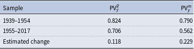
Table 12 reports the change in the post-KW impact output multipliers when changing one parameter at a time. We take the parameter set of the second sample as a benchmark and impose the corresponding values of the first sample, one by one. This decomposition, notwithstanding, produces a numerical error in excess. We also perform the opposite approximation. We take the parameter set of the first sample as a benchmark and impose the corresponding values of the second sample, one at a time. This approximation produces a numerical error by default. Eventually, we calculate the mean values from both approximations. Once the (counterfactual) multipliers have been computed, we present the predicted change in the multiplier. To avoid unnecessary clutter, we only list parameters that generate changes over 0.01 (1 cent).
The bulk of the change in the multipliers is accounted for by a change in household parameters, environmental ratios, and fiscal rules parameters, groups (1a), (2), and (3a), respectively. More concretely, the fall in the consumption habit persistence parameter $\mu$
(from 0.84 to 0.60) can account for 9.0 and 7.8 cents in the defense and nondefense multipliers, respectively. These values represent between one-third and three-quarters of the estimated change in the multipliers. As we highlighted in Table 2, the estimated value of
$\mu$
(from 0.84 to 0.60) can account for 9.0 and 7.8 cents in the defense and nondefense multipliers, respectively. These values represent between one-third and three-quarters of the estimated change in the multipliers. As we highlighted in Table 2, the estimated value of $\mu$
decreased in the post-KW sample, which favors a (more) negative wealth effect response in private consumption and, consequently, a fall in the multiplier.
$\mu$
decreased in the post-KW sample, which favors a (more) negative wealth effect response in private consumption and, consequently, a fall in the multiplier.
The GDP expenditure ratios are extremely relevant for the defense impact output multiplier; the new GDP shares can account for 11.0 cents out of a total decline of 22.9 cents, nearly half of the total change.
The multipliers are also sensitive to the autocorrelation coefficients of public expenditure, $\rho _{g}$
and
$\rho _{g}$
and $\rho _{m}$
. As shown in Table 4, the persistency in the fiscal rules increases in the second sample: from 0.51 to 0.60 for
$\rho _{m}$
. As shown in Table 4, the persistency in the fiscal rules increases in the second sample: from 0.51 to 0.60 for $\rho _{g}$
and from 0.44 to 0.78 for
$\rho _{g}$
and from 0.44 to 0.78 for $\rho _{m}$
.Footnote 18 For the nondefense expenditure multipliers, the increased persistency entails a fall in the multiplier of 1.5 cents; similarly, the defense expenditure multiplier drops by 5.5 cents as a consequence of the higher value of
$\rho _{m}$
.Footnote 18 For the nondefense expenditure multipliers, the increased persistency entails a fall in the multiplier of 1.5 cents; similarly, the defense expenditure multiplier drops by 5.5 cents as a consequence of the higher value of $\rho _m$
. Therefore, the rise in fiscal persistence after the Korean War reduced discretion and increased the wealth effect on consumption, moderating the spending multipliers.
$\rho _m$
. Therefore, the rise in fiscal persistence after the Korean War reduced discretion and increased the wealth effect on consumption, moderating the spending multipliers.
We should add that these findings are consistent with other research studies, such as Fatás and Mihov (Reference Fatás and Mihov2006) or Afonso et al. (Reference Afonso, Agnello and Furceri2010). The latter authors find that tighter fiscal constraints (higher $\rho _{m}$
and
$\rho _{m}$
and $\rho _{g}$
) lead to less discretion (lower
$\rho _{g}$
) lead to less discretion (lower $\sigma _{m}$
) and, consequently, less responsiveness of fiscal policies to output fluctuations (a decline in
$\sigma _{m}$
) and, consequently, less responsiveness of fiscal policies to output fluctuations (a decline in $\theta _{g}^{y}$
). More precisely, lower discretion (alternatively, higher persistence) can generate an ambiguous overall effect on macroeconomic stability. On the one hand, lower discretion limits the ability of the fiscal authority to respond when negative shocks hit, as automatic stabilizers now play a lesser role. On the other hand, a smaller variance of the fiscal rules entails a lower output volatility. The model can reasonably reproduce the moderation occurring after the Korean War (Table 6 vs. Table 7). Following Fatás and Mihov (Reference Fatás and Mihov2006), tighter fiscal constraints after the Korean War led to increasing output stability, though the smaller multipliers limited the government’s ability to affect output through fiscal policy.
$\theta _{g}^{y}$
). More precisely, lower discretion (alternatively, higher persistence) can generate an ambiguous overall effect on macroeconomic stability. On the one hand, lower discretion limits the ability of the fiscal authority to respond when negative shocks hit, as automatic stabilizers now play a lesser role. On the other hand, a smaller variance of the fiscal rules entails a lower output volatility. The model can reasonably reproduce the moderation occurring after the Korean War (Table 6 vs. Table 7). Following Fatás and Mihov (Reference Fatás and Mihov2006), tighter fiscal constraints after the Korean War led to increasing output stability, though the smaller multipliers limited the government’s ability to affect output through fiscal policy.
Table 12. Change in PV multiplier when switching

Under an NK framework, Coenen et al. (Reference Coenen, Erceg, Freedman, Furceri, Kumhof, Lalonde, Laxton, Lindé, Mourougane, Muir, Mursula, de Resende, Roberts, Roeger, Snudden, Trabandt and in’t Veld2012) find that multipliers increase with fiscal persistency, peaking at 3-year persistency and declining thereafter, under the assumption of an accommodative monetary policy. Indeed, for a permanent fiscal expansion (or $\rho _g=1$
in our terms), they find lower multipliers even under an accommodative monetary policy. Actually, the monetary accommodation that they assume does not follow an increase in the (nominal) interest rate, which is held constant. After a fiscal expansion, inflation increases and, in their context, the real interest rate declines, which increases the fiscal multiplier. In our case, by contrast, regardless of the sample period, a positive fiscal shock increases the real interest rate, which exacerbates the crowding-out effect on investment and consumption due to the negative wealth effect.
$\rho _g=1$
in our terms), they find lower multipliers even under an accommodative monetary policy. Actually, the monetary accommodation that they assume does not follow an increase in the (nominal) interest rate, which is held constant. After a fiscal expansion, inflation increases and, in their context, the real interest rate declines, which increases the fiscal multiplier. In our case, by contrast, regardless of the sample period, a positive fiscal shock increases the real interest rate, which exacerbates the crowding-out effect on investment and consumption due to the negative wealth effect.
7.1. Discussion
In summary, the fall in the magnitude of the PV multipliers in the post-KW sample can be accounted for by lower consumption habit persistence, paired with larger autocorrelation coefficients of public expenditure; as we have argued earlier, both of these changes lead to a stronger negative wealth effects on consumption.
As Ramey (Reference Ramey2011) has emphasized, fiscal shocks identified through SVAR tools tend to be partly anticipated, which produces biased estimates of the multiplier. To overcome this problem, Ramey proposes including narrative series of future defense spending in SVAR to control for fiscal news. However, within the context of a DSGE model, despite news has been fairly identified, news about forthcoming fiscal expansions is not much informative about changes in the multiplier. Fiscal news plays an otherwise useful role in another respect: they account for a sizable portion of debt variability at medium-term frequencies, as we illustrate in the variance decomposition.
Figures 9–11 present a sensitivity analysis where we change the range of the key parameters $\{\mu,\chi,\gamma ; \rho _{g},\rho _{m}; \theta _g^m, \theta _g^y, \theta _g^b\}$
, for which the multipliers are sensitive. As in Table 12, we take the parameters estimated for the second sample for granted and compute (ceteris paribus) the output PV multipliers changing the value of these parameters, one at a time. In all figures, shaded areas indicate 95% confidence bands around the post-KW posterior mean.
$\{\mu,\chi,\gamma ; \rho _{g},\rho _{m}; \theta _g^m, \theta _g^y, \theta _g^b\}$
, for which the multipliers are sensitive. As in Table 12, we take the parameters estimated for the second sample for granted and compute (ceteris paribus) the output PV multipliers changing the value of these parameters, one at a time. In all figures, shaded areas indicate 95% confidence bands around the post-KW posterior mean.

Figure 9. Sensitivity analysis of the impact output multiplier.

Figure 10. Sensitivity analysis of the impact output multiplier, fiscal rule autocorrelations.

Figure 11. Sensitivity analysis of the impact output multiplier, nondefense responsiveness.
Figure 9 presents the multiplier sensitivity with respect to household parameters. Consistent with Table 12, the change in these parameters can account for three-quarters of the decline in the multiplier. Figures 10 and 11 present analogous results with respect to fiscal policy parameters $\{\rho _g, \rho _m; \theta _g^m, \theta _g^b,\theta _g^y\}$
. For the persistency parameter
$\{\rho _g, \rho _m; \theta _g^m, \theta _g^b,\theta _g^y\}$
. For the persistency parameter $\rho _m$
, the posterior mean of the pre-KW sample lies well outside the shadowed 95% confidence band area. Given our earlier discussion, the increase in the value of this parameter (which happens at the same time that structural variances decline) helps explain the decrease of fiscal discretion and the decline of the multipliers.
$\rho _m$
, the posterior mean of the pre-KW sample lies well outside the shadowed 95% confidence band area. Given our earlier discussion, the increase in the value of this parameter (which happens at the same time that structural variances decline) helps explain the decrease of fiscal discretion and the decline of the multipliers.
Concerning the remaining fiscal parameters $\{\theta _{g}^{m},\theta _{g}^{b},\theta _{g}^{y}\}$
, panel [a] in Figure 11 shows high sensitivity of the nondefense multiplier with respect to the internal budgetary adjustment: The lower the
$\{\theta _{g}^{m},\theta _{g}^{b},\theta _{g}^{y}\}$
, panel [a] in Figure 11 shows high sensitivity of the nondefense multiplier with respect to the internal budgetary adjustment: The lower the $\theta _{g}^{m}$
, the higher the multiplier response. The slope
$\theta _{g}^{m}$
, the higher the multiplier response. The slope $\Delta \text{PV}_{m}^{y}/\Delta \theta _{g}^{m}$
is negative, while the equivalent for nondefense spending,
$\Delta \text{PV}_{m}^{y}/\Delta \theta _{g}^{m}$
is negative, while the equivalent for nondefense spending, $\Delta \text{PV}_{g}^{y}/\Delta \theta _{g}^{m}$
, remains flat. In other words, the lower the US spending elasticity with respect to military outlays (
$\Delta \text{PV}_{g}^{y}/\Delta \theta _{g}^{m}$
, remains flat. In other words, the lower the US spending elasticity with respect to military outlays ( $\theta _{g}^{m}$
), the higher the effectiveness of fiscal policy is. To the best of our knowledge, this channel of internal adjustment has not been explored before.
$\theta _{g}^{m}$
), the higher the effectiveness of fiscal policy is. To the best of our knowledge, this channel of internal adjustment has not been explored before.
Finally, panels [b] and [c] in Figure 11 show that the nondefense expenditure multipliers are flat with respect to the debt and output response parameters. This contrasts with the results of Leeper et al. (Reference Leeper, Plante and Traum2010), Ilzetzki et al. (Reference Ilzetzki, Mendoza and Végh2013), and Zubairy (Reference Zubairy2014), who provide evidence that the multipliers are remarkably sensible to $\theta _g^b$
and
$\theta _g^b$
and $\theta _g^y$
.
$\theta _g^y$
.
Coenen et al. (Reference Coenen, Erceg, Freedman, Furceri, Kumhof, Lalonde, Laxton, Lindé, Mourougane, Muir, Mursula, de Resende, Roberts, Roeger, Snudden, Trabandt and in’t Veld2012) document that the multipliers tend to be higher in the USA than in Europe, using a wide variety of NK models. They conclude that these differences are due to the different degree of openness in European economies relative to the US economy. Our model assumes a closed economy, which entails a larger multiplier relative to an open economy setting. Other aspects, such as the degree of nominal rigidities or the role of automatic stabilizers—which tend to be higher for Europe than the USA and could help account for the lower multipliers in Europe—play a much lesser role to account for the difference in the multipliers. As documented in Table 4, the automatic stabilizer parameter $\theta _g^y$
decreases to 0.060 (from a high of 0.089) in our estimation. In this context, our multiplier estimates fall, not rise. And even if this parameter were to increase, the results shown in Figure 11[b] show that large movements in
$\theta _g^y$
decreases to 0.060 (from a high of 0.089) in our estimation. In this context, our multiplier estimates fall, not rise. And even if this parameter were to increase, the results shown in Figure 11[b] show that large movements in $\theta _g^y$
generate small changes in the multiplier.
$\theta _g^y$
generate small changes in the multiplier.
8. Concluding remarks
In this paper, we have documented a permanent fall in the magnitude of the US multiplier that occurred after the Korean War. To analyze this decline, we have estimated a DSGE model using Bayesian techniques and a long-run yearly series that explicitly accounts for defense and nondefense news shocks. We conclude that the effectiveness of spending policies—as measured by the expenditure multiplier—has decreased in the post-KW sample due to changes in preferences and policy choices—from 0.82 to 0.71 in nondefense and 0.79 to 0.56 in defense spending.
The decline in the value of the multiplier can be linked to changes in two model parameters: a fall in the consumption habit persistence ( $\mu$
), paired with a rise in the persistence of the public expenditure processes (
$\mu$
), paired with a rise in the persistence of the public expenditure processes ( $\rho _m$
and
$\rho _m$
and $\rho _g$
). Other fiscal parameters—which earlier research papers have shown to be relevant, such as those linking expenditure with the state of debt (
$\rho _g$
). Other fiscal parameters—which earlier research papers have shown to be relevant, such as those linking expenditure with the state of debt ( $\theta _{b}^{g}$
) or automatic stabilizers (
$\theta _{b}^{g}$
) or automatic stabilizers ( $\theta _{y}^{g}$
)—have not affected the magnitude of the fiscal multiplier in the USA. That said, the role of the budgetary adjustment parameter
$\theta _{y}^{g}$
)—have not affected the magnitude of the fiscal multiplier in the USA. That said, the role of the budgetary adjustment parameter $(\theta _{m}^{g})$
might be relevant, though the observed decline in the multiplier should not be associated with it.
$(\theta _{m}^{g})$
might be relevant, though the observed decline in the multiplier should not be associated with it.
When the model is estimated without news, we find that the model properly identifies anticipated military spending—as compared to Ramey’s (Reference Ramey2009) narrative series—yet the inclusion of news is irrelevant to the change in the multiplier. Notwithstanding, a variance decomposition exercise illustrates that fiscal news accounts for the bulk of the variances of debt and defense expenditures at medium-term frequencies. This is a relevant point, to the extent that high debt levels reduce fiscal effectiveness as deeper fiscal tightening will be required in the near future [see Ilzetzki et al. (Reference Ilzetzki, Mendoza and Végh2013)].
Complementarily, we have also documented a decline in the variability of news about future fiscal expenditure; that is, fiscal policies are now better anticipated than during 1939–1955, a period that involved two important warfare episodes. The pattern of fiscal news, on the other hand, has been fairly identified by the model, as compared with the narrative series proposed by Ramey (Reference Ramey2011). However, we have identified some episodes of discrepancy between our DSGE model’s news prediction and those narrative provided by Ramey, which calls for further effort to reconcile both approaches.
The debate about the effectiveness of fiscal policy has increased over the last decade, especially in the aftermath of the Great Recession and, almost a decade later, the COVID–19 crisis and the war in Ukraine. Although the origins of these episodes are different, the usefulness of fiscal tools to cope with these crises depends on their ability to affect output. Under the lens of our model, these changes in fiscal scenarios have reduced the degree of discretion and, thereby, increased the role of fiscal rules. Put differently, our conclusion points out that the role of discretionary increases in government spending to boost output has declined at all time horizons.
Appendix A
A.1. Data and sources
The estimation procedure considers nine observable variables. We include consumption, investment, defense and nondefense government expenditure, transfers, tax rates on capital income, labor income, and consumption, and debt outstanding.
The first four series come from the Bureau of Economic Analysis (BEA). Since we want to incorporate observations that include WWII, our analysis is limited to annual series; quarterly series are provided by the BEA from 1947 to present only.
-
• Consumption ( $C$
) is defined as the sum of nondurable goods consumption and services consumption,
$\text{CNonDur}+ \text{CServ}$
(Table 1.1.5, lines 5 and 6).
$C$
) is defined as the sum of nondurable goods consumption and services consumption,
$\text{CNonDur}+ \text{CServ}$
(Table 1.1.5, lines 5 and 6). -
• Investment (
$X$
) is defined as the sum of durable goods consumption and fixed investment,
$\text{CDur}+\text{FI}$
(Table 1.1.5, lines 4 and 8). -
• Total government expenditure consists of (federal-level) defense government expenditure and (federal, state, and local) nondefense government expenditure. In turn, defense government expenditure (
$M$
) is retrieved from Table 1.1.5, line 24, while nondefense expenditure (
$G$
) consists of federal spending plus state and local public expenditure (Table 1.1.5, lines 25 and 26). -
• Transfers (
$\tau$
) are obtained from the series A577RC1A027NBEA, personal current transfer receipts, from the St. Louis Fed’s FRED database. -
• Regarding consumption, labor income, and capital income tax rates, we follow the methodology of Mendoza et al. (Reference Mendoza, Razin and Tesar1994), who derive aggregate estimates for effective tax rates using national accounts. [Both Leeper et al. (Reference Leeper, Plante and Traum2010) and Fernández-Villaverde et al. (Reference Fernández-Villaverde, Guerrón-Quintana, Kuester and Rubio-Ramírez2015) calculate tax rates with a similar strategy.] The consumption tax rate (
$\tau _c$
) is computed as the sum of Excise taxes,
$\text{ExcT}$
, Customs duties,
$\text{CustDut}$
, and Sales taxes,
$\text{SalesT}$
(Table 3.2, lines 5, 6, and 7), divided by the sum of Personal consumption expenditures
$C$
(Table 1.1.5, line 2) and government consumption expenditures
$G+M$
(Table 3.9.5, line 2):
\begin{equation*} \tau _{c}=\frac {\text{ExcT}+\text{CustDut}+\text{SalesT}}{C+( G+M) }. \end{equation*}
The income tax rate
$\tau _Y$
—which is not used directly as an observable variable—is calculated as the ratio of Income tax revenues
$\text{IncT}$
(Table 3.4, lines 3 and 9) over the sum of Proprietors’ income with inventory valuation and capital consumption adjustments (PI, Table 2.1, line 9), Rental income of persons with capital consumption adjustment (RICCA, Table 2.1, line 12), Personal income receipts on assets (PIRA, Table 2.1, line 13), Wages and salaries (
$W$
), and Supplements to wages and salaries (SW) (Table 2.1, lines 3 and 6):Using the calculated tax rate on income
\begin{equation*} \tau _{Y}=\frac {\text{IncT}}{\text{PI}+\text{RICCA}+\text{PIRA}+( W+\text{SW}) }. \end{equation*}
$\tau _{Y}$
, the tax rate on labor income (
$\tau _{n}$
) iswhere GSI denotes Contributions for government social insurance (Table 3.1, line 7), and CE denotes Compensation to employees (Table 2.1, line 2). Finally, the tax rate on capital income (
\begin{equation*} \tau _{n}=\left ( \tau _{Y}+\frac {\text{GSI}}{W+\text {SW}}\right ) \frac {W+\text{SW}}{\text{CE}}, \end{equation*}
$\tau _k$
) is computed as:where PT denotes Property taxes (Table 3.4, line 11), TCI denotes taxes on corporate income (Table 3.2, line 7; Table 3.3, line 10), and IRA denotes Income receipts on assets (Table 4.1, line 9).
\begin{equation*} \tau _{k}=\frac {\tau _{Y}( \text{PI}+\text{RICCA}+\text {PIRA}) +\text{PT}+\text{TCI}}{\text{PI}+\text{PIRA}+\text{IRA}}, \end{equation*}
-
The dollar amount of debt
$b$
is obtained from the Historical Debt Outstanding statistics found in the Treasury Direct website.


A.1.1. Observable variables
All series (except for tax rates) are transformed into real, per-capita series by dividing by the GDP implicit deflator (Table 1.1.4, line 1) and midyear population (Table 2.1, line 40). Once we do this, all series described above are logged and regressed against a constant and linear, quadratic, and cubic time trends. The residuals are the observable variables we use in the econometric analysis.
Figure 12 presents the six observable variables in levels (consumption, investment, defense and nondefense expenditure, transfers, and debt outstanding) for the first sample (1939–1954). Figure 13 does the same for the second sample (1955–2017). Finally, Figure 14 presents our estimates for the three observable variables in percentages (labor income, capital income, and consumption tax rates), as well as the debt-to-output ratio.

Figure 12. Observable variables in levels, 1939–1954.

Figure 13. Observable variables in levels, 1955–2017.

Figure 14. Selected fiscal variables, 1939–2017.
A.2. Equilibrium conditions
Given the model economy described in the paper, let $\lambda _{t}$
denote the Lagrange multiplier on the budget constraint that results from merging equations (3) and (4) and
$\lambda _{t}$
denote the Lagrange multiplier on the budget constraint that results from merging equations (3) and (4) and $\xi _{t}$
be the multiplier associated with the law of motion for capital (5). Then, the first-order conditions that characterize the economy’s equilibrium are as follows:
$\xi _{t}$
be the multiplier associated with the law of motion for capital (5). Then, the first-order conditions that characterize the economy’s equilibrium are as follows:
 \begin{align} \lambda _{t}(1+\tau _{ct}) = & \ q_{t}^{-1}-\beta \mu E_{t}q_{t+1}^{-1} \end{align}
 \begin{align} \lambda _{t} &= \xi _{t}-\xi _{t}S^{\prime }\bigg (\frac{x_{t}}{x_{t-1}}\bigg )\frac{x_{t}}{x_{t-1}}-\xi _{t}S\bigg (\frac{x_{t}}{x_{t-1}}\bigg ) \nonumber\\ &\quad + \beta E_{t}\xi _{t+1}S^{\prime }\bigg (\frac{x_{t+1}}{x_{t}}\bigg )\bigg (\frac{x_{t+1}}{x_{t}}\bigg )^{2} \end{align}
 \begin{align} \lambda _{t}(1-\tau _{nt})w_{t} = & \ \phi n_{t}^{\chi } \end{align}
 \begin{align} \lambda _{t}(1-\tau _{kt})r_{t} &= -\lambda _{t}\delta ^{\prime }(u_{t})\tau _{kt}+\xi _{t}\delta ^{\prime }(u_{t}) \end{align}
 \begin{align} \xi _{t} &= \beta E_{t}\lambda _{t+1}(1-\tau _{k,t+1})r_{t+1}u_{t+1} \nonumber\\ &\quad + \beta E_{t}\lambda _{t+1}\delta (u_{t+1})\tau _{k,t+1}+\beta E_{t}\xi _{t+1} -\,\beta E_{t}\xi _{t+1}\delta (u_{t+1}) \end{align}
 \begin{align} \lambda _{t} = & \ \beta E_{t}\lambda _{t+1}r_{t}^{b} \end{align}
 \begin{align} k_{t+1} = & \ k_{t}-\delta (u_{t})k_{t}+x_{t}-x_{t}S\bigg (\frac{x_{t}}{x_{t-1}}\bigg ) \end{align}
 \begin{align} y_{t} = & \ z_{t}(u_{t}k_{t})^{\alpha }n_{t}^{1-\alpha } \end{align}
 \begin{align} \alpha y_{t} = & \ r_{t}u_{t}k_{t} \end{align}
 \begin{align} (1-\alpha )y_{t} = & \ w_{t}n_{t} \end{align}
 \begin{align} g_{t}+m_{t}+r_{t-1}^{b}b_{t-1}+\tau _{t} = & \ b_{t}+\tau _{ct}c_{t}+\tau _{kt}r_{t}u_{t}k_{t}+\tau _{nt}w_{t}n_{t} - \delta (u_{t})\tau _{kt}k_{t} \end{align}
 \begin{align} y_{t} = & \ c_{t}+x_{t}+g_{t}+m_{t} \end{align}
 \begin{align} q_{t} = & \ c_{t}-\mu c_{t-1}. \end{align}
In the above, equations (19)–(24) are the household’s first-order conditions with respect to the decision variables $\{c,x,n,u,k,b\}$
, (25) is the law of motion for capital, equations (26)–(28) characterize the firm’s profit maximization problem, (29) is the government’s budget constraint, (30) is the aggregate feasibility constraint, and (31) adds an auxiliary variable that is used to simplify the household’s first-order condition (19).
$\{c,x,n,u,k,b\}$
, (25) is the law of motion for capital, equations (26)–(28) characterize the firm’s profit maximization problem, (29) is the government’s budget constraint, (30) is the aggregate feasibility constraint, and (31) adds an auxiliary variable that is used to simplify the household’s first-order condition (19).
A.3. Estimation details
For each preference specification/sample period combination, we run two chains of 20 million replications, using the first 15 million as a burn-in. Our acceptance rates are in the neighborhood of 0.25, as shown in Table 13.
Table 13. Acceptance ratios


