


1. Introduction
The mean velocity distribution in the outer part of a turbulent boundary layer is often expressed as a combination of a logarithmic part and a wake component, as in
 \begin{equation} \frac{U}{u_\tau} = \frac{1}{\kappa} \ln{\frac{yu_\tau}{\nu}} +B + \frac{2\varPi}{\kappa} W \left( \frac{y}{\delta} \right), \end{equation}
where  $U$ is the mean velocity in the streamwise direction, $u_\tau = \sqrt {\tau _w/\rho }$, $\tau _w$ is the shear stress at the wall where $y=0$, $\rho$ is the fluid density, $\kappa$ is von Kármán's constant, $B$ is the additive constant and $\varPi$ is the Reynolds-number-dependent wake factor. The wake function $W$ is taken to be a universal function of $y/\delta$, where $\delta$ is the outer layer length scale. This wall-wake model was first formulated by Coles (Reference Coles1956), and it is an essential part of the widely used composite profile derived by Chauhan, Nagib & Monkewitz (Reference Chauhan, Nagib and Monkewitz2007).
Marusic, Uddin & Perry (Reference Marusic, Uddin and Perry1997) proposed a similar formulation for the streamwise turbulence intensity in zero pressure gradient turbulent boundary layers, given by
 \begin{equation} \overline{u^2}^+= B_1 - A_1 \ln \frac{y}{\delta_m} - V_g \left( y^+, \frac{y}{\delta_m} \right) -W_g \left(\frac{y}{\delta_m} \right), \end{equation}
where  $\overline {u^2}^+ = \overline {u^2}/u_\tau ^2$. The model incorporates the log-law for $\overline {u^2}^+$ with constants $A_1$ and $B_1$ (Hultmark et al. Reference Hultmark, Vallikivi, Bailey and Smits2012; Marusic et al. Reference Marusic, Monty, Hultmark and Smits2013), where $V_g$ is a mixed scale viscous deviation term, $W_g$ is the wake deviation term and $\delta _m$ is a boundary layer thickness defined in a way that is similar to the Rotta–Clauser thickness. It is typically 15 % to 20 % larger than $\delta _{99}$, the 99 % thickness (further details are given in Appendix A). The wake deviation was given by
 \begin{equation} W_g = B_1 \eta^2(3-2 \eta)- A_1 \eta^2 (1-\eta)(1-2\eta), \end{equation}
where  $\eta =y/\delta _m$. A more recent and simpler version of $V_g$ was given by Baars & Marusic (Reference Baars and Marusic2020) as
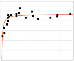
 \begin{equation} V_g = K_1 - K_2/ \sqrt{y^+}, \end{equation}
with  $K_1=4.01$, $K_2=10.13$.
Pirozzoli & Smits (Reference Pirozzoli and Smits2023) proposed an alternative model for the mean velocity distribution in the outer layer, given by a compound logarithmic–parabolic distribution of the type first suggested by Hama (Reference Hama1954); that is,
 $$\begin{gather} \frac{U_e-U}{u_\tau} = B' - \frac{1}{k_0} \ln \frac{y}{\delta_0}, \end{gather}$$
 $$\begin{gather}\frac{U_e-U}{u_\tau} = C \left( 1 - \frac{y}{\delta_0} \right)^2, \end{gather}$$
where  $C$ is a constant, and $U_e$ is the free stream velocity. Requiring the two velocity distributions to smoothly connect up to the first derivative yields the position of the matching point ( $\eta _0=y_0/\delta _0$) and the additive constant $B'$ in (1.5) as a function of $k_0$ and $C$,
$C$,
 \begin{equation} \eta_0 =\frac{1}{2} \Bigg( 1 - \left( 1 - \frac{2 }{C k_0} \right)^{1/2}\Bigg), \quad B' = C (1-\eta_0)^2 + \frac{1}{k_0} \ln \eta_0. \end{equation}
The matching point  $\eta _0$ marks the outer limit of the logarithmic part, (1.5), and the inner limit of the wake part, (1.6). By comparing (1.1) with this compound model, and adopting Coles's wake function which has a maximum at $y/\delta _{99}=1$, we find that $B'=2\varPi /\kappa$, so that $B'$ and $\varPi$ are synonymous with each other. In what they called the classical case, Pirozzoli & Smits (Reference Pirozzoli and Smits2023) found that with $\delta _0=1.6 \delta _{95}$ the best fit of the data was obtained with $k_0 = \kappa \approx 0.38$, $C \approx 9.88$, so that $B'=2.15$, with the two distributions smoothly matched at $\eta _0=0.158$. This compound logarithmic–parabolic distribution fits the velocity distributions well down to $y/\delta _0 \approx 0.01$ (for Reynolds numbers based on displacement thickness greater than 2000).
Here, we suggest a similar approach for the streamwise component of the turbulent stress. That is, we propose a compound representation given by
 $$\begin{gather} \overline{u^2}^+= B_1 - A_1 \ln \frac{y}{\delta_1} , \end{gather}$$
 $$\begin{gather}\overline{u^2}^+= b_1-a_1 \frac{y}{\delta_1} , \end{gather}$$
where  $a_1$ and $b_1$ are constants, and $\delta _1$ is the appropriate length scale for the outer layer. In this formulation, there is no viscous deviation term. Requiring the two turbulence distributions to smoothly connect up to the first derivative yields the position of the matching point ( $\eta _1=y_1/\delta _1$) and the additive constant $B_1$ in (1.8) as a function of the other constants,
 \begin{equation} \eta_1 = \frac{A_1}{a_1}, \quad B_1 = b_1-A_1 (1-\ln{\eta_1}). \end{equation}
The matching point  $\eta _1$ marks the outer limit of the logarithmic part, (1.8), and the inner limit of the wake part, (1.9). According to (1.9), $\overline {u^2}^+$ is zero when $y/\delta _1=b_1/a_1$, and so we impose one further constraint and set $b_1/a_1=1.05$ (which closely corresponds to the point where $y/\delta _{995} = 1$). Finally, if we assume $A_1$ is a true constant ( $=1.26$ for boundary layers according to Marusic et al. (Reference Marusic, Monty, Hultmark and Smits2013)), the only free parameter in our fit to the turbulence profile is $B_1$, which we will show to be a Reynolds-number-dependent turbulence wake factor that behaves similarly to that of the mean velocity wake factor $B'=2\varPi /\kappa$.
2. Comparisons with data
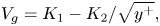
We now demonstrate the quality of the model by comparing it with experimental and direct numerical simulation data over a wide range of Reynolds numbers (see table 1). Before proceeding, we need to specify the particular length scale  $\delta _1$ used to describe the outer layer. We have chosen $\delta _1=\delta _{99}$, for reasons made clear in Appendix A. We also need to relate $Re_\theta =\theta U_e/\nu$, where $\theta$ is the momentum thickness, to the friction Reynolds number $Re_\tau =\delta _{99}u_\tau /\nu$, in that not all data sets specify both. This issue is also addressed in Appendix A.
Table 1. Data sources and fitting parameters for  $A_1=1.26$. Here $B_1$ is the only free parameter, and $b_1$ and the matching point $\eta _1$ are defined by (1.10a,b).
To begin the analysis, we use the data by Samie et al. (Reference Samie, Marusic, Hutchins, Fu, Fan, Hultmark and Smits2018) ( $6250 < Re_\theta < 47\,100$). Figure 1 demonstrates that, as expected from previous work, the logarithmic part with $A_1=1.26$ and $B_1=2.00$ is a good fit in the overlap region. In addition, the linear part of the model describes the profile beyond the matching point very well over this range of Reynolds numbers, except for the region $y/\delta _{99}> 1$ where a more gradual decline is observed. At the highest Reynolds numbers, the compound formulation represents the data well for 95 % of the profile.
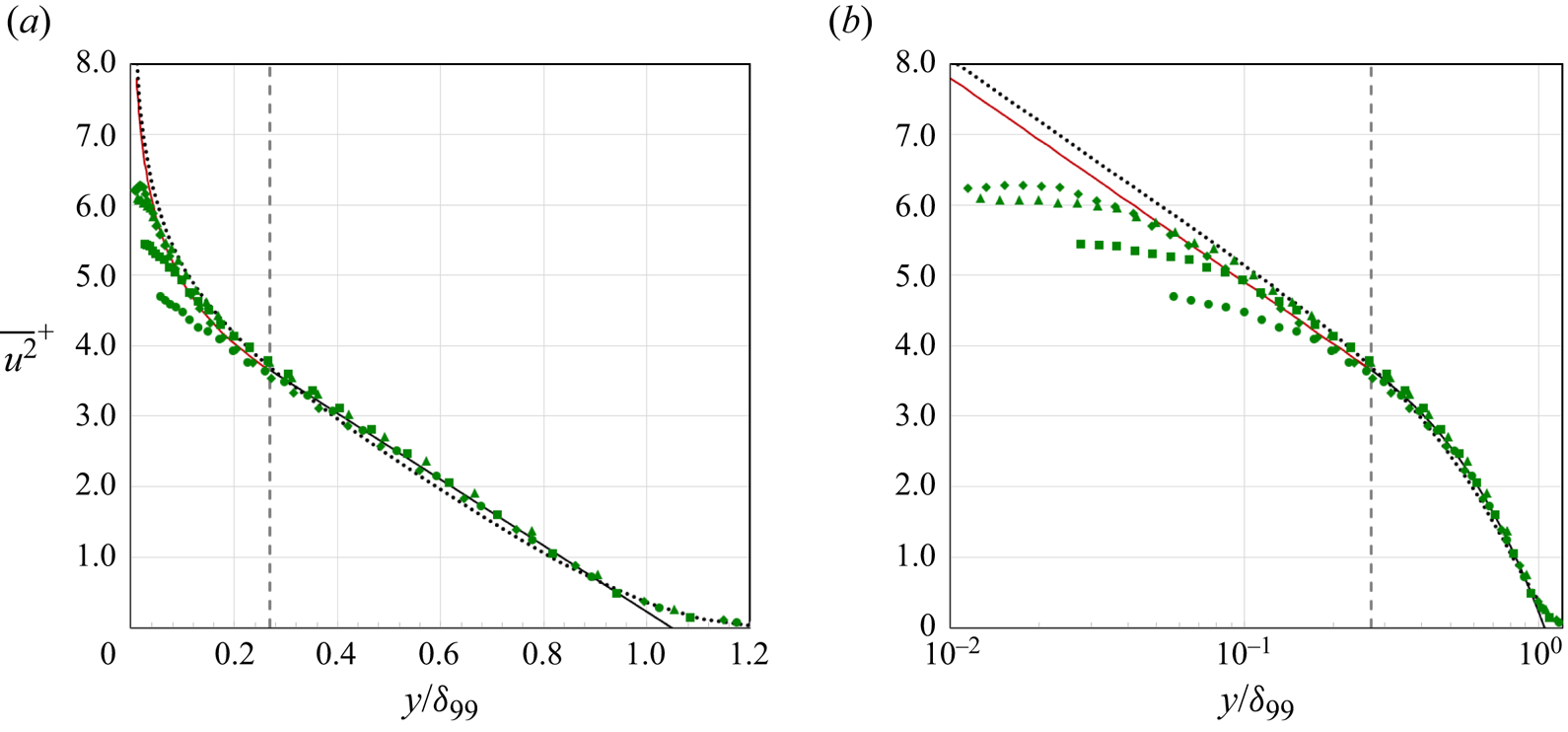
Figure 1. Comparison with the experimental data of Samie et al. (Reference Samie, Marusic, Hutchins, Fu, Fan, Hultmark and Smits2018) for  $Re_\theta =6252\unicode{x2013}47\,096$ ( $y^+>100$, $A_1=1.26$, $B_1=2.00$): (a) linear scaling; (b) logarithmic scaling. Here $\cdots \cdots$, black, (1.2) (neglecting $V_g$); ———, red, (1.8); ———, black, (1.9) (matched at $\eta _1=0.269$, vertical dashed line). Symbols as in table 1.
For reference, we also plot (1.2) for the same values of  $A_1$ and $B_1$ (using $\delta _{99}/\delta _m=0.81$). We neglected the viscous deviation term $V_g$, which leads to a small positive offset of $\overline {u^2}^+$ in (1.2) with respect to the compound formulation in the logarithmic region. Both fits work well beyond the logarithmic region, although it could be argued that the linear fit is a trifle more accurate for $0.2< y/\delta _{99}<0.9$. In the analysis going forward, we will use the compound fit, primarily because the viscous deviation term in (1.2) appears to obscure some of the underlying trends as well as the comparisons between the turbulence and mean velocity profiles.
We now consider all the high-Reynolds-number data listed in table 1 over the range  $6000 \le Re_\theta < 60\,000$. The results are shown in figure 2 for $B_1=2.00$. Although there is some the scatter in the data, the compound fit works reasonably well using this value. The agreement can be improved by using values of $B_1$ optimized for each profile, as listed in table 1.


The low-Reynolds-number data ( $Re_\theta \le 6040$) are shown in figure 3. The compound fit is plotted for two cases, $B_1=2.00$ (the value used for the high-Reynolds-number data shown in figures 1 and 2), and $B_1=1.05$ (chosen to match the lowest-Reynolds-number profile in the data set). In order to match the in-between Reynolds number cases, $B_1$ was varied as given in table 1. Again, we see a very satisfactory fit to the data, even in this low-Reynolds-number range.
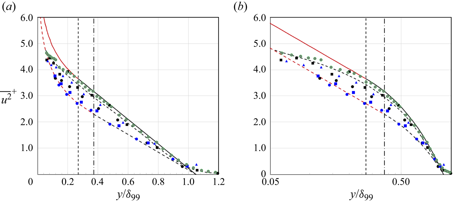
Figure 3. Comparison with the experimental data for  $Re_\theta \le 6040$ ( $y^+>100$): (a) linear scaling; (b) logarithmic scaling. Here ———, black, (1.9); ———, red, (1.8). Here $b_1=4.92$, distributions matched at $\eta _1=0.269$ (vertical dashed line). Here - - - - -, black, (1.9); - - - - -, red, (1.8). Here $b_1=3.56$, distributions matched at $\eta _1=0.372$ (vertical dashed-dotted line). Symbols as in table 1
The constant  $B_1$ appears to act as a wake function for the turbulence profile, similar to the wake function $\varPi$ for the mean velocity profile. In figure 4, we compare the Reynolds number dependence of $B_1$ with that of $2\varPi /\kappa$ (using $\kappa =0.384$, where $B_1$ was scaled by an arbitrary factor of 1.15 to aid the comparison. We see a clear similarity in the behaviour of the two wake functions, in that they increase with Reynolds number up to $Re_\theta \approx 6000$, and then become constant at higher Reynolds numbers.
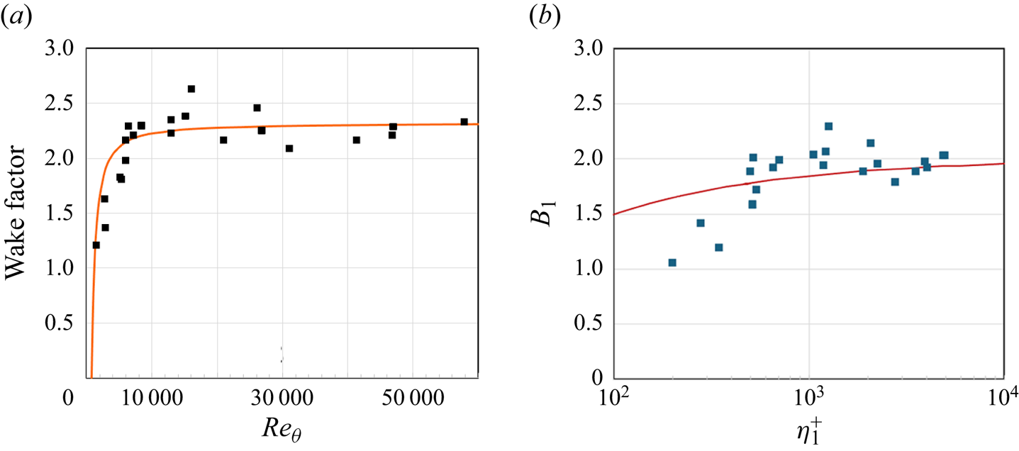
Figure 4. (a) Wake factors versus  $Re_\theta$. Here $\blacksquare$, black, 1.15 $B_1$; ———, red, $B'=2 \varPi /\kappa$ (Chauhan et al. Reference Chauhan, Nagib and Monkewitz2007). (b) Turbulence wake factor $B_1$ as a function of $\eta _1^+$. Red line is $2V_g$ evaluated at $\eta _1^+$ (1.4).
To investigate this connection further, we first consider the wake factor  $B'=2\varPi /\kappa$ for the mean velocity. Now, $B'$ is usually measured as the maximum deviation of the mean velocity profile from the log-law. For high-Reynolds-number flows ( $Re_\theta >6000$, $Re_\tau >1800$), this gives a constant value, as seen in figure 4. However, at low Reynolds numbers ( $Re_\tau \lnapprox 1300$), the log-law ceases to exist and it is replaced by a power law (Zagarola & Smits Reference Zagarola and Smits1998a,Reference Zagarola and Smitsb), and $B'$ begins to decrease. It is suggested here that the decrease in $B'$ at low Reynolds numbers is a result of incorrectly using a log-law to measure it at Reynolds numbers where no log-law exists.
As for the turbulence, the wake factor  $B_1$ is the offset of the turbulence profile from its logarithmic variation. At high Reynolds numbers, $B_1$ is a constant, as seen in figure 4, but for $Re_\tau \lnapprox 2000$ the turbulence log-law (with constant $A_1$ and $B_1$) is usually assumed to vanish (Hultmark et al. Reference Hultmark, Vallikivi, Bailey and Smits2012; Marusic et al. Reference Marusic, Monty, Hultmark and Smits2013). However, when we allow $B_1$ to vary with Reynolds number, we see that a logarithmic variation in the turbulence appears to be maintained, even at low Reynolds numbers.
This Reynolds number dependence of  $B_1$ suggests that there may be a link to the viscous deviation term $V_g$, (1.4), in that they both embody the effects of viscosity. One way to explore this connection is to see how $B_1$ varies with $\eta _1^+=\eta _1 u_\tau /\nu$ (see table 1). From figure 1, we see that $B_1$ begins to decrease quite sharply for $\eta _1^+ < 500$. We also show the value of $V_g$ (as given by Baars & Marusic (Reference Baars and Marusic2020)) at the matching point, and the trend in B1 is noticeably more severe than that of $V_g$.
We suggest, therefore, that the similarity between the Reynolds number dependence of  $B'$ and $B_1$ is a direct result of changes in the scaling behaviour of the mean velocity and turbulence profiles at low Reynolds number. In the first case, the log-law is replaced by a power law, and in the second case the slope of the logarithmic behaviour $A_1$ appears to remain constant while its intercept $B_1$ decreases. In that $A_1$ remains constant, it would indicate that the turbulence continues to obey the attached eddy scaling of $y^{-1}$, even at low Reynolds numbers (see Smits (Reference Smits2022) for further details).
3. Conclusions and discussion
The logarithmic–linear compound fit in  $y/\delta _{99}$ proposed here for the streamwise turbulent stress $\overline {u^2}^+$ in the outer layer of a turbulent boundary layer works well over a wide range of Reynolds numbers. For the logarithmic part of the fit we assumed that $A_1$, the slope of the log-law, is fixed at 1.26 (as given by Marusic et al. (Reference Marusic, Monty, Hultmark and Smits2013)), and the linear part of the fit was constrained to pass through zero at $y/\delta _{99}=1.05$. As a consequence, the fit has only one free parameter, $B_1$, which acts like a wake factor.
For low Reynolds numbers ( $Re_\theta \le 6040$), $B_1$ increases with increasing Reynolds number, attaining an approximately constant value of approximately 2 for high Reynolds numbers ( $6000 \le Re_\theta \le 60\,000$). At low Reynolds numbers ( $Re_\theta < 6000$), $B_1$ decreases with decreasing Reynolds number. The behaviour of $B_1$ with Reynolds number closely follows the variation of the mean flow wake factor $B'=2\varPi /\kappa$, and we propose that this is a direct result of changes in the scaling behaviour of the mean velocity and turbulence profiles at low Reynolds number: for the mean velocity the log-law is replaced by a power law, and for the turbulence the log-law intercept is Reynolds number dependent while it continues to obey the attached eddy wall-normal dependence.
For the logarithmic parts of the mean velocity and the turbulence distributions, we know that we can connect the behaviour of  $B'$ and $B_1$ through the attached eddy hypothesis (Perry & Chong Reference Perry and Chong1982; Marusic & Monty Reference Marusic and Monty2019). For the parabolic part of the mean velocity, (1.6), and the linear part of the turbulence, (1.9), the link is still unknown. One possibility is to consider the behaviour of the ‘detached’ (or Type B) eddies (Perry & Marusic Reference Perry and Marusic1995). However, as they note, building this connection ‘would be very complicated and would depend on the assumed shape of the representative eddies’. Also, as Hu, Yang & Zheng (Reference Hu, Yang and Zheng2020) point out, ‘unlike the attached eddies, whose statistical behaviours are well described by the (attached eddy hypothesis), the detached eddies lack a good phenomenological model’. Building a better understanding of the physics that connects the mean velocity and the turbulence in the outer layer is clearly in need of further work.
Acknowledgements
The authors would like to thank S. Pirozzoli and J.-P. Dussauge for their comments on an earlier draft.
Declaration of interests
The author reports no conflict of interest.
Appendix A. Data analysis
For the length scale used to describe the outer layer,  $\delta _1$, there are a multitude of choices. In examining the mean flow, Pirozzoli & Smits (Reference Pirozzoli and Smits2023) considered $\delta _0=1.6 \delta _{95}$, $0.28 \varDelta$ and $2\delta _N$, where $\varDelta =(U_e/u_\tau )\delta ^*$ is the Rotta–Clauser thickness, $\delta ^*$ is the displacement thickness, $\delta _N=(H/(H-1))\delta ^*$ and $H=\delta ^*/\theta$ is the shape parameter. For the data in table 1, Sillero et al. (Reference Sillero, Jiménez and Moser2013), DeGraaff & Eaton (Reference DeGraaff and Eaton2000) and Vallikivi et al. (Reference Vallikivi, Hultmark and Smits2015) used $\delta _{99}$, Osaka et al. (Reference Osaka, Kameda and Mochizuki1998) used $\delta _{995}$, and Samie et al. (Reference Samie, Marusic, Hutchins, Fu, Fan, Hultmark and Smits2018) used $\delta _{c}$, where $\delta _c$ is the outer length scale adopted by Chauhan et al. (Reference Chauhan, Nagib and Monkewitz2007) for their composite profile. In order to compare data, we need a common standard, and we will show that $\delta _1=\delta _{99}$ serves that purpose well. To convert $\delta _{995}$ and $\delta _c$ to the matching value of $\delta _{99}$, we used the composite profile. In figure 5, we show how these various thicknesses compare.
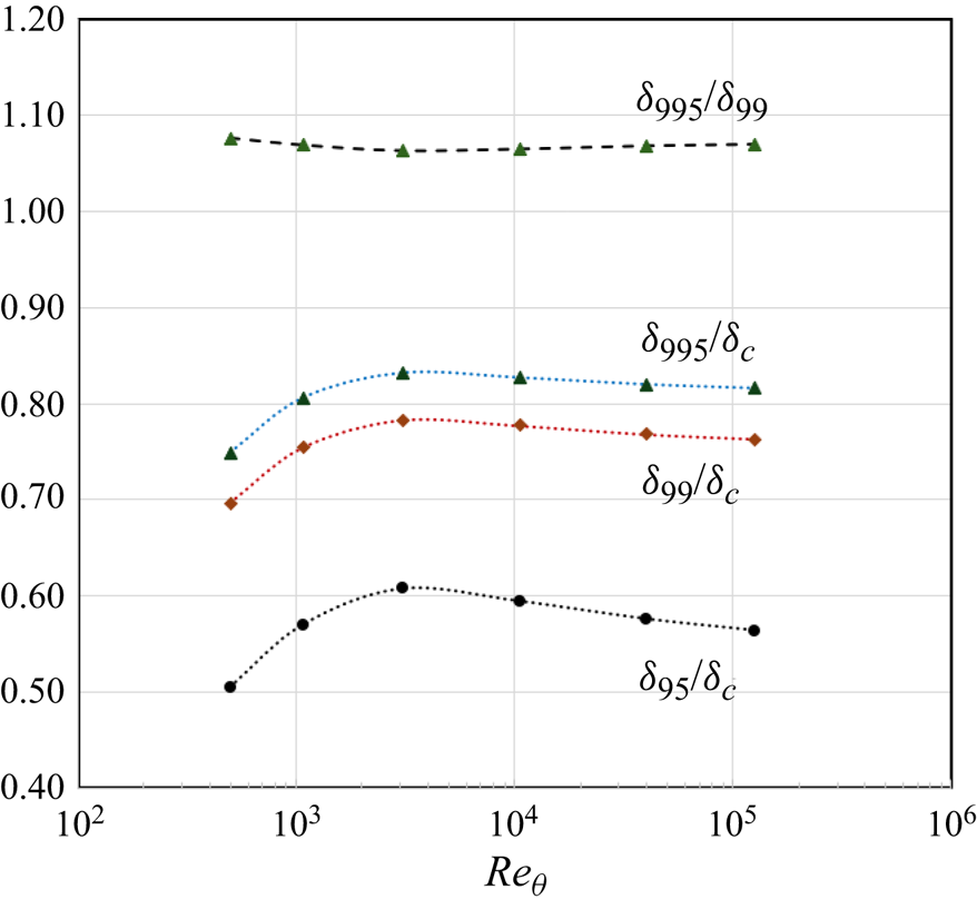
Figure 5. Boundary layer thickness variations with  $Re_\theta$, as found using the composite profile (Chauhan et al. Reference Chauhan, Nagib and Monkewitz2007).
We used the results of Klebanoff (Reference Klebanoff1955) on the eddy viscosity. His boundary layer thickness was approximately 1.15 times larger than  $\delta _{99}$ (Smits Reference Smits2024), and the data were scaled accordingly.
In addition, we need to relate  $Re_\theta$ and $Re_\tau$, in that not all data sets specify both. Here, we use
 \begin{equation} Re_\theta = 3.241 Re_\tau, \end{equation}
based on a fit to the available data ( $R^2=0.9997$ for full data set), see figure 6.
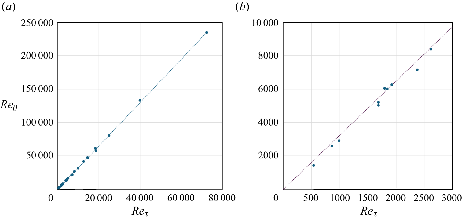
Figure 6. Momentum thickness Reynolds number versus friction Reynolds number: dashed line, (A1); (a) full data set; (b) data for  $Re_\theta < 10\,000$.
Finally, the  $Re_\theta =234\,670$ profile by Vallikivi et al. (Reference Vallikivi, Hultmark and Smits2015) was corrected for an error in the 99 % thickness, which was smaller by a factor of 0.943 than the value originally reported. This changed the profile, and the corresponding value of $Re_\tau$. Also, the Fernholz profile at $Re_\theta =21\,410$ was not used since it has some obvious problems.


 Open access