


In response to the public finance challenges posed by population ageing, governments across the developed world have been legislating for increases in the ages at which public pensions can be received. The impact of these reforms on the public finances – and on household incomes – will depend not only on the generosity of typical public pension payments but also on how private incomes respond – for example, due to changes in labour supply – and the operation of the rest of the personal tax and benefit system.
The direct impact of delayed public pension income receipt on household incomes may be mitigated if public pension income is taxable, if private incomes – such as earnings – increase in response to a rise in the pension age, or if other state transfers or benefits – perhaps targeted at those with low incomes or those in poor health – are available to replace some of the public pension income forgone. But these potential knock-on effects will also have different consequences for the public finances: if taxable private incomes increase, the public finances would tend to be strengthened further; conversely, if household incomes are cushioned by reduced tax payments or increased benefit income, the gains to the public finances from delayed public pension payments would be offset.
In 1995, the United Kingdom (UK) government legislated to increase the early retirement age (ERA) – the earliest age at which a public pension (known as the ‘state pension’) can be claimed from the state – for women from 60 to 65. The ERA is known as the ‘state pension age’ in the UK.Footnote 1 This increase was legislated to happen between 2010 and 2020. As a result, since April 2010, the female state pension age for women has gradually increased from 60, reaching 63 in March 2016. The women directly affected by this reform are those born after March 1950. Unlike earlier birth cohorts, women who have reached age 60 but not yet reached the state pension age now cannot receive a state pension and will face the less generous ‘working-age’ tax and benefit system for longer.
This paper examines the overall impact of the rise in the state pension age on household incomes, the distribution of income, poverty and the public finances. This is the first paper to consider the effect on household living standards of an increase in the ERA in any public pension system internationally. We use a difference-in-differences methodology that exploits the gradual increase over time in the state pension age for women from 60 to 63, which allows us to identify the causal impact of raising the state pension age on measures of household living standards.
We consider the effects on incomes both gross and net of direct taxes and look separately at private and public sources of income, allowing us to examine the extent to which the reduction in state pension income understates or overstates the impact of the reform on household incomes and on the public finances. We analyse whether the impact differs across the income distribution and, specifically, examine the impact of the reform on measured rates of income poverty. Finally, we consider the impact of the reform on non-income-based measures of deprivation.
Previous work on the impact of rises in ERAs has focused on its effects on labour market behaviour. In the UK, Cribb et al. (Reference Cribb, Emmerson and Tetlow2016) find that the rise in the state pension age from 60 to 62 between 2010 and 2014 increased employment rates among women aged 60 and 61 by 6.3 percentage points (ppts). Atalay and Barrett (Reference Atalay and Barrett2015) find that increasing the ERA for women in Australia by 1 year decreased their probability of retirement by between 12 and 19 ppts. Staubli and Zweimüller (Reference Staubli and Zweimüller2013) and Manoli and Weber (Reference Manoli and Weber2016) both find substantial increases in labour supply in responses to the increased ERA in Austria for both men and women. However, no paper to date has examined how the changes in labour supply and eligibility to a public pension that occur when the ERA rises interact to affect household living standards.Footnote 2
In addition, there is a small literature regarding the effects of public pension systems on old-age poverty. Fehr et al. (Reference Fehr, Kallweit and Kindermann2012) simulate the effect of a (future) increase in the normal retirement age (NRA) from 65 to 67 in an overlapping-generations model, finding that a higher NRA leads to higher old-age poverty rates. Engelhardt and Gruber (Reference Engelhardt, Gruber, Auerbach, Card and Quigley2006) also find that higher social security benefits lead to reduced old-age poverty in the United States. However, changes in the ERA may have different effects on poverty to increases in NRAs or amount of benefits because a higher ERA means that people can no longer claim any state pension for an extended period. No paper in the literature so far has examined ex-post the impact on material living standards of an increase in the ERA, or the distributional consequences of such a rise. The extent to which a higher ERA leads to higher poverty will of course be a function of what other sources of income people have access to. Milligan (Reference Milligan2014) shows that, of those who retire (and have no earnings) before the social security ERA in the United States, around 20% are in poverty. Private pension, annuity and spousal incomes prevent the poverty rates of this group being higher, though poverty rates fall significantly upon reaching the ERA at 62.
There is much less evidence on the impact of public pension systems on non-income-based measures of low living standards, such as indices of material deprivation (which are based on questions that ask what families can afford). This is despite an emerging literature that argues that these measures of material deprivation may be a better indication of low well-being or living standards than measures of income poverty (Main and Bradshaw, Reference Main and Bradshaw2012; Bossert et al., Reference Bossert, Chakravarty and D'Ambrosio2013). Like expenditure, material deprivation is not lowest for those individuals with the lowest household incomes (Cribb et al., Reference Cribb, Joyce and Phillips2012; Brewer et al., Reference Brewer, Etheridge and O'Dea2017). Using a non-income-based measure of deprivation to measure hardship may be particularly important for older people. Hancock et al. (Reference Hancock, Morciano and Pudney2015) argue that, if older people have significant costs related to disability, then standard measures of income poverty may understate levels of material hardship for the elderly. Another reason that income may not be a good measure of living standards for older groups is that the material benefits of previously purchased durables are not captured by income measures of living standards and these may be particularly important for older households (Banks and Leicester, Reference Banks, Leicester, Banks, Breeze, Lessof and Nazroo2006).
For all of these reasons, if a policy increases measures of poverty based on income but does not increase material deprivation, policymakers may be less concerned by this than if the policy also increases material deprivation. There are therefore good reasons to consider the effects of the increase in the state pension age both on income poverty rates and on material deprivation.
Overall, we find that increasing the state pension age from 60 to 63 reduces the net household income of women aged 60–62 by an average of £32 ($42) per week, with an increase in earned income partially – but not entirely – offsetting the loss of state pension income. After accounting for behavioural change, we find that the public finances are strengthened by an estimated £5.1 billion (about 0.3% of GDP) per year, of which £4.2 billion comes from lower benefit payments (net of tax, where applicable) and £0.9 billion from higher direct tax payments elsewhere.
Proportionally, we find a larger reduction in household income for lower income women, with the reform increasing the measured income poverty rate of women aged 60–62, who are now under the state pension age, by 6.4 ppts. However, we find no evidence that the increased risk of poverty persists after the point at which they do reach the state pension age. Moreover, we find no evidence that increasing the state pension age increases the probability of women reporting being deprived of important material items, at least for the items observed in our data. This potentially suggests that they have smoothed their consumption, and avoided increased levels of material deprivation, despite the large reduction in income caused by the reform.
The structure of this paper is as follows. Section 1 sets out the policy background and details of the state pension age reform. Section 2 describes the data we use in this study, while Section 3 sets out our empirical methodology. Section 4 presents the results and Section 5 concludes.
1 Policy background
The state pension age is the earliest age at which a state pension can be claimed in the UK. In 1948, this was set at 60 for women and 65 for men, and this remained unchanged until April 2010. Receipt can be deferred – in return for an increased entitlement – but few individuals choose to do this. In 2015–16, a full basic state pension, for which most new claimants qualify, was worth £115.95 (around $151) per week. The level of a basic state pension that an individual receives is based on the number of years (but not the level) of contributions made. Periods in receipt of certain unemployment and disability benefits and periods spent caring for children or adults can also boost entitlement. For those reaching the state pension age between 2010–11 and 2015–16 (inclusive), there was no minimum number of years of contributions needed for an individual to be eligible for at least some state pension, while for those reaching the state pension age prior to 2010–11 individuals needed to have contributions for at least a quarter of their working life to receive any state pension.
Some also qualify for an additional pension, which is related to earnings (since 1978) and some formal caring arrangements (since 2002). This can be worth up to around £160 ($208) per week in addition to the basic state pension. However, in the past, the majority of employees opted out of this arrangement, choosing instead to build up their own private pension entitlement in return for lower payroll taxes. State pension income is subject to income tax and can reduce entitlement to means-tested benefits, but there is no earnings test.
The 1995 Pensions Act legislated to increase the female state pension age from 60 to 65 over the decade from April 2010. This was to be implemented by raising the state pension age by 1 month every 2 months, thereby achieving equalisation with the male state pension age at 65 in April 2020. This reform therefore directly affected all women born after April 1950. The reform is shown in Figure 1, alongside a more recent reform that sped up the increase in the female state pension age to 65, so that it would subsequently be increased (along with the male state pension age) to 66 by October 2020 (the increase from 65 to 66 had previously been legislated to take place in the middle of the 2020s). The data used in our study cover the period up to and including March 2016, by when the female state pension age had reached 63; therefore, the impact of the later legislation shown in Figure 1 is outside our period of interest. To our knowledge, no occupational pension schemes adjusted their normal pension ages in line with the change in the state pension age for women.
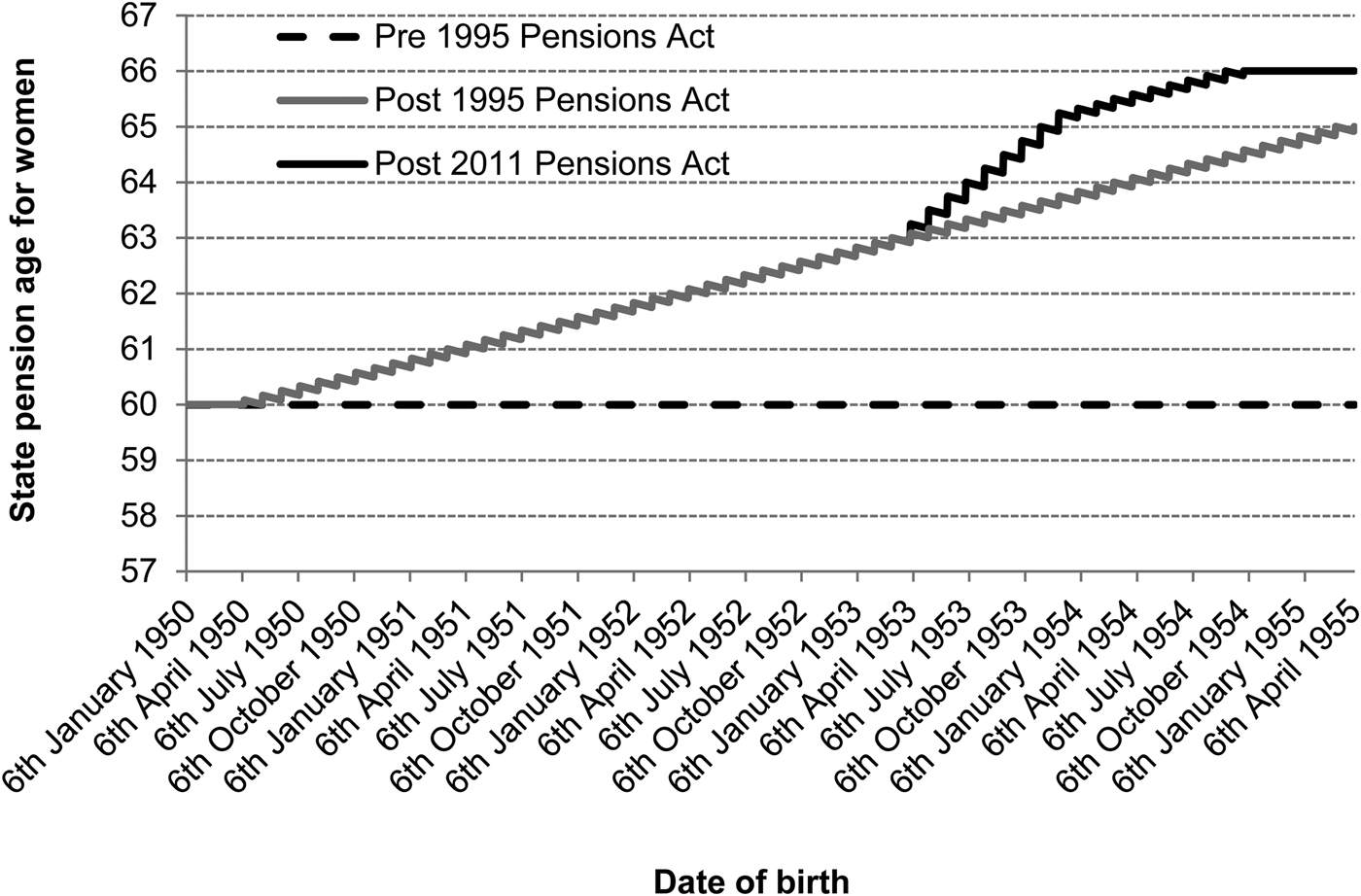
Figure 1. UK state pension age for women under different legislation. Note: The reason the state pension age increases in a ‘sawtooth’ pattern, rather than a smooth line or a ‘step’ pattern, is that women born in a given month are allocated a single ‘state pension date’ at which they are eligible for a state pension. Therefore, women born later in the month have a slightly lower state pension age than those born earlier in the month. Source: Pensions Act 1995, schedule 4 (http://www.legislation.gov.uk/ukpga/1995/26/schedule/4/enacted); Pensions Act 2007, schedule 3 (http://www.legislation.gov.uk/ukpga/2007/22/schedule/3); Pensions Act 2011, schedule 1 (http://www.legislation.gov.uk/ukpga/2011/19/schedule/1/enacted).
Household incomes are also affected by the personal tax and benefit system, some features of which become more generous when an individual reaches the state pension age. On the tax side, employee payroll taxes (National Insurance contributions) are payable on the earnings of those below the state pension age, but not on the earnings of those above the state pension age. On the benefits side, those under the state pension age who are not in paid work may be eligible for certain benefits (such as income support, jobseeker's allowance (JSA) and employment and support allowance (ESA)). When an individual (man or woman) reaches the female state pension age, they are no longer eligible for working-age benefits, but instead, if they are on a sufficiently low income, they may receive pension credit. This means-tested benefit is more generous than working-age benefits: not only is the maximum award much higher (in 2015–16, it was worth up to £151.20 ($196) per week for a single person, which is more than twice the maximum £73.10 ($95) per week paid to a single JSA recipient aged 25 or over) but it also comes with less ‘conditionality’ – no requirements for recipients to seek work or to attend work-focused interviews.
Finally, if one individual in a household is over the female state pension age then they become eligible for a winter fuel payment worth £200 ($260) per year per household (or £300 ($390) per year if at least one person is aged 80 or over).
2 Data
We used data from the UK's Family Resources Survey (FRS). This is an annual cross-sectional household survey which contains around 20,000 households per year across England, Scotland, Wales and Northern Ireland. It is available up to and including the financial year 2015–16. The survey contains a battery of questions about incomes from all sources, of all individuals in the household, alongside background information such as sex, age, education, housing tenure and household structure. Importantly, since 2008–09, it contains the exact date of birth for all individuals, which allows us to calculate their state pension age. We used the comprehensive and consistent measures of income that are derived from the FRS in order to produce the UK's official statistics on income poverty, and the distribution of income, known as the ‘Households Below Average Income’ (HBAI) statistics.Footnote 3
We also measured income poverty in the same way as the UK's official absolute poverty measure – defined as having a household net equivalised income that is below 60% of the median in 2010–11, after adjusting for household inflation.Footnote 4 Net household income is measured by summing all income from private sources (such as income from employment, private or occupational pensions, and investments), deducting direct taxes paid on this income, and finally adding all income from state transfers or benefits (including the state pension). We used measures of income poverty based on incomes both before housing costs are deducted (‘BHC’) and after housing costs are deducted (‘AHC’). When incomes are equivalised, they are equivalised using the OECD modified equivalence scale and expressed as equivalent levels of income for a couple with no dependent children (since this is the most common family type among women aged 60–62). For a childless couple in 2015–16, the (BHC) absolute poverty line is a net income of £278 ($361) per week, and for a single adult £186 ($242) per week.Footnote 5
We adjusted for inflation using a modified version of the Consumer Prices Index that also incorporates owner-occupied housing costs – the same measure of inflation as the UK's Department for Work and Pension uses when constructing their official statistics on incomes and poverty. All cash figures are expressed in 2015–16 prices. Given that there is known to be considerable measurement error in survey measures of income at the very bottom of the income distribution (Brewer et al., Reference Brewer, Etheridge and O'Dea2017) and the very top (Burkhauser et al., Reference Burkhauser, Hérault, Jenkins and Wilkins2017), in each year of the data we excluded individuals who are in households that have the lowest 1%, and the highest 1% of household incomes.
Important drivers of the effect of increasing the state pension age on women's incomes will be the extent to which state benefit incomes and income from employment respond to the reform. Figure 2a and b provide graphical evidence of the impact on these outcomes, showing how mean benefit and employment incomes have changed from 2004–05 to 2015–16, for women aged 58–63. Figure 2a shows that prior to April 2010, average incomes were much higher among those aged 60 and over than among those aged 58 or 59 (and hence below the state pension age). It shows that after April 2010/April 2012/April 2014, mean benefit incomes fell substantially (but not to zero) for women aged 60/61/62, respectively, coinciding with the times at which affected age groups could no longer receive the state pension. At the same time, Figure 2b shows that there were rises in mean employment income coinciding with women of each age no longer being eligible for the state pension, consistent with the evidence in Cribb et al. (Reference Cribb, Emmerson and Tetlow2016) that one effect of the reform is for employment income to increase to offset (at least partially) the fall in benefit income paid to households resulting from the reform.

Figure 2. (a) Mean state benefit income of women aged 58–63, 2004–05 to 2015–16. Source: Authors’ calculations using the Family Resources Survey. Number of observations: 24,493. (b) Mean gross income from employment for women aged 58–63, 2004–05 to 2015–16. Source: Authors’ calculations using the Family Resources Survey. Number of observations: 24,493.
In addition to the data on incomes, the FRS contains questions regarding families’ levels of ‘material deprivation’. These questions ask whether families are able to afford certain material items. Given that household incomes will not perfectly reflect the standard of living of a given household, we estimate whether increasing the state pension age affects the probability that families report not being able to afford certain items. This paper looks at the effect on six items that have been reported consistently since 2008–09. The FRS questions are designed explicitly to measure whether individuals are experiencing material deprivation, although it is possible that there might be effects on other indicators of deprivation/other items that are not measured in these data. The FRS survey asks whether families can afford to:
(1) keep their home in a good state of decoration;
(2) have home contents insurance;
(3) put away £10 savings per month for a rainy day;
(4) replace worn-out furniture;
(5) replace broken electrical items;
(6) have a small amount of money to spend on themselves.
These questions ask whether individuals can afford these things now. They are therefore likely to be a measure of current living conditions, rather than reflecting living standards over a longer (backward looking) period.Footnote 6 These ‘material deprivation’ questions are only asked to families if all adults are aged 64 or under; there is a separate set of ‘pensioner material deprivation’ questions for families with an adult aged 65 or over. However, from 2011 to 2012, families are only asked the material deprivation questions listed above if all adults are under the state pension age. We discuss how we estimate the impact on material deprivation in light of this in Section 4.
3 Empirical methodology
We estimate the impact of increasing the state pension age on different measures of household income, exploiting the fact that we have data on the incomes of otherwise similar women who face different state pension ages. We utilise a difference-in-differences methodology in the same way as Cribb et al. (Reference Cribb, Emmerson and Tetlow2016), who estimate the impact of the same reform on labour market behaviour using similarly structured data. This is done by estimating the following model:
 $$y_{ict} = \alpha ({\rm underSPA})_{ict} + \; \gamma _t + \lambda _c + \mathop \sum \limits_a \delta _a\left[ {{\rm ag}{\rm e}_{ict} = a} \right] + X_{ict}\beta + \varepsilon _{ict},$$
where the outcome of interest (y ict) for individual i, from cohort c, and observed in time period t is allowed to vary by whether the woman is aged below or above the state pension age (underSPA) plus a set of controls. The dummy ‘underSPA’ measures whether, at the point they are observed, they have reached their state pension age. This is constructed by comparing the date of interview in the survey, to the individuals’ state pension date (which depends on their date of birth, as shown in Figure 1). Given the nature of the reform, this is an interaction term between an individual's cohort and age.
We use 8 years of FRS data, from 2008–09 to 2015–16 (so two financial years of data prior to the state pension age starting to rise, up to the latest available data by when the female state pension age had reached 63). The coefficient on underSPA (α) can therefore be interpreted as the average effect of being under, rather than over, the state pension age, for 60–62 years old women over the period from 2010–11 to 2015–16.
Our sample includes women born from 1948–49 to 1955–56 (inclusive). This means that the difference-in-differences estimator essentially compares the outcomes of two cohorts (1948–49 and 1949–50) who are unaffected by the reform, with the following six cohorts, who are affected by the gradually increasing state pension age. The exact sample used is shown in Appendix Figure A1a, and we have a sample size of 19,086 women.Footnote 7
In Equation (1), since both age and calendar time are important determinants of private income (such as earnings and private pension income), we control for these flexibly with dummy variables for age in years and quarters (48 dummies included in the model) and time period (γ t) in years and quarters (31 dummies included in the model). We also control for the financial year of birth (which in the UK runs from April until March, λ c) (six dummies included in the model). We cannot control for cohort using fixed effects for year and quarter of birth, as that would be perfectly co-linear with the age and time fixed effects. Using (financial) year of birth dummies allows us to control flexibly for fixed differences between cohorts, without perfect co-linearity.Footnote 8
Our identifying assumption here is that any age effects on the outcomes of interest are constant across time and cohort, that any cohort effects are constant across time and age, and that any time effects are constant across cohort and age (which is the standard ‘common trends’ assumption used in difference-in-differences estimation). This seems likely to hold, and indeed, pre-reform Figure 2a and b shows very similar changes in the two of the main components of income – state benefits and employment income – for different age groups. This supports our common trends assumption. No other reforms to the pension, tax or welfare system changed in a way that affected different cohorts at different ages in the way that the increase in the state pension age has affected women.Footnote 9
We also include controls for a set of individual characteristics (X ict). These include education, relationship status, homeownership, region and – for those with a partner – partner's age and partner's education.Footnote 10
For continuous outcomes – specifically, different measures of income – we estimate Equation (1) using ordinary least squares. For dichotomous outcomes – such as whether a household is below or above the income poverty line, or different measures of deprivation – we estimate the equation using a probit model. Using the probit models, we calculate the average marginal effect of the treatmentFootnote 11 and estimate standard errors by bootstrapping with 1,000 replications. For all models, we cluster standard errors at the year-and-month of birth level as those born in a given month all have the same state pension date. If there are serially correlated shocks at the cohort-time level, then not clustering at this level would bias standard errors (Moulton, Reference Moulton1990; Donald and Lang, Reference Donald and Lang2007).
As described in Section 2, we cannot estimate the impact of increasing the female state pension age on material deprivation using the same sample as for the income measures since the relevant questions are not asked of women with a partner aged 65 or over or, since 2011–12, of those women who are over the state pension age. However, because we still observe families where the woman is aged 60 or over but also under the state pension age, we can still use a difference-in-differences methodology to estimate the impact on material deprivation. Specifically, we take women aged 57–62 who answer the material deprivation questions and contrast how material deprivation rates change among 60–62 years old between periods when they are over the state pension age and under the state pension age, with how material deprivation changes among 57–59 years old, who are under the state pension age in all years. To do this, we can simply estimate Equation (1) using the sample of women aged 57–62 who do not have a partner aged 65 or over and who answer the material deprivation questions. The exact sample used is shown in Appendix Table A1 and has a sample size of 10,947 women.
4 Results
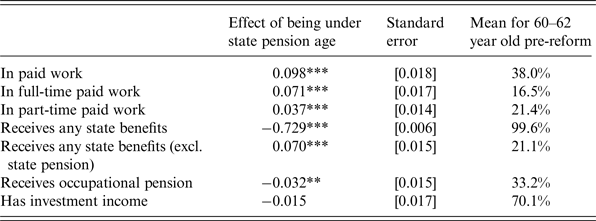
We start by looking at the impact of the state pension age on whether or not women report being in receipt of income from different sources. The estimated impacts on these dichotomous outcomes are all estimated using separate probit models, with a summary of the key results reported in Table 1. As in Cribb et al. (Reference Cribb, Emmerson and Tetlow2016), we find statistically significant evidence that being under the state pension age increases employment rates substantially, with our point estimates suggesting larger effects than they find. Our estimates suggest a 9.8 ppt increase in the proportion in paid work (from a pre-reform base of 38.0%), with a 7.1 ppt increase in full-time work and a 3.7 ppt increase in part-time work (estimated effects do not sum precisely, since they are estimated from separate models).
Table 1. Effect of increasing female state pension age from 60 to 63 on receipt of different sources of individual income (percentage points)
Note: ***, ** and * denote that the effect is significantly different from zero at the 1%, 5% and 10% levels, respectively. There are 19,086 observations in all models. All effects are obtained by estimating Equation (1) using a probit model. Standard errors are estimated by bootstrapping with 1,000 replications and are clustered at the year-and-month of birth level. The variable ‘receives any state benefits excluding state pension’ is defined as receiving any state benefit other than: the state pension, winter fuel payment and the ‘Christmas bonus’. The latter two are smaller, near-universal benefits for older individuals. Pre-reform means are estimated from FRS data from 2007–08 to 2009–10.
Unsurprisingly, being under the state pension age is found to reduce substantially the likelihood of receiving any state benefits. Pre-reform this was running at 99.6% for 60–62 years old women. Being under the state pension age is found to reduce it by 72.9 ppts. This is clearly driven by the inability to claim the state pension, as the probability of claiming a benefit other than the state pension rises by 7.0 ppts in response to the reform. This is likely to be driven by more 60–62 years old on ‘working-age’ out-of-work benefits (JSA and ESA) and potentially on in-work tax credits as more 60–62 years old women are in paid work. Looking at other sources of income, we find that being under the state pension age reduces the likelihood of receiving occupational pension income by 3.2 ppts, suggesting that a tendency to delay receipt of occupational pensions – perhaps until the state pension age or retirement – outweighs any tendency of women to draw their occupational pension income earlier in order to help make up for the loss of state pension income from the rising state pension age. We find no statistically significant effect of being under the state pension age on having investment income.
We now turn to the impact of being under the state pension age on the average (mean) level of income from different sources (with those not receiving any income from a particular source being included in the analysis as getting £0 per week). The results are reported in Table 2, with the top panel looking at individual income and the bottom panel looking at household income (i.e., taking into account income from any partner or other household members). At the time of writing, £1.00 was equivalent to approximately US$1.30 and €1.10.
Table 2. Effect of increasing female state pension age from 60 to 63 on the individual and household incomes of women (£ per week)

Note: ***, ** and * denote that the effect is significantly different from zero at the 1%, 5% and 10% levels, respectively. There are 19,086 observations in all models. All effects are obtained by estimating Equation (1) using OLS. Standard errors are clustered at the year-and-month of birth level. Pre-reform means are estimated from FRS data in 2007–08 to 2009–10.
On average, being under the state pension age is found to reduce women's individual incomes by £50 per week (compared with a pre-reform mean of £234), with an £82 per week drop in income from benefits being partially offset by a £43 per week increase in private income. The £82 per week drop in benefit income is, itself, made up of around £94 per week increase in income from the state pension, and a £12 per week rise in income from other benefits – consistent with the findings in Table 1. This increase in private income is driven by an increase in gross earnings of £44 per week (compared with a pre-reform mean of £106), with evidence (albeit only statistically significant at the 10% level) that being under the state pension age reduces occupational pension income and increases investment income by, on average, similarly small amounts.
Turning to household income, the reduction in net income is found to be smaller, at £32 per week (rather than £50 per week for individual income).Footnote 12 This is due to a bigger increase in private income (of £58 per week rather than £43 per week), partially explained by increasing the occupational pension income of the husbands of those directly affected by the reform (see Appendix Table A2). Appendix Table A2 also shows that we do not see any change in husbands’ employment rates as a result of the increase in the state pension age of their wives. In addition, we see a smaller reduction in benefit income at the household level than at the individual level (£74 per week rather than £82 per week). This could be due to a husband's entitlement to benefits increasing as a direct result of his wife being below the state pension age. This could be the case where a husband is above the female state pension age, and would therefore be entitled to an entire winter fuel payment rather than the payment being split between them, or where the husband is in receipt of means-tested benefits, such as pension credit which is reduced when his wife receives state pension income.
These results also allow us to calculate the public finance implications of raising the state pension age for women, incorporating their own behavioural changes in response to the reform and any behaviour change of their husbands that changes household incomes. By the end of 2015–16, almost 1.1 million women aged 60–62 had not yet reached state pension age. Looking at the effect of the policy on changes in benefit income, and incomes gross and net of direct taxes, implies that increasing the state pension age for women by 3 years from 60 to 63 strengthened the public finances by £5.1 billion per year (around 0.3% of GDP), of which £4.2 billion came from lower benefit payments (net of tax, where applicable) and £0.9 billion from higher direct tax payments elsewhere.
The overall reduction in benefit payments means that the reduction in spending on the state pension is only partially offset by increased spending on other benefits (such as out-of-work working-age benefits). The increase in direct tax receipts comes from the increase in employee NICs on earnings up to the (now higher) state pension age and the boost to tax receipts from behavioural responses that increase private incomes.
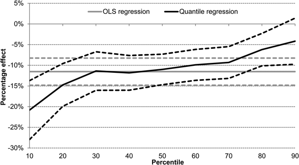
We now turn to look at the percentage change in net household income caused by being under, rather than over, the female state pension age at ages 60–62 and, in particular, we examine whether any effect varies across the income distribution. We estimate the effect of being under the state pension age on the net (equivalised) household income distribution using quantile regression. These results show how income at each percentile of the income distribution (conditional on age, cohort and the other variables that we control for as set out in Section 3) varies depending on whether an individual is under or over the state pension age. The effects are presented graphically as a percentage of household income in Figure 3 and in £ per week in Figure 4.

Figure 3. Effects of increasing female state pension age from 60 to 63 on the net equivalised household incomes of women (in percentage terms). Note: Results are obtained by estimating Equation (1) with log net equivalised household income as the dependent variable. Coefficients are converted to percentages following Halvorsen and Palmquist (Reference Halvorsen and Palmquist1980). Grey line shows the estimated mean effect from OLS, the black line from quantile regression. Quantile models are estimated using simultaneous quantile regressions, allowing for correlation in the errors across the quantiles. Standard errors for the quantile regression results are calculated by bootstrapping 1,000 times. Standard errors for OLS results are clustered at the year-and-month of birth level. The dashed lines provide the 95% confidence intervals. Number of observations: 19,086.
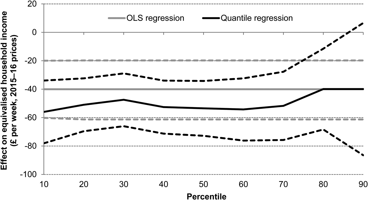
Figure 4. Effects of increasing female state pension age from 60 to 63 on the net equivalised household incomes of women (in £ per week, 2015–16 prices). Note: Results are obtained by estimating Equation (1) with net equivalised household income (expressed in 2015–16 prices) as the dependent variable. Grey line shows the estimated mean effect from OLS, the black line from quantile regression. Quantile models are estimated using simultaneous quantile regressions, allowing for correlation in the errors across the quantiles. Standard errors for the quantile regression results are calculated by bootstrapping 1,000 times. Standard errors for OLS results are clustered at the year-and-month of birth level. The dashed lines provide the 95% confidence intervals. Number of observations: 19,086.
In Figure 3, the horizontal solid grey line shows that, on average, the rise in the state pension age reduced net household incomes by 11.5% (estimated by OLS), with the horizontal dotted black lines indicating the 95% confidence interval. The solid black line shows the results from quantile regressions. This shows that the increase in the state pension age reduced incomes by a larger percentage among those towards the bottom of the income distribution than among those towards the top. Indeed, at the 90th percentile, the reduction in net household income identified is not statistically different from zero at the 5% level.
The results in Figure 4 show that this regressive pattern of losses is mainly driven by the fact that the cash reductions in income caused by the reform are similar across the income distribution. Although the point estimates are slightly smaller towards the top of the income distribution, they are not statistically different between the bottom and the top. The patterns seen in Figures 3 and 4 can be explained by the fact that state pension payments are relatively flat in cash terms across the income distribution and therefore represent a smaller share of income for those with higher private incomes.
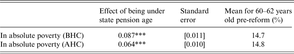
By reducing the household incomes of those towards the bottom of the income distribution, the raising of the state pension age will have pushed up recorded levels of absolute income poverty. The size of this effect can be estimated by using a probit model on whether a household is below or above the poverty line. This is done in Table 3 for two absolute income poverty lines: one measured before housing costs are deducted (BHC) and one measured after housing costs are deducted (AHC).
Table 3. Effect of increasing female state pension age from 60 to 63 on the probability of those women being in absolute income poverty (percentage points)
Note: ***, ** and * denote that the effect is significantly different from zero at the 1%, 5% and 10% levels, respectively. There are 19,086 observations in all models. All effects are obtained by estimating Equation (1) using a probit model. Standard errors are estimated by bootstrapping with 1,000 replications and are clustered at the year-and-month of birth level. Pre-reform poverty rates are estimated from FRS data in 2007–08 to 2009–10.
In both cases, we find evidence that the income poverty rate among 60–62 years old women was pushed up substantially as a result of the increase in the state pension age. For AHC poverty, our estimate suggests the poverty rate was increased by 6.4 ppts (from a pre-reform base of 14.8%), while for BHC poverty the rate was increased by 8.7 ppts (from a pre-reform base of 14.7%). Since most of the older people in the UK own their own homes outright, in order to compare their incomes with the rest of the population (who are more likely to pay rent or mortgage repayments), it is better to use an AHC measure of income.Footnote 13 We therefore put greater weight on the results for income poverty measured AHC.
In Appendix Table A3, we show that the increase in the income poverty rate caused by the increase in the state pension age varies by different characteristics. The poverty rate is consistently increased by more – in absolute terms – among those groups that had a greater pre-reform rate of poverty: singles rather than couples; renters rather than owner-occupiers; and those with no post-16 education rather than those with some post-16 education.
The analysis so far has shown that for 60–62 years old women, being below the state pension age rather than above reduces overall incomes, leads to a bigger percentage reduction in the incomes of women in lower rather than higher income households and substantially pushes up the income poverty rate. An important additional issue is whether this is a persistent effect or whether it is only temporary.
To examine whether there is evidence of any persistent effect of being under the state pension age for a longer time (which results from the increase in the state pension age) on income and poverty, we estimated Equation (1) and also added a dummy variable indicating whether the individual has not yet reached 1 year past their state pension age. The results are presented in Table 4 and show that there is some evidence that the increase in employment, and the reduction in receipt of state benefits, caused by the increase in the state pension age persist. This could suggest that some women who reach age 60 but cannot receive a state pension, and who remain in paid work as a result, then remain in paid work and do not claim their state pension when they do reach the state pension age. However, these estimates are only statistically significant at the 10% significance level.
Table 4. Testing for a persistent effect of raising state pension age: effect of increasing female state pension age from 60 to 63 on economic activity, income and poverty rate
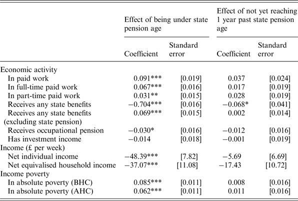
Note: ***, ** and * denote that the effect is significantly different from zero at the 1%, 5% and 10% levels, respectively. There are 19,086 observations in all models. The variable ‘receives any state benefits excluding state pension’ is defined as receiving any state benefit other than: the state pension, winter fuel payment and the ‘Christmas bonus’. All effects are obtained by estimating Equation (1) with the addition of a dummy variable signifying whether the individual has reached 1 year past her state pension age. All effects are estimated using a probit model. Standard errors are estimated by bootstrapping with 1,000 replications and are clustered at the year-and-month of birth level.
Overall, the estimated impact on net income (measured at the individual or household level) 1 year after reaching state pension age is negative, but it is much smaller than the effect on being under the state pension age, and the estimated effects are not statistically significant. In terms of the poverty rate, while this is found to increase significantly when women aged 60–62 are not able to receive the state pension, there is no evidence that this increased poverty rate persists once they do reach the state pension age. We therefore find that increasing the state pension age increases income poverty rates temporarily, rather than permanently. In other words, increasing the state pension age above 60 increases poverty rates between age 60 and the new state pension age, but has no impact on income poverty once the women have reached the higher state pension age.
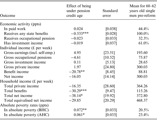
Both men and women can be eligible for pension credit and winter fuel payment when they reach the female state pension age (rather than their respective state pension ages). This means that single men are no longer able to claim pension credit at 60 (subject to the means test), but must wait until they reach the female state pension age determined by their date of birth. To examine the impact this change has on single men, we take single men from the same survey years and birth cohorts as our main analysis of women and look to see what effect the rising state pension age has on their incomes. The results are presented in Appendix Table A4 and show that the increase in the female state pension age reduces their state benefit income significantly (by £21 per week), leading to an increase in the income poverty rate among this group that is similar in magnitude to that found for women (7.2 ppts and 6.1 ppts for BHC and AHC poverty for single men, compared with 8.7 ppts and 6.4 ppts for women).
To help gauge the extent to which the reform increases hardship for the affected women, we also investigate its effect on material deprivation. Table 5 shows the impact of increasing the female state pension age on measures of material deprivation. The first four rows show that using the slightly different sample from the results shown previously makes very little difference to the estimated results of the impact of the reform on income poverty, whether it measured AHC or BHC. The table also shows that, despite the increases in income poverty as a result of the reform, there is no increase in the average number of items that families reporting being deprived of, at least using the items that we observe in our data. Nor are there any significant impacts on the probability of reporting being deprived of at least one item, or indeed any of the individual items that we examine. Not only are the effects not significantly different from zero, but the point estimates are also very close to zero. These results, which show that while there are large changes in income poverty as women become eligible for their state pension but not in material deprivation, are similar to the findings in Milligan (Reference Milligan2008) that finds sharp drops in income poverty at age 65 (when individuals can receive a means-tested pension), but no change in consumption poverty. Our results are consistent with these households being able to smooth their consumption against falls in income, and therefore avoided higher levels of deprivation despite the falls in household incomes caused by the policy.
Table 5. Effect of increasing female state pension age from 60 to 63 on material deprivation rates of women (percentage points unless otherwise stated)

Note: ***, ** and * denote that the effect is significantly different from zero at the 1%, 5% and 10% levels, respectively. There are 10,947 observations in all models. Effects on all outcomes except ‘mean number of items deprived of’ (which is estimated by OLS) are obtained by estimating Equation (1) using a probit model. Their standard errors are estimated by bootstrapping with 1,000 replications (except for ‘mean number of items deprived of’) and are clustered at the year-and-month of birth level. Pre-reform means are estimated from FRS data in 2007–08 to 2009–10.
5 Conclusion
One potential way to deal with the public finance costs of rising longevity is to increase the age at which unreduced public pensions can be received. The impact such a reform has on household incomes – and on the public finances – will depend on how households respond to the reform, and the operation of the rest of the tax and benefit system. The impact on household incomes and on the public finances will be muted if public pensions are taxable and if many individuals move onto other state benefits. If in contrast individuals respond by increasing their earnings, this would not only boost household incomes – thereby making up for at least some of the lost public pension income – but would also strengthen the public finances further. If household incomes are significantly reduced, then the gains to the public finances from such a reform should possibly be weighed against whether particular types of households experience large losses and the hardship this causes.
This paper has estimated the impact of increasing the female state pension age in the UK from 60 to 63, between April 2010 and March 2016, on the incomes of women aged 60–62. We find that, on average, household incomes were reduced by £32 per week, with an increase in employment income partially offsetting a larger fall in income from state benefits. After accounting for behavioural change, we estimate that the public finances were strengthened by £5.1 billion (0.3% of GDP), of which £4.2 billion came from reduced benefit spending (net of tax, where applicable) and £0.9 billion from increased direct tax receipts elsewhere. This implies that the reduction in benefit spending from the cut to state pension spending is only partially offset by higher benefit spending elsewhere, while on the tax side the reduction in income tax from state pension income is more than offset through increased taxes on private incomes.
Women from lower income households are found to experience a relatively greater cut to their net incomes, and the poverty rate among women aged 60–62 is found to increase by 6.4 ppts as a result of the state pension age rising from 60 to 63. The increases in poverty rates are greater among groups for whom income poverty is more prevalent: singles rather than those in couples; renters rather than owner-occupiers; and those with fewer, rather than more, years of formal education. But we find no evidence that this increase in income poverty persists once these women do reach the state pension age. We also find no evidence of any increase in the likelihood of women reporting being deprived of important material items, potentially suggesting that many affected families have smoothed their consumption, and avoided increased levels of deprivation, despite the large reduction in income caused by the reform.
Acknowledgements
The authors are grateful to the Joseph Rowntree Foundation (JRF) for funding this work. The authors are also grateful to the Economic and Social Research Council for support through the Centre for the Microeconomic Analysis of Public Policy at IFS (grant reference ES/M010147/1). The authors would like to thank James Banks, Helen Barnard, Andrew Hood and Robert Joyce, as well as members of the JRF Steering Group, participants at the Work and Pensions Economics Group Conference, and three anonymous referees, for helpful comments. Data from the Family Resources Survey were made available by the Department for Work and Pensions. Any errors and all views expressed are those of the authors.
Appendix
Table A1a. Number of observations by age and cohort for estimation sample for results on economic activity, income and poverty

Table A1b. Number of observations by age and financial year for estimation sample for material deprivation results

Table A2. Effect of increasing female state pension age from 60 to 63 on the incomes and economic activity of the husbands of affected women

Table A3. Effect of increasing female state pension age from 60 to 63 on the probability of those women being in absolute poverty (AHC) for different subgroups
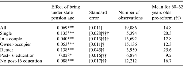
Table A4. Effect of increasing pension credit age from 60 to 63 on economic activity, incomes and poverty of single men


 Open access