


1. Introduction
Wetting presents the basic state when a finite volume of liquid contacts a solid substrate (De Gennes Reference De Gennes1985; Bonn et al. Reference Bonn, Eggers, Indekeu, Meunier and Rolley2009). The requirement for wetting differs for different applications and, hence, the design principles. For example, good wetting enables efficient liquid supply and avoids drying out in phase change thermal management, e.g. electronics cooling (Mudawar Reference Mudawar2001). In condensation, a quick wetting transition will increase the substrate's thermal resistance and worsen the condensation performance (Rose Reference Rose2002). A full understanding of the interplay between wetting and phase change is thus necessary for on-demand design of various energy systems (Wang, Zhang & Li Reference Wang, Zhang and Li2017; Breitenbach, Roisman & Tropea Reference Breitenbach, Roisman and Tropea2018; Tu et al. Reference Tu, Wang, Zhang and Wang2018) and in other microfluids-based industries (Teh et al. Reference Teh, Lin, Hung and Lee2008; Zheng et al. Reference Zheng, Bai, Huang, Tian, Nie, Zhao, Zhai and Jiang2010; Chen et al. Reference Chen, Li, Omori, Yamaguchi, Ikuta and Takahashi2022; Cheng et al. Reference Cheng, Li, Wang, Fukunaga, Teshima and Takahashi2024).
The wetting dynamics of non-volatile liquids are known to be governed by capillary force and viscous dissipation. Specifically, the spreading rate of a non-volatile Newtonian droplet in perfect wetting cases can be quantitatively described by Tanner's law,  $R(t)\sim t^{1/10}$ (Tanner Reference Tanner1979; Lelah & Marmur Reference Lelah and Marmur1981; Blake Reference Blake2006), which can be derived mathematically by employing the lubrication approximation and balancing the effect of capillary forces with the resisting viscous forces generated by the droplet motion (Voinov Reference Voinov1976; Carlson Reference Carlson2018; Pang & Náraigh Reference Pang and Náraigh2022). The spreading law has then been validated by successive experiments (Marmur Reference Marmur1983) and further extended to non-Newtonian liquids (Rafaï, Bonn & Boudaoud Reference Rafaï, Bonn and Boudaoud2004; Jalaal, Stoeber & Balmforth Reference Jalaal, Stoeber and Balmforth2021), gravity-influenced cases (Cazabat & Stuart Reference Cazabat and Stuart1986), near-critical cases (Saiseau et al. Reference Saiseau, Pedersen, Benjana, Carlson, Delabre, Salez and Delville2022), liquids on non-rigid solids and on thin liquid films (Carré, Gastel & Shanahan Reference Carré, Gastel and Shanahan1996; Cormier et al. Reference Cormier, McGraw, Salez, Raphaël and Dalnoki-Veress2012), as well as under-liquid systems (Goossens et al. Reference Goossens, Seveno, Rioboo, Vaillant, Conti and De Coninck2011; Mitra & Mitra Reference Mitra and Mitra2016).
Compared with non-volatile liquids, the spreading of volatile liquids is more complex and remains elusive owing to the complexity added by interfacial phase change and non-equilibrium thermal transport (Berteloot et al. Reference Berteloot, Pham, Daerr, Lequeux and Limat2008; Jambon-Puillet et al. Reference Jambon-Puillet, Carrier, Shahidzadeh, Brutin, Eggers and Bonn2018; Wang et al. Reference Wang, Orejon, Sefiane and Takata2019, Reference Wang, Orejon, Sefiane and Takata2020, Reference Wang, Orejon, Takata and Sefiane2022). Specifically, the non-uniform mass flux tends to recede the liquid–air interface especially near the three phase contact line. The effect of evaporation cooling and the non-uniform pathway for heat dissipation induce temperature gradient and therefore thermal Marangoni flow, which complex the flow pattern inside the droplet and further affect the spreading dynamics.
A full elucidation of these interacting mechanisms requires a quantitative description of each physical process, as well as a thorough understanding of all influencing parameters. In this research, we combine experimental and numerical approaches to address these issues and revisit the theoretical descriptions of flow interaction in liquid spreading. The explorations enable us to quantify the strength of dominating physics that varies spatially and temporally, which on the other hand provides a unifying criterion for flow reversal (Hu & Larson Reference Hu and Larson2005; Ristenpart et al. Reference Ristenpart, Kim, Domingues, Wan and Stone2007; Xu & Luo Reference Xu and Luo2007; Xu, Luo & Guo Reference Xu, Luo and Guo2010), pattern formation (Deegan et al. Reference Deegan, Bakajin, Dupont, Huber, Nagel and Witten1997; Hu & Larson Reference Hu and Larson2006; Li et al. Reference Li, Lv, Li, Quéré and Zheng2015) and Marangoni–capillary interactions (Tsoumpas et al. Reference Tsoumpas, Dehaeck, Rednikov and Colinet2015; Shiri et al. Reference Shiri, Sinha, Baumgartner and Cira2021; Yang et al. Reference Yang, Wu, Doi and Man2022) in drying droplets.
Specifically, we investigate the flow state and the resulting wetting dynamics of volatile liquids on thermal conductive substrates. In the numerical aspect, previous lubrication-type models usually consider boundary conditions with uniform heating (Anderson & Davis Reference Anderson and Davis1995; Ajaev Reference Ajaev2005) or preset substrate temperature/temperature gradient (Karapetsas, Sahu & Matar Reference Karapetsas, Sahu and Matar2013; Dai et al. Reference Dai, Khonsari, Shen, Huang and Wang2016; Charitatos & Kumar Reference Charitatos and Kumar2020; Wang et al. Reference Wang, Karapetsas, Valluri, Sefiane, Williams and Takata2021), which failed to illustrate the non-negligible role of non-isothermal heat conduction in the overall process. In addition, the numerical and experimental investigations have at large been developing in parallel without strict comparisons that consider the specific application scenarios. In this work we take account of the mass, momentum and energy transport in the liquid phase, as well as the heat conduction through the solid substrate. We apply the assumption of a precursor film (ultrathin adsorbed liquid layer; Kavehpour, Ovryn & McKinley Reference Kavehpour, Ovryn and McKinley2003; Ajaev Reference Ajaev2005; Hoang & Kavehpour Reference Hoang and Kavehpour2011) existing in front of the three-phase contact line, which eliminates the stress singularity and avoids experimental fitting of contact line motion, e.g. preset advancing/receding contact angles or a finite slip. A strict one-to-one comparison is then conducted between experimental and numerical results for a broad range of liquid–solid combinations. The reliability of the theoretical models further give rise to a general principle of flow transition and spreading rate of volatile droplets.
The rest of this paper is organised as follows. In § 2, we introduce the formulated mathematical model, the scaling and simplification and the numerical method. Section 3 introduces the material preparation, the detailed experimental set-up and procedures. Section 4 presents the numerical and experimental results including the dominating mechanisms, the transition of flow pattern and their relations to the spreading dynamics. Section 5 summarises the key findings of this work, and shares our perspectives on liquid spreading with/without interfacial phase change.
2. Formulation of the numerical model
We consider a thin liquid droplet (Newtonian fluid, with aspect ratio  $\varepsilon = \hat {H}_0/\hat {R}_0\ll 1$, where $\hat {H}_0$ is the initial droplet height, $\hat {R}_0$ is the initial droplet contact radius) sitting on a thermal conductive solid substrate with finite thickness and surrounded by a mixture of its own vapour and non-condensing gas, e.g. a water droplet in humid air, as indicated by figure 1(a). The low aspect ratio allows for the application of lubrication theory which simplifies the Navier–Stokes equations, while capturing the dominating physical processes. The lubrication approximation is valid for droplets with small and moderate contact angles typically less than $40^{\circ }$, which is the case of current research on complete wetting and partial wetting scenarios. A precursor film is assumed to exist at the solid surface in front of the three phase contact line. This avoids the stress singularity that may arise due to the inherent contradiction in simultaneously assuming the no-slip boundary condition and expecting a displacement between liquid and solid with contact line motion.

Figure 1. (a) A single component droplet with small aspect ratio,  $\hat {H}_0/\hat {R}_0$, sitting on a solid substrate surrounded by its own vapour and non-condensing gas. Here $c_{sat}$ denotes the saturation vapour concentration. We use $\hat T_{g}$ and $c_{g}$ to denote the temperature and vapour concentration of the gas phase, which remain constant. Here $\hat {\rho }$ is the liquid density, $\hat {\mu }$ is the liquid viscosity, $\hat {k}$ is the thermal conductivity of the liquid, $\hat {c_p}$ is the specific heat capacity of the liquid, $\hat {H}_{solid}$ is the thickness of the substrate, $\hat {k}_{solid}$ is the thermal conductivity of the substrate, $T_{w}$ is the temperature at the downward side of the substrate and $\vec n$ and $\vec t$ are the outward units vectors acting in normal and tangential directions to the interface. The centre of droplet base, O, is defined as the origin of the coordinate. (b) Governing equations that are considered in the gas, liquid and solid phases, along with the boundary equations at the central axis, the liquid–gas interface and the liquid–solid interface.
2.1. Governing equations
A cylindrical coordinate system,  $(\hat {r},\theta,\hat {z})$, is applied to solve the velocity field, $\hat {\boldsymbol {u}}=(\hat {u},\hat {v},\hat {w})$, where $\hat {u}$, $\hat {v}$ and $\hat {w}$ correspond to the horizontal, azimuthal and vertical components of the velocity field, respectively. The liquid–vapour interface locates at $\hat {z}=\hat {h}(\hat {r},\hat {t})$ and the liquid–solid at $\hat {z}=0$. The liquid phase is governed by the continuity, momentum and energy equations (figure 1(b)),
 \begin{gather} \hat{\boldsymbol{\nabla}}\boldsymbol{\cdot} \hat{\boldsymbol{u}} = 0, \end{gather}
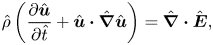 \begin{gather} \hat{\rho}\left(\frac{\partial\hat{\boldsymbol{u}}}{\partial\hat{t}}+\hat{\boldsymbol{u}}\boldsymbol{\cdot} \hat{\boldsymbol{\nabla}} \hat{\boldsymbol{u}}\right)=\hat{\boldsymbol{\nabla}} \boldsymbol{\cdot} \hat{\boldsymbol{E}}, \end{gather}
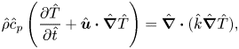 \begin{gather} \hat{\rho}\hat{c}_p\left(\frac{\partial\hat{T}}{\partial\hat{t}}+\hat{\boldsymbol{u}}\boldsymbol{\cdot} \hat{\boldsymbol{\nabla}} \hat{T}\right)=\hat{\boldsymbol{\nabla}} \boldsymbol{\cdot} (\hat{k}\hat{\boldsymbol{\nabla}}\hat{T}), \end{gather}
where liquid density  $\hat {\rho }$, specific heat capacity $\hat {c}_p$ and thermal conductivity $\hat {k}$ are set as constant, $\hat {T}$ denotes temperature, $\hat {t}$ denotes time and $\hat {\boldsymbol {E}}$ denotes the total stress tensor at the liquid side,
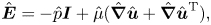 \begin{equation} \hat{\boldsymbol{E}}={-}\hat{p}\boldsymbol{I}+\hat{\mu}(\hat{\boldsymbol{\nabla}}\hat{\boldsymbol{u}}+\hat{\boldsymbol{\nabla}}\hat{\boldsymbol{u}}^{\rm T}), \end{equation}
where  $\hat {p}$ is the pressure of the liquid phase, $\hat {\mu }$ is the dynamic viscosity of the liquid and is set as constant and $\boldsymbol {I}$ is the identity tensor.
At the liquid–gas interface, the liquid velocity and geometry satisfy a force balance both in the normal and tangential directions (figure 1(b)). The normal stress balance relates the pressure difference, surface tension, mean curvature and van der Waals interactions,
 \begin{equation} -\hat{p}+\boldsymbol{n}\boldsymbol{\cdot} \hat{\boldsymbol{\tau}}\boldsymbol{\cdot} \boldsymbol{n}=2\hat{\kappa}\hat{\sigma}+\hat{\varPi}-\hat{p}_g, \end{equation}
where  $\hat {p}_g$ is the total pressure of the gas phase, $\hat {\sigma }$ is the liquid–gas surface tension, $\hat {\boldsymbol {\tau }}$ is the extra stress tensor of the liquid phase. $2\hat {\kappa }=-\hat {\boldsymbol {\nabla }}_S\boldsymbol {\cdot }\boldsymbol {n}$ is twice the mean curvature of the free surface, $\hat {\boldsymbol {\nabla }}_S=(\boldsymbol {I}-\boldsymbol {n}\boldsymbol {n})\boldsymbol {\cdot }\hat {\boldsymbol {\nabla }}$ is the surface gradient operator. Here $\hat {\varPi }$ denotes the disjoining pressure between interfaces that accounts for intermolecular interactions (De Gennes, Hua & Levinson Reference De Gennes, Hua and Levinson1990),
 \begin{equation} \hat{\varPi}=\frac{\hat{A}}{6{\rm \pi}\hat{h}^3}, \end{equation}
with  $\hat {A}$ being the dimensional Hamaker constant, $\hat {h}$ being the location of the liquid–gas interface.
The tangential stress balance relates the shear stress and the surface tension gradient. By ignoring the shear stress from the gas phase due to small viscosity, we arrive at
 \begin{equation} \boldsymbol{n}\boldsymbol{\cdot}\hat{\boldsymbol{E}}\boldsymbol{\cdot}\boldsymbol{t} =\hat{\boldsymbol{\nabla}}_S\hat{\sigma}\boldsymbol{\cdot}\boldsymbol{t}, \end{equation}
where  $\boldsymbol {t}$ refers to the outward vector which is tangential to the interface.
The motion of the liquid–gas interface (free surface) can be described with the kinematic boundary condition, expressed as
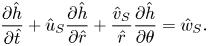 \begin{equation} \frac{\partial\hat{h}}{\partial\hat{t}}+\hat{u}_S\frac{\partial\hat{h}}{\partial\hat{r}}+\frac{\hat{v}_S}{\hat{r}} \frac{\partial\hat{h}}{\partial\theta}=\hat{w}_S. \end{equation}
 The boundary equation of mass balance (liquid–gas) can be expressed by the relationship between the velocity of the liquid solution,  $\boldsymbol {\hat {u}}$, the velocity of the liquid–gas interface, $\boldsymbol {\hat {u}}_S=(\hat {u}_S,\hat {v}_S,\hat {w}_S)$, and the interfacial mass flux, $\hat {J}$:
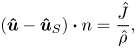 \begin{equation} (\boldsymbol{\hat{u}}-\boldsymbol{\hat{u}}_S)\boldsymbol{\cdot} n=\frac{\hat{J}}{\hat{\rho}}, \end{equation}
where  $\hat {J}$ denotes the interfacial mass flux of evaporating liquid. The jump energy balance can then be derived accounting for the heat release at the liquid–vapour interface and ignoring the heat conduction into the gas phase. This assumption is reasonable in cases where $\hat {k}_{air}\ll \hat {k}$:
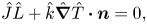 \begin{equation} \hat{J}\hat{L}+\hat{k}\hat{\boldsymbol{\nabla}}\hat{T}\boldsymbol{\cdot}\boldsymbol{n}=0, \end{equation}
where  $\hat {L}$ denotes the latent heat of vapourisation.
The Hertz–Knudsen equation is commonly used for predicting the mass flux induced by evaporation or condensation towards a liquid–vapour interface. The following relation can be derived combining the Hertz–Knudsen equation (Plesset & Prosperetti Reference Plesset and Prosperetti1976; Moosman & Homsy Reference Moosman and Homsy1980), the chemical potential difference across the liquid–gas interface (Atkins, Atkins & de Paula Reference Atkins, Atkins and de Paula2014), and the ideal gas assumption,
 \begin{equation} \hat{J}=\hat{p}_{v,sat}\sqrt{\frac{\hat{M}}{2{\rm \pi}\hat{R}_g\hat{T}_g}}\left(\frac{\hat{M}}{\hat{\rho}\hat{R}_g\hat{T}_g} (\hat{p}-\hat{p}_g)+\frac{\hat{M}\hat{L}}{\hat{R}_g\hat{T}_g^2}(\hat{T}_S-\hat{T}_g)+\ln\left(\frac{1}{\chi_{vapour}}\right)\right), \end{equation}
where  $\hat {p}_{v,sat}$ is the saturation vapour pressure, $\hat {M}$ is the molar mass of the liquid, $\hat {R}_g$ is the gas constant, $\hat {T}_g$ is the temperature of gas phase, $\hat {T}_S$ is the temperature at the liquid–gas interface and $\chi _{vapour}$ is the relative vapour concentration, i.e. ratio of partial vapour pressure to saturation vapour pressure in the gas phase.
2.2. Scaling
The key parameters are scaled as follows:
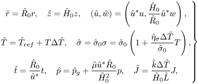 \begin{equation} \left. \begin{gathered} \hat{r}=\hat{R}_0 r,\quad \hat{z}=\hat{H}_0 z,\quad (\hat{u},\hat{w})=\left(\hat{u}^*u,\frac{\hat{H}_0}{\hat{R}_0}\hat{u}^*w\right),\\ \hat{T}=\hat{T}_{ref}+T\Delta \hat{T}, \quad \hat{\sigma}=\hat{\sigma}_0\sigma=\hat{\sigma}_0\left(1+\frac{\hat{\eta}_\sigma \Delta\hat{T}}{\hat{\sigma}_0}T\right),\\ \hat{t}=\frac{\hat{R}_0}{\hat{u}^*}t,\quad \hat{p}=\hat{p}_g+\frac{\hat{\mu}\hat{u}^*\hat{R}_0}{\hat{H}_0^2}p,\quad \hat{J}=\frac{\hat{k}\Delta\hat{T}}{\hat{H}_0\hat{L}}J, \end{gathered} \right\} \end{equation}
where the characteristic velocity is defined as  $\hat {u}^*={\varepsilon \hat {\eta }_\sigma \Delta \hat {T}}/{\hat {\mu }}$, $\hat {\sigma }_0$ is the liquid–gas surface tension at reference temperature, $\hat {\eta }_\sigma$ is the coefficient of surface tension to temperature, $\hat {T}_{ref}$ is the reference temperature and $\Delta \hat {T}$ is the maximum temperature difference across the droplet. The dimensionless group is thereafter derived, including the Reynolds number ${Re}={\hat {\rho }\hat {u}^*\hat {H}_0}/{\hat {\mu }}$ (ratio of inertia to viscous effect), Prandtl number ${Pr}={\hat {\mu }\hat {c}_{p}}/{\hat {k}}$ (ratio of momentum diffusivity to thermal diffusivity), evaporation number $E={\hat {k}\hat {R}_0\Delta \hat {T}}/{\hat {\rho }\hat {L}\hat {H}_0^2\hat {u}^*}$ (measure of evaporation strength), Marangoni number ${Ma}={\hat {\mu }\hat {u}^*}/{\varepsilon \hat {\sigma }_0}={\hat {\eta }_\sigma \Delta \hat {T}}/{\hat {\sigma }_0}$ (measure of the strength of Marangoni flow), Hamaker constant $\mathcal {A}={\hat {\mathcal {A}}}/{6{\rm \pi} \hat {\mu }\hat {u}^*\hat {R}_0\hat {H}_0}$, the coefficients in the expression of mass flux $\delta ={\hat {M}\hat {\eta }_\sigma \Delta \hat {T}}/{\hat {\rho }\hat {R}_g\hat {T}_g\hat {H}_0}$ (measure of Kelvin effect), $\psi ={\hat {M}\hat {L}\Delta \hat {T}}/{\hat {R}_g\hat {T}_g^2}$ (effect of local temperature difference on the mass flux) and Jakob number ${Ja}=({\hat {k}\Delta \hat {T}}/{\hat {H}_0\hat {L}\hat {p}_{v,sat}})\sqrt {{2{\rm \pi} \hat {R}_g\hat {T}_g}/{\hat {M}}}$ (measuring the joint thermal effects at the interface by evaporation cooling and heat dissipation into the liquid).
For sessile droplets with slow interfacial phase change, the inertia effect can be neglected with very small Reynolds number (usually  $Re <10^{-1}$ for droplet wetting and evaporation), therefore we set the Reynolds number to zero in the formulation. By further ignoring the parameter variation in the azimuthal direction, we arrive at the dimensionless governing equations, including mass conservation (2.13), momentum equation (2.14), energy equation (2.15), as well as the dimensionless boundary equations, including the normal and tangential stress boundary balance (2.16), the kinematic boundary condition (2.17), the jump energy balance (2.18) and the expression of interfacial mass flux (2.19) (figure 1(b)):
 \begin{gather} \frac{1}{r}\frac{\partial(ru)}{\partial r}+\frac{\partial w}{\partial z}=0, \end{gather}
 \begin{gather} \frac{\partial p}{\partial r}=\frac{\partial}{\partial z}\left(\frac{\partial u}{\partial z}\right), \end{gather}
 \begin{gather} \frac{\partial}{\partial z}\left(\frac{\partial T}{\partial z}\right)=0, \end{gather}
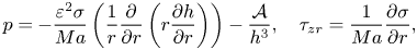 \begin{gather} p={-}\frac{\varepsilon^2\sigma}{Ma}\left(\frac{1}{r}\frac{\partial}{\partial r}\left(r\frac{\partial h}{\partial r}\right)\right)-\frac{\mathcal{A}}{h^3},\quad \tau_{zr}=\frac{1}{Ma}\frac{\partial\sigma}{\partial r}, \end{gather}
 \begin{gather} \frac{\partial h}{\partial t}+u\frac{\partial h}{\partial r}-w+EJ=0, \end{gather}
 \begin{gather} J+\frac{\partial T}{\partial z}=0, \end{gather}
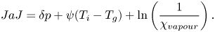 \begin{gather} {Ja}J=\delta p+\psi (T_i-T_g)+\ln\left(\frac{1}{\chi_{vapour}}\right). \end{gather}
 The above equations are integrated over the vertical direction, with the integration of velocity and temperature expressed as  $f=\int _0^h u\,\textrm {d}z$, $\varTheta =\int _0^h T\,\textrm {d}z$. The integral form of equations are subsequently discretised using a finite-element/Galerkin method; the variables are approximated using quadratic Lagrangian basis functions $\varPhi _i$. After applying the divergence theorem, we arrive at the weak form of five governing equations with five independent variables, $h$,
$h$,  $p$,
$p$,  $f$,
$f$,  $\varTheta$ and $J$:
$J$:
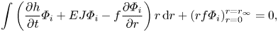 \begin{gather} \int\left(\frac{\partial h}{\partial t}\varPhi_i+EJ\varPhi_i-f\frac{\partial\varPhi_i}{\partial r}\right)r\,{\rm d}r+(rf\varPhi_i)_{r=0}^{r=r_\infty}=0, \end{gather}
 \begin{gather} \int\left(h\frac{\partial p}{\partial r}-\left(\frac{\partial u}{\partial z}\right)_0^h\right)\varPhi_i r\,{\rm d}r=0, \end{gather}
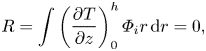 \begin{gather} R=\int\left(\frac{\partial T}{\partial z}\right)_0^h\varPhi_i r\,{\rm d}r=0, \end{gather}
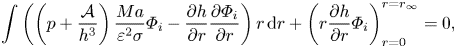 \begin{gather} \int\left(\left(p+\frac{\mathcal{A}}{h^3}\right)\frac{Ma}{\varepsilon^2\sigma}\varPhi_i-\frac{\partial h}{\partial r}\frac{\partial \varPhi_i}{\partial r}\right)r\,{\rm d}r+\left(r\frac{\partial h}{\partial r}\varPhi_i\right)_{r=0}^{r=r_\infty}=0, \end{gather}
 \begin{gather} \int\left({Ja}J-\delta p-\psi(T|_{z=h}-T_g)+\ln\chi_{vapour}\right)\varPhi_i r\,{\rm d}r=0. \end{gather}
 Finally, we consider an Ansatz distribution function of liquid temperature T and velocity u in z axis to complete the mathematical formulation. We fit the flow velocity and the temperature distribution with a parabolic expression, i.e.  $y=c_3+c_2z+c_1 z^2$, then derive their expressions by applying the boundary conditions at $z = 0$ and $z = h$.
At the liquid–gas interface,  $z = h$, the flow velocity meets the tangential stress balance (2.16), which relates the surface tension gradient to the shear stress (multiplication of dynamic viscosity and velocity gradient). At the liquid–solid interface, $z = 0$, a no slip boundary condition applies. The flow velocity is thereafter derived as
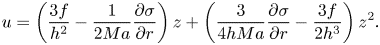 \begin{equation} u=\left(\frac{3f}{h^2}-\frac{1}{2{Ma}}\frac{\partial\sigma}{\partial r}\right)z+\left(\frac{3}{4h {Ma}}\frac{\partial\sigma}{\partial r}-\frac{3f}{2h^3}\right)z^2. \end{equation}
 For the temperature distribution, the temperature meets the jump energy balance at the droplet surface,  $z = h$, (2.18), which relates the temperature gradient at the liquid side to the interfacial heat flux due to phase change. At the liquid–solid interface, we consider (1) substrates with constant temperature and (2) thermal conductive substrates with finite thickness. For case (1) with constant substrate temperature, the temperature distribution in the liquid phase can be derived as
 \begin{equation} T=T_W+\left(\frac{3\varTheta}{h^2}-\frac{3T_W}{h}+\frac{J}{2}\right)z+\left(\frac{3T_W}{2h^2}-\frac{3\varTheta}{2h^3}-\frac{3J}{4h}\right)z^2. \end{equation}
 For case (2) thermal conductive substrates with finite thickness  $\hat {H}_{solid}$ and thermal conductivity $\hat {k}_{solid}$, the process can be simplified into a quasi-steady one-dimensional problem. Similar approximations were also adopted in research by Ristenpart et al. (Reference Ristenpart, Kim, Domingues, Wan and Stone2007), Xu et al. (Reference Xu, Luo and Guo2010) and Dunn et al. (Reference Dunn, Wilson, Duffy, David and Sefiane2009). The boundary condition at $z = 0$ in this situation can be described as:
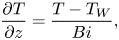 \begin{equation} \frac{\partial T}{\partial z}=\frac{T-T_W}{Bi}, \end{equation}
where Biot number,  ${Bi}=\hat {H}_{{solid}}\hat {k}/\hat {H}_0\hat {k}_{solid}$, denotes the ratio of thermal resistance of the solid phase to that of the liquid phase.
Combining the parabolic expression of temperature distribution and the boundary conditions at the liquid–solid interface and the liquid–gas interface, the distribution of liquid temperature in case (2) is thereafter derived as
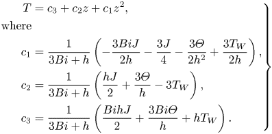 \begin{equation} \left. \begin{aligned} T & =c_3+c_2z+c_1z^2,\\ \mathrm{where} & \\ c_1 & =\frac{1}{3{Bi}+h}\left(-\frac{3{Bi}J}{2h}-\frac{3J}{4}-\frac{3\varTheta}{2h^2}+\frac{3T_W}{2h}\right), \\ c_2 & =\frac{1}{3{Bi}+h}\left(\frac{hJ}{2}+\frac{3\varTheta}{h}-3T_W\right),\\ c_3 & =\frac{1}{3{Bi}+h}\left(\frac{{Bi}hJ}{2}+\frac{3{Bi}\varTheta}{h}+hT_W\right). \end{aligned} \right\} \end{equation}
2.3. Initial and boundary conditions
In the region of  $0\leq r\leq 1$, the initial conditions, $t=0$, are set as
 \begin{equation} h(r,0)=h_\infty+1-r^2,\quad f(r,0)=0,\quad \varTheta(r,0)=h(r,0)T_W, \end{equation}
where  $h_\infty$ is the thickness of the precursor film and $T_W$ is the initial temperature of the solid substrate. For zero mass flux at the precursor film region, the initial value of $h_\infty$ is set as $\sqrt [3]{{\mathcal {A}\delta }/({\psi (T_W-T_g)-\ln (\chi _{vapour})})}$ by combining (2.19) ( $J = 0$) and (2.16), where the disjoining pressure from intermolecular interaction prevents further evaporation of the liquid film. The parameters at the droplet centre, $r = 0$, satisfy the symmetric boundary conditions, expressed as
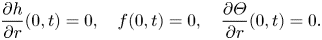 \begin{equation} \frac{\partial h}{\partial r}(0,t)=0,\quad f(0,t)=0,\quad \frac{\partial\varTheta}{\partial r}(0,t)=0. \end{equation}
 In the region of precursor film,  $r > 1$, the parameters are set as
 \begin{equation} h(r,0)=h_\infty,\quad f(r,0)=0,\quad \varTheta(r,0)=h_\infty T_W. \end{equation}
 We apply Galerkin finite-element method to solve the system of partial differential equations (PDEs). A one-dimensional mesh is constructed along the r-direction, and the length of the computational domain is set as twice the maximal spreading radius within the computational time to ensure the free development of the droplet morphology. The domain is discretised along r from 0 to  $r_\infty$ into equally spaced nodes, the total number being $N_{tot}$, and the density is set as 200 per dimensionless length with grid independence test of the solution. At each time step, we apply the Newton–Raphson method to obtain the solution across the computational domain progressively. The solution evolves forwards with an adaptive time interval which adjusts according to the maximum residual errors of the governing equations from the previous time step (adaptive implicit Euler method). The iterative program is written in Fortran, making use of the linear algebra package LAPACK.
3. Experimental method
As shown in figure 2, experiments are conducted with high-speed imaging and microPIV in an air-conditioned lab space with constant temperature and humidity ( $20\,^{\circ }\textrm {C}$, $50\pm 5\,\%$RH). We use high-speed camera (Photron FASTCAM Mini AX200 type with frame rate of 3000 fps) to trace the fast spreading of droplet upon its contact with a solid surface. To minimise the impinging force of the droplet, we set the distance between the syringe and the substrate to a similar value with the initial diameter of the spherical droplet ( $V_0 =3\pm 0.2\ \mathrm {\mu }\textrm {l}$ for 1-butanol and 2-propanol, and $0.6\pm 0.05\ \mathrm {\mu }\textrm {l}$ for FC-72), so that the droplet can touch the solid surface right after its generation from the syringe tip. A commercial cool plate based on Peltier module and digital PID controller ( $0\unicode{x2013} 105\,^\circ \textrm {C}$, ${\pm }0.2\,^\circ \textrm {C}$) is utilised as the substrate holder which keeps the downward side substrate temperature constant.

Figure 2. Experimental set-up for (a) droplet spreading and (b) microPIV visualisation of flow field inside the droplet.
We select 1-butanol, 2-propanol (IPA) and FC-72 as the working fluids, each with one order of magnitude larger saturation vapour pressure (table 1). Three types of solid materials are utilised, i.e. copper, SUS430 and glass, each with one order of magnitude smaller thermal conductivity. We also use copper substrates of thickness 0.3, 1.0 and 3.0 mm to demonstrate the effect of substrate thickness. The three types of substrates exhibit a highly wetting state for 1-butanol, 2-propanol and FC-72 which matches the requirement of low contact angle (less than  $40^{\circ }$) for lubrication approximation. For each condition, we repeated the experiments at least five times. The average values of the spreading rates along with standard deviations are derived for comparison with the numerical predictions (table 4). The key thermophysical properties of different liquids and solids are given in tables 1 and 2.
Table 1. Thermophysical properties of representative liquids at 293 K except FC-72 (298 K). 1-butanol, 2-propanol and FC-72 were utilised in present experiments. Water, 2-propanol, methanol, ethanol and chloroform were utilised in previous studies on circulation reversal (Ristenpart et al. Reference Ristenpart, Kim, Domingues, Wan and Stone2007; Xu et al. Reference Xu, Luo and Guo2010; Li et al. Reference Li, Lv, Li, Quéré and Zheng2015) as marked in figure 5. Alkanes (e.g. heptane and hexane) were utilised in the study of Shiri et al. (Reference Shiri, Sinha, Baumgartner and Cira2021) on the influence of thermal Marangoni flow on droplet geometry as marked in figure 7.
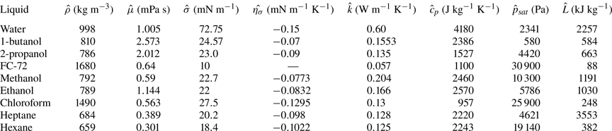
Table 2. Thermal conductivity of representative substrate materials. Copper, SUS430 and glass were utilised in present study. Glass was utilised in the work of Xu et al. (Reference Xu, Luo and Guo2010) and Hu & Larson (Reference Hu and Larson2006). Polydimethylsiloxane (PDMS) was utilised in the work of Ristenpart et al. (Reference Ristenpart, Kim, Domingues, Wan and Stone2007).
To remove any oxide residuals and ensure the uniformity and smoothness of the solid surface, we fabricate substrate surfaces with mirror finishing. The surface roughness of glass, SUS430 and copper is characterised to be  ${Sa}_{glass} = 0.258\ \mathrm {\mu }\textrm {m}$, ${Sa}_{SUS430} = 0.134\ \mathrm {\mu }\textrm {m}$, ${Sa}_{copper} = 0.291\ \mathrm {\mu }\textrm {m}$ with a 3-D laser scanning microscope (OLYMPUS/LEXT OLS4000). Before each set of experiments, we prepare the solid substrate by 15 min ultrasonic bath with 99.8 % ethanol, then flush with large quantity of deionised water, and dry the surface with high-speed clean air flow. We start the high-speed camera immediately before the deposition of the droplet and stop recording as the droplet fully spreads.
For enhancing the image contrast, an LED light sheet panel is utilised for making clear droplet shadow. The videos are further processed with imageJ (Schneider, Rasband & Eliceiri Reference Schneider, Rasband and Eliceiri2012) and Matlab for extracting the evolution of contact radius and linearly fitting the log–log plot. To avoid the inertia effect of the depositing droplet (Ding & Spelt Reference Ding and Spelt2007; Bird, Mandre & Stone Reference Bird, Mandre and Stone2008; Chen, Bonaccurso & Shanahan Reference Chen, Bonaccurso and Shanahan2013), the plot fitting focuses on inertia-free flow state regime after the droplet fully detaches from the syringe with continuous contact line advancing.
Microparticle image velocimetry ( $\mathrm {\mu }$PIV) is implemented to measure the flow field near the bottom of an evaporating droplet (figure 2b). The measurements are based on an inverted fluorescent microscope (Nikon Ts2-FL). Specifically, a green laser (468 nm) is utilised to excite the fluorescent microtracers (Fluoro-Max; green fluorescent polymer microspheres: excitation/emission 468/508 nm, diameter $1.0\ \mathrm {\mu }\textrm {m}$). A CCD camera (STC-MCS510U3V) connected to the microlens captures the fluorescent signal emitted by the tracer particles. We use butanol and IPA as the test fluids, which have similar surface tension but different volatility (table 1). Experiments are conducted on slide glass for microscope with thickness of $1.1 \pm 0.2$ mm. The droplet size for microPIV experiments is set as $0.5 \pm 0.002\ \mathrm {\mu }\textrm {l}$, and is focused with 20 $\times$ lens from the bottom. Each set of experiments is repeated for more than five times. The representative videos are presented in Supplementary movie 3 available at https://doi.org/10.1017/jfm.2024.385, where the video of butanol is speeded up by 20 times and the video of IPA is slowed down by 3 times with ImageJ.
4. Results and discussion
4.1. Transition of flow states: physical mechanisms
Figure 3 shows the evolution of flow field in a representative case, which can be characterised into three stages. At the initial stage ( ${\unicode{x2460}}$) when a liquid droplet contacts a solid surface, the capillary effect drives a continuous outward flow, leading to rapid droplet spreading. In the second stage ( ${\unicode{x2461}}$), the evaporation cooling effect and the non-uniform heat dissipation result in temperature gradient across the droplet surface, and induce thermal Marangoni flow from the droplet edge towards the apex. The opposing thermal Marangoni and capillary forces lead to the formation of two stagnation points (SPs) at the droplet surface. The upper SP moves towards the droplet apex as the Marangoni flow gets stronger and disappears as a recirculation vortex engulfs the whole droplet. The lower SP remains near the contact line ( ${\unicode{x2462}}$) as a result of capillary–Marangoni interaction (Ristenpart et al. Reference Ristenpart, Kim, Domingues, Wan and Stone2007; Xu & Luo Reference Xu and Luo2007; Wang & Harris Reference Wang and Harris2018; Wang et al. Reference Wang, Karapetsas, Valluri and Inoue2024).
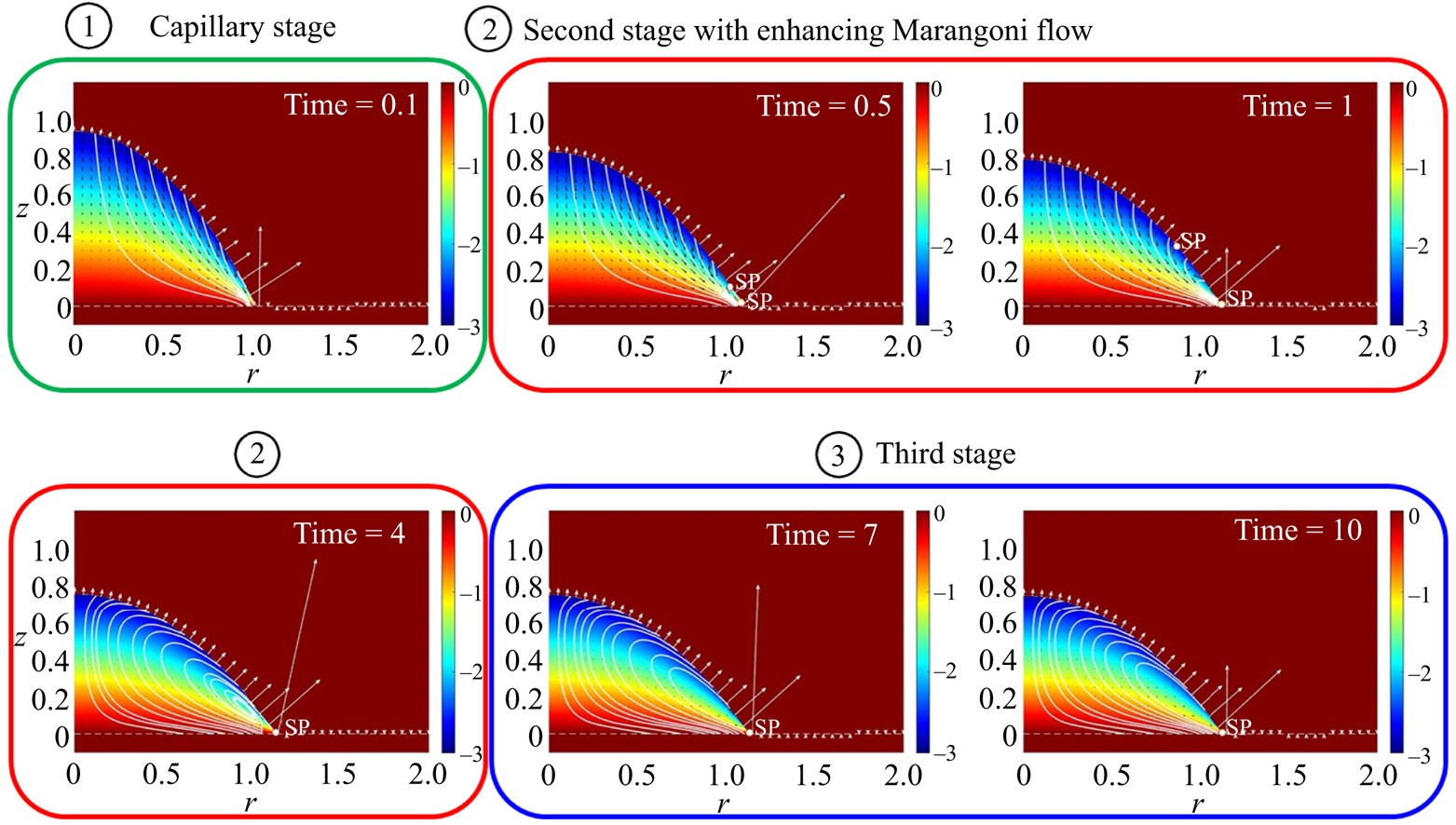
Figure 3. Evolution of flow state for an evaporative droplet on a thermal conductive substrate. The three stages are classified according to the state of internal flow, where continuous outwards capillary flow dominates droplet spreading at the initial stage, the Marangoni flow develops at the second stage and balances with the capillary flow at the third stage. The key dimensionless numbers in this case are set as  $Ja^* = 5\times 10^{-3}$, $Bi = 10^{-4}$ and $Ma = 10^{-2}$.
Yet two questions arise as our analysis goes on. One is ‘Does the SP universally exist?’ and another is ‘Does thermal Marangoni flow always play a role in wetting dynamics?’. These two questions are intricately related as the relative strength of thermal Marangoni flow and capillary flow decides the flow state and the formation of the SP, and therefore the wetting dynamics.
To elucidate this, we conducted detailed parametric analyses on varying combinations of liquids and solids that span five orders of magnitudes in their saturation vapour pressure and thermal conductivity. Two dominant dimensionless numbers (derived in the scaling process) are concluded to govern the interacting physics, namely, the Jakob number,  $Ja$, which evaluates the balance between interfacial phase change and heat transfer into the liquid phase, and the liquid–solid Biot number, $Bi$, which indicates the ratio of liquid phase to solid phase thermal resistance.
With decreasing  $Bi$, heat dissipation into the substrate becomes efficient. In such cases, thermal resistance in the liquid phase dominates, thus the temperature gradient across the droplet surface is large from the droplet apex to the edge (large difference in thermal resistance across the liquid). The large temperature gradient strengthens the Marangoni flow and retards droplet spreading.
The Jakob number, mostly related to liquid volatility, decides the strength of evaporation cooling. For moderately volatile liquids, the evaporation mass flux takes heat away from the droplet surface, while the heat supply from the substrate is also considerable. Near the contact line, the liquid film is thin, enabling good heat supply and, thus, a higher temperature in comparison to the droplet apex; this is the case for many volatile liquids such as water and alcohol. At very high liquid volatility (small  $Ja$, e.g. flash evaporation), heat supply from the substrate can no longer meet the heat loss from the droplet surface, as a result, the droplet surface gets ‘uniformly cold’, leading to weak thermal Marangoni flow. For liquids that hardly evaporate (low volatility and large $Ja$), the effect of evaporation cooling is negligible, and the process is near isothermal, which also leads to weak Marangoni effect.
Taking an overview of the dominating mechanisms, we can see that  $Ja$ (interfacial thermal effect) and $Bi$ (heat conduction into the substrate) determine the temperature field in the droplet–solid system. Once the temperature gradient establishes, the Marangoni number, $Ma={\hat {\mu }_0 \hat {{u}}^*}/{\varepsilon \hat {\sigma }_0}={\hat {\eta }_\sigma \Delta \hat {{T}}}/{\hat {\sigma }_0}$, determines the strength of the Marangoni flow. The Marangoni flow interacts with the capillary flow, which together affect the flow field inside the droplet, and further determine the droplet dynamics along with the nonuniform distribution of evaporation mass flux, as indicated by figure 4.
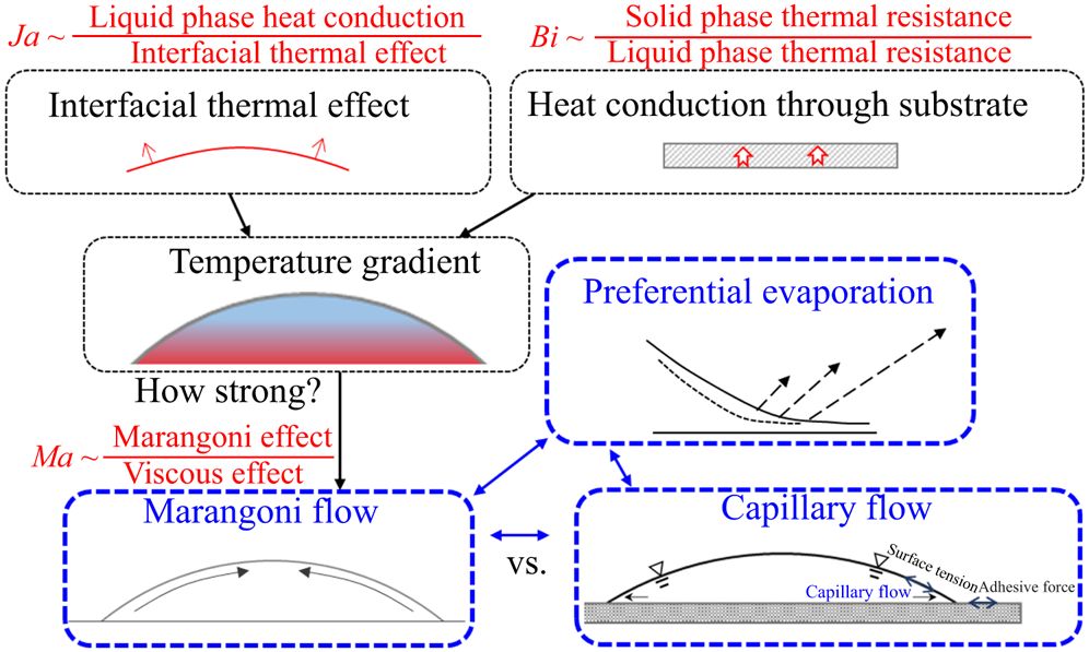
Figure 4. Decomposition of the dominating mechanisms in wetting dynamics of evaporative droplets.
4.2. Limitations of the Hertz–Knudsen equation: appropriate scaling for comparison with experiments
In the mathematical model, we formulate the expression of interfacial mass flux by combining the Hertz–Knudsen equation, the chemical potential difference across the liquid–air interface and the ideal gas assumption. The Hertz–Knudsen equation is often utilised to describe the evaporation and condensation rates based on the statistics of vapour molecules detaching from/adsorbing onto the liquid surface. Despite the correctness of the equation in describing the molecular motion across the interface, the derivation may deviate from experimental data that are tested at the macroscale. Specifically, the two empirical parameters (evaporation and condensation coefficients) contained in the equation have inexplicably been found to span three orders of magnitude (Young Reference Young1991; Fang & Ward Reference Fang and Ward1999; Persad & Ward Reference Persad and Ward2016). It is a common approach to adjust the values of these coefficients for a better fitting between experiments and simulations. Here, in order to facilitate a quantitative comparison with experiments, we follow a similar approach. Since the accommodation coefficients are incorporated into the Jakob number, we propose a systematic physics-based modification of  $Ja$ to account for the variation with the liquid/vapour properties and the environmental conditions.
Through systematic experiments on droplet evaporation and spreading, we found that this expression overpredicts the interfacial mass flux by 100–500 times (in comparison with the experimental values). In addition, the more volatile the liquid is, the more it overpredicts. The order of magnitude of overprediction corresponds with a number of work on water at 1 bar, e.g. Prüger (Reference Prüger1940) and Delaney, Houston & Eagleton (Reference Delaney, Houston and Eagleton1964) as summarised in figure 3 (evaporation coefficients), as well as Berman (Reference Berman1961) (film condensation) and Maa (Reference Maa1969) (direct condensation) as in figure 4 (condensation coefficients) in the work of Marek & Straub (Reference Marek and Straub2001). The variation trend of overprediction, i.e. more overprediction for more volatile liquids (weaker molecular bond at the interface), also corresponds with figure 7 in the work of Marek & Straub (Reference Marek and Straub2001) where weaker hydrogen bonds lead to smaller evaporation coefficients.
Based on the degree of overprediction and the trend, we propose the modification formula  $(Ja^* = 500(({\log _{max}-\log {Ja}})/({\log _{max}-\log _{min}}))Ja)$ for Jakob number $Ja$, where a unified correction is made for all test liquids with varying volatility. In the modification formula, we evaluate the liquid volatility by the order of magnitude of $Ja$ (or, rather, saturation vapour pressure). Here $\log _{max}$ is the maximal order of magnitude of $Ja$ and $\log _{min}$ is the minimal order of magnitude of $Ja$ for liquids that are available in nature and in normal fluid dynamics research, i.e. $\log _{max}=0$, $\log _{min}=-4$ based on our calculations (note that there might be cases that exceed this range in extreme conditions, but we do not consider such cases which are rare in nature and the lab). With this general fitting, we correctly predict the evaporation mass flux for additional testing cases, e.g. by randomly setting the substrate temperature for a randomly selected liquids in our lab, which validates the proposed formula.
4.3. Criterion of flow reversal
To quantify the role of different effects on droplet dynamics, we decompose the dimensionless interfacial flow velocity  $u_{s}$ into thermal Marangoni velocity, $u_{tg}$, resulting from interfacial temperature gradient, and the capillary velocity, $u_{ca}$, related to the local surface curvature,
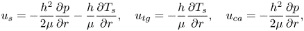 \begin{equation} u_{s} ={-}\frac{h^2}{2\mu} \frac{\partial p}{\partial r} - \frac{h}{\mu} \frac{\partial T_{s}}{\partial r},\quad u_{{tg}}={-}\frac{h}{\mu} \frac{\partial T_s}{\partial r},\quad u_{{ca}}={-}\frac{h^2}{2\mu} \frac{\partial p}{\partial r}, \end{equation}
where h is the location of liquid–gas interface, p is the pressure in the liquid phase and  $T_{s}$ is the interfacial temperature (liquid–gas), all from the numerical results.
Figure 5 maps the relative strength of thermal Marangoni flow and capillary flow in the short steady spreading stage, when the flow state becomes stable and the velocity ratio does not change much (stage  ${\unicode{x2462}}$ as in figure 3), $| u_{tg,max}|/|u_{ca,max}|$, for a wide range of combinations of $Ja^*$ and $Bi$, along with decomposed interfacial velocity (figure 5a–e). With decreasing $Bi$ from figure 5(d) to (b) to (e), the thermal Marangoni flow enhances and outweighs the capillary effect. As a result, the direction of interfacial flow reverses at a position close to the contact line, forming a SP as marked in figure 5(b,e).
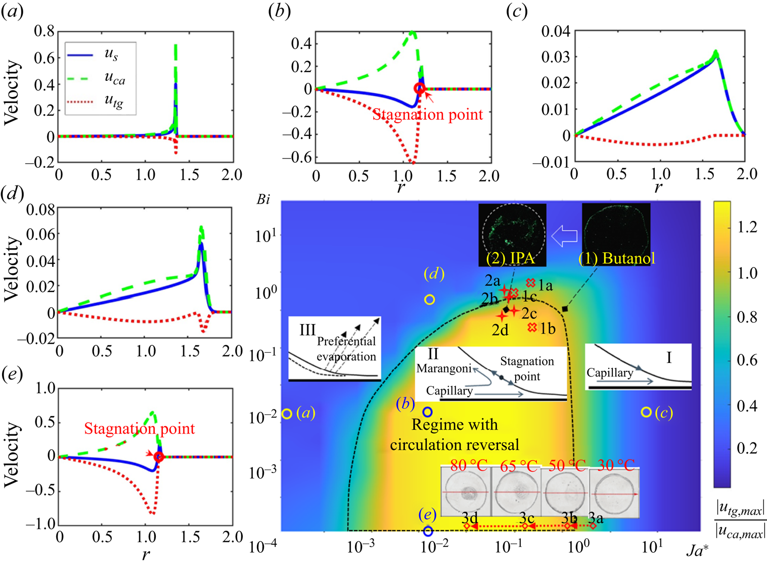
Figure 5. Phase diagram for the relative strength of thermal Marangoni flow to capillary flow. (a–e) Decomposition of surface velocity  $u_{s}$ to thermal Marangoni velocity $u_{tg}$ and capillary velocity $u_{ca}$, corresponding to letters (a–e) in the colourmap. Sketches I, II and III indicate the dominating mechanism at different regimes of the phase diagram. The experimental data by Xu et al. (Reference Xu, Luo and Guo2010) (1a, water on glass of thickness 1 mm; 1b, water on glass of thickness 0.15 mm; 1c, IPA on glass of thickness 1 mm), Ristenpart et al. (Reference Ristenpart, Kim, Domingues, Wan and Stone2007) ( $2\ \mathrm {\mu }\textrm {l}$ droplets of: 2a, methanol; 2b, ethanol; 2c, IPA; 2d, chloroform; on PDMS of thickness 4 mm) and Li et al. (Reference Li, Lv, Li, Quéré and Zheng2015) (3a to 3b with leftward dotted arrows and representative deposition patterns: $2.5\ \mathrm {\mu }\textrm {l}$ droplets on glass substrate of 30, 50, 65 and $80\,^\circ \textrm {C}$) are marked out, which indicate the flow reversal inside the droplet with changing environmental settings. Note that the dotted line presents the criterion for the formation of SP, and does not necessarily correspond to the contour line of $|u_{tg,max}|/|u_{ca,max}|=1$.
From figure 5(a) to (b) to (c), the value of  $Ja^*$ increases, corresponding to decreasing liquid volatility. At a small value of $Ja^*$, severe liquid–vapour phase change takes place, preferentially at the contact line region, leading to the concentrated interplay of Marangoni and capillary effects near the contact line (figure 5a). The severe interfacial phase change also leads to uniformly cold droplet surface, corresponding to weak Marangoni effect. At large value of $Ja^*$ (figure 5c), the whole process is close to isothermal due to weak evaporation. In such cases, the thermal Marangoni flow is also weak, and the droplet spreading is dominated by capillary flow, close to the case described by Tanner's law.
Overall, the thermal Marangoni effect becomes apparent and even outweighs the capillary effect at limited combinations of  $Ja^*$ and $Bi$. In regime II circled by dotted lines in figure 5, the thermal Marangoni effect is strong enough to reverse the flow direction and form a SP at the droplet surface. The droplet dynamics within this regime is therefore a joint result of the thermal Marangoni effect, evaporation effect and capillary effect, in contrast to the high- $Ja^*$ regime where capillary effect dominates (regime I) and the low- $Ja^*$ regime where liquid depletion due to evaporation near the contact line plays a significant role (regime III).
Previous studies, mostly experimentally, revealed the circulation reversal in evaporating droplets with varying substrate conductivity. We recalculated the experimental data in these pioneer work (Ristenpart et al. Reference Ristenpart, Kim, Domingues, Wan and Stone2007; Xu et al. Reference Xu, Luo and Guo2010), which are demonstrated in the phase diagram and show good correspondence with our theoretical predictions. Due to technical limitations, liquids in those studies are limited to water and alcohols where the evaporation is moderate with sufficient time for observation, and the substrates are mostly glass for microPIV visualisation. With the criterion proposed in figure 5, we are able to quickly find out the flow state for liquids with varying thermal conductivity and volatility, and on substrates with varying thickness and thermal properties, which could not have been possible solely based on experimental observations.
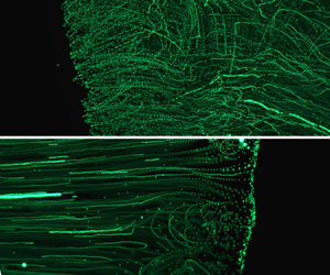
We additionally visualised the flow field near the bottom of droplets with different volatility (Supplementary movie 3). For less-volatile butanol, continuous outward flow is observed driven by the capillary force, which forms a ‘coffee ring’ as the droplet dries out (figure 6a). As the liquid volatility increases (IPA), the PIV particles tend to change its direction at a position near the three-phase contact line (SP), where a turning point in the tracing track of fluorescent particles is observed as in figure 6(b). The direction change avoids particle accumulation at the periphery, which leads to more uniform deposition patterns as the droplet fully dries out. The transition of flow direction and the formation of deposition patterns correspond with our numerical predictions by locating the  $Ja^*$– $Bi$ coordinates for (1) butanol–1.1 mm slide glass and (2) IPA–1.1 mm slide glass in figure 5. In correspondence to the flow direction, the deposition transits from coffee ring to more uniform patterns as indicated by the deposited fluorescent tracing particles from (1) butanol and (2) IPA droplets in figure 5.
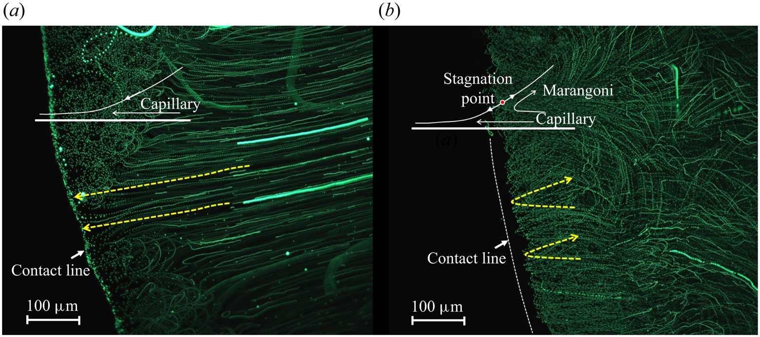
Figure 6. Flow pattern near three phase contact line visualised by tracer particles where the tracing tracks of fluorescent particles are overlap of 100 continuous frames: (a) a 0.5 $\ \mathrm {\mu }\textrm {l}$ butanol droplet on slide glass and (b) a 0.5 $\ \mathrm {\mu }\textrm {l}$ IPA droplet on slide glass.
In addition to the experiments in present work, the proposed phase diagram also correctly predicts the transition of deposition patterns from coffee ring (Deegan et al. Reference Deegan, Bakajin, Dupont, Huber, Nagel and Witten1997) to coffee eye with substrate heating (Li et al. Reference Li, Lv, Li, Quéré and Zheng2015), where the saturation vapour pressure increases and evaporation enhances with increasing substrate temperature, corresponding to decreasing  $Ja^*$ as indicated by diamond marks 3a to 3d along with leftward dotted arrows in figure 5. The phase diagram thus provides an efficient approach for quick prediction and control of deposition patterns in applications including printing, coating and thin film fabrication.
4.4. Spreading law of volatile droplets
The interfacial phase change and interacting flows further decide the spreading dynamics of the droplet. Specifically, the speed of contact line can be quantified with a power law in the form of  $R(t) = t^n$, where n is the spreading exponent. We then check the flow state and evaluate the corresponding spreading rate for a wide range of $Ja^*$ and $Bi$. A phase diagram is thereafter derived with representative cases shown in figure 7.
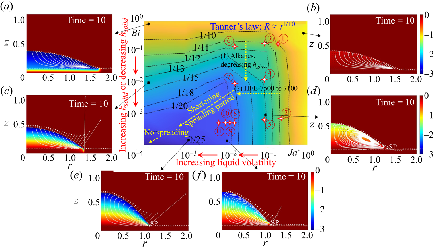
Figure 7. Phase diagram for the spreading rate of droplets along with demonstrations of flow and temperature fields in representative conditions. Contour lines of the spreading exponent are marked out with corresponding values. Experimental results by Shiri et al. (Reference Shiri, Sinha, Baumgartner and Cira2021) ((1) alkanes on glass substrates with decreasing thickness) and Kumar et al. (Reference Kumar, Parimalanathan, Rednikov and Colinet2022) ((2) HFE 7500 to 7100 with increasing volatility) are presented with yellow dotted arrows. Experimental results in our research are marked with stars numbered as  ${\unicode{x2460}}$ butanol on 1.1 mm glass, ${\unicode{x2461}}$ butanol on 1.0 mm copper, ${\unicode{x2462}}$ IPA on 1.1 mm glass, ${\unicode{x2463}}$ IPA on 1.0 mm SUS430, ${\unicode{x2464}}$ IPA on 1.0 mm copper, ${\unicode{x2465}}$ FC-72 on 1.1 mm glass, ${\unicode{x2466}}$ FC-72 on 1.0 mm SUS430, ${\unicode{x2467}}$ FC-72 on 1.0 mm copper ( ${\unicode{x2460}}\unicode{x2013} {\unicode{x2467}}$ are cases with substrate temperature $T_{sub}= 20\,^\circ \textrm {C}$), ${\unicode{x2468}}$ FC-72 on 1.0 mm copper ( $T_{sub} = 25\,^\circ \textrm {C}$), ${\unicode{x2469}}$ FC-72 on 1.0 mm copper ( $T_{sub}= 35\,^\circ \textrm {C}$) and ${\unicode{x246A}}$ FC-72 on 1.0 mm copper ( $T_{sub} = 45\,^\circ \textrm {C}$).
Overall, the spreading exponent decreases from 1/10 (Tanner's law) to smaller values ( $1/11, 1/12, \ldots, 1/25$) with decreasing $Ja^*$ and decreasing $Bi$. As $Bi$ decreases, heat transport across the substrate gets efficient and the thermal resistance in the liquid phase becomes dominant. This strengthens both the evaporation mass flux and the thermal Marangoni flow (enlarged temperature gradient), both of which retard droplet spreading.
With decreasing  $Ja^*$, the evaporation effect enhances, whereas the thermal Marangoni flow strengthens first (from isothermal state to large temperature gradient) and then weakens (as the droplet surface uniformly cools due to the strong evaporation cooling effect). The joint effect of non-uniform evaporation and thermal Marangoni flow shows in the slow down of droplet spreading with decreasing $Ja^*$. In addition, the influence of substrate thermal properties on the spreading rate is weak at small liquid volatility and becomes significant at high liquid volatility as the evaporation cooling effect strengthens and the efficiency of heat supply becomes eminent.
To validate our theoretical findings, a series of experiments were conducted with selected liquids and solid substrates. To ensure uniform spreading and minimise hysteresis, we prepared substrates with mirror finishing with the downward-side substrate temperature controlled as  $20\pm 0.2\,^\circ \textrm {C}$. Experiments were conducted with 1-butanol ( $p_{sat,20\,^\circ \textrm {C}} = 580\ \textrm {Pa}$), 2-propanol (IPA, $p_{sat,20\,^\circ \textrm {C}} = 4420\ \textrm {Pa}$) and FluorinertR (FC-72, $p_{sat,25\,^\circ \textrm {C}} = 30\,900\ \textrm {Pa}$), each with one order of magnitude higher saturation vapour pressure, and on different substrates, i.e. glass ( $k_{glass} = 0.8\ \textrm {W}\ \textrm {m}^{-1}\ \textrm {K}^{-1}$, $h_{glass} = 1.1\ \textrm {mm}$), SUS430 ( $k_{SUS430} = 25\ \textrm {W}\ \textrm {m}^{-1}\ \textrm {K}^{-1}$, $h_{SUS430} =1.0\ \textrm {mm}$), copper ( $k_{copper} = 398\ \textrm {W}\ \textrm {m}^{-1}\ \textrm {K}^{-1}$, $h_{copper} = 1.0\ \textrm {mm}$), each with one order of magnitude higher thermal conductivity. We also tried to further enhance the evaporation effect by increasing the downward side temperature of the substrate to $25\,^\circ \textrm {C}$, $35\,^\circ \textrm {C}$ and $45\,^\circ \textrm {C}$. The calculated values of $Ja^*$ and $Bi$ for cases ${\unicode{x2460}}$ to ${\unicode{x246A}}$ are summarised in table 3, which correspond with the data points marked in the phase diagram in figure 7.
Table 3. Values of  $Ja^*$ and $Bi$ for cases ${\unicode{x2460}}$ to ${\unicode{x246A}}$ (expressed in scientific notation).

In the experiments, the droplet is deposited onto the substrate right after its generation from the syringe, however close the distance between the droplet and the substrate is, it unavoidably has inertia (non-zero initial velocity) that pushes the contact line forwards. This stage when inertia effect dominates exhibits higher spreading rate, e.g.  $R\sim t^\alpha$, $\alpha = 1/4\sim 1/2$, typically between 0.1 and 10 ms (Ding & Spelt Reference Ding and Spelt2007; Bird et al. Reference Bird, Mandre and Stone2008; Chen et al. Reference Chen, Bonaccurso and Shanahan2013). As the droplet relaxes, viscous dissipation within the droplet becomes the main source resisting spreading, and the spreading radius follows Tanner's law, $r \sim t^{1/10}$, for non-volatile liquids (Tanner Reference Tanner1979). In the proposed research, we focus on the ‘Tanner's regime’ (or inertia-free regime) and investigate the influence of substrate conductivity and liquid volatility on this stage of spreading. This requires us to do linear fitting to log–log plot for droplet spreading after 10 ms from its deposition (green regions as in figure 8).

Figure 8. (a) Spreading behaviours of droplets at substrates with different thermal conductivity ( $T_{sub} = 20\,^{\circ }\textrm {C}$): ${\unicode{x2460}}$ IPA on 1.1 mm glass, ${\unicode{x2461}}$ IPA on 1.0 mm SUS430, ${\unicode{x2462}}$ IPA on 1.0 mm copper, ${\unicode{x2463}}$ butanol on 1.1 mm glass, ${\unicode{x2464}}$ butanol on 1 mm copper. (b) Spreading behaviours of droplets with different volatility on 1.0 mm copper substrate: ${\unicode{x2461}}$ butanol at $T_{sub} = 20\,^{\circ }\textrm {C}$, ${\unicode{x2464}}$ IPA at $T_{sub} = 20\,^{\circ }\textrm {C}$, ${\unicode{x2467}}\unicode{x2013} {\unicode{x246A}}$ FC-72 at $T_{sub} = 20\,^{\circ }\textrm {C}$, $25\,^{\circ }\textrm {C}$, $35\,^{\circ }\textrm {C}$, $45\,^{\circ }\textrm {C}$. These cases correspond with the mark numbers in figure 7.
Figure 8(a) compares the spreading rate of droplets at different substrate conductivity. By changing the substrate material from glass to SUS430 and to copper, the slope of the variation curve decreases, indicating a decreasing trend of spreading rate with increasing substrate conductivity ( ${\unicode{x2460}}\to {\unicode{x2461}}$, ${\unicode{x2462}}\to {\unicode{x2463}}\to {\unicode{x2464}}$).
The effect of liquid volatility on the spreading dynamics of the droplet is stronger than that of the substrate conductivity, as indicated by figure 8(b). For FC-72 droplets, a slight fluctuation (spread and contract) takes place at the very initial moment ( $< 10\ \textrm {ms}$) as a result of inertia effect (the inertia effect can cause a slight fluctuation as the surface tension of FC-72 is small, even though the distance for deposition is controlled to be as small as possible). The droplet then spreads, slows down and recedes after several hundred milliseconds. Here we focus on the short spreading period marked as green regions in figure 8(b).
With increasing liquid volatility, we can see an apparent decrease in the spreading rate ( ${\unicode{x2461}}\textrm { Butanol}\to {\unicode{x2464}}\textrm { IPA}\to {\unicode{x2467}}\textrm { FC-72}$ in figure 8b). By further increasing the substrate temperature, the spreading rate further decreases and the period of spreading shortens as indicated by ${\unicode{x2467}}$ $20\,^\circ \textrm {C}\to {\unicode{x2468}}$ $25\,^\circ \textrm {C}\to {\unicode{x2469}}$ $35\,^\circ \textrm {C}\to {\unicode{x246A}}$ $45\,^\circ \textrm {C}$ in figure 8(b). For substrate temperature higher than $45\,^{\circ }\textrm {C}$ ( $T_{FC\textrm {-}72, boiling} = 56\,^\circ \textrm {C}$ ), the spreading stage is no longer distinguishable and no apparent spreading can be observed, i.e. the contact line recedes right after the droplet deposition due to significant mass loss at the contact line region, representing a general scenario in flash evaporation.
We further apply the calculated dimensionless numbers to the proposed model, and get the spreading component at the steady spreading stage. Very nice quantitative correspondence is found between experimental and theoretical values as summarised in table 4. Here, the experimental liquids and substrates cover most of the cases that span from non-volatile to the most-volatile liquids in practical applications and on substrates with a full range of thermal conductivity, thus allowing for reliable prediction of the liquid behaviours by quickly locating its  $Ja^*$– $Bi$ coordinate in the phase diagram.
Table 4. Experimental (Exp.) spreading exponent n in comparison with the numerical (Num.) value by matching its position ( $Ja^*$, $Bi$) in the phase diagram. Numbers ${\unicode{x2460}}\unicode{x2013} {\unicode{x246A}}$ correspond with the cases marked in figure 7. Deviations between experimental and numerical results exist mainly in the high-volatility and low-substrate-conductivity region (small $Ja^*$ and large $Bi$, e.g. case ${\unicode{x2465}}$), where the heat dissipation into the gas phase is no longer negligible.
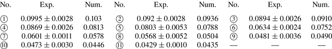
Besides the experiments in present research, our conclusions on the effect of substrate thermal properties correspond with the work of Shiri et al. (Reference Shiri, Sinha, Baumgartner and Cira2021) where alkane droplets indicate increasing contact angle and slowing-down spreading rate as the thickness of the glass substrate decreases stepwise from 6 mm to 0.063 mm. The influence of liquid volatility also meets with a very recent work by Kumar et al. (Reference Kumar, Parimalanathan, Rednikov and Colinet2022) where the spreading rate of HFE-7500 to HFE-7100 droplets decreases with increasing liquid volatility (decreasing chain length). These uniform findings allow for optimal design of working fluids and substrates in phase change thermal management and dry-out prevention for high-power-density electronics, which requires a balance between liquid wetting and thermal efficiency.
5. Conclusions and perspectives
In this research, we have revisited the classical problem of droplet wetting with interfacial phase change, which is of fundamental importance to a wide range of industrial processes that involve three phases. The objective originates from the urgent need for a unified explanation to a couple of basic scientific problems including the flow transition for different liquid–solid combinations, the existence of SP near the three phase contact line, the relative strength of capillary and Marangoni flows, the deposition patterns from colloidal suspensions, as well as the corresponding spreading dynamics in diverse scenarios. Due to the requirement for substrate transparency and the available frame rate of existing visualisation techniques, explorations on these scientific issues are limited to substrates such as glass, and common liquids such as water and alcohol, whereas important liquids and substrates in the vast industrial fields are less explored, such as refrigerants and metallic substrates. This requires a close collaboration between experimental and numerical efforts, where information that cannot be revealed from one side can be disclosed by the other.
Here, we have developed a lubrication-type model that considers the non-isothermal heat conduction into the solid substrate. We have further conducted experiments on the flow field and the spreading rate for a wide range of combinations of liquids and solids. With one-to-one comparison between the numerical and experimental results, we have elucidated the key dimensionless numbers that come into effect, i.e. the Jakob number,  $Ja$, the liquid–solid Biot number, $Bi$, and the Marangoni number, $Ma$. Unified criteria have been proposed for the transition of flow state, and we have provided unbiased explanations to a series of individual works on deposition patterns from drying droplets. A phase diagram for spreading dynamics has further been established along with experimental demonstrations, which extend Tanner's law (for non-volatile liquids in an isotherm state) to a full range of liquids with saturation vapour pressure spanning from $10^1$ to $10^4$ Pa and on substrates with the entire range of thermal conductivity spanning from $10^{-1}$ to $10^3\ \textrm {W}\ \textrm {m}^{-1}\ \textrm {K}^{-1}$.
In the theoretical aspect, this work has illustrated the relative strength of interacting physical mechanisms as regimes I, II and III in figure 5, where the capillary effect dominates at low liquid volatility in regime I, the Marangoni effect, capillary effect and evaporation effect interact in regime II and the strong evaporation effect (preferential mass loss near contact line) dominates in regime III at very high liquid volatility. Such decomposition of the mechanisms allows for quick positioning of the influencing factors, and enables efficient control of liquid behaviours in various phase change energy devices, printing–coating processes and microfluidic systems.
Overall, Tanner's law describes the spreading of non-volatile Newtonian fluids on smooth solid substrates. Here ‘non-volatile’, ‘Newtonian’ and ‘smooth’ are necessary conditions for the universality of the spreading exponent. With interfacial phase change (volatile liquids), the process becomes non-isothermal in which case the non-uniform distribution of mass flux and the thermal Marangoni effect come into play along with the capillary and viscous effect, as quantified in the present work. For non-Newtonian fluids, the viscosity largely depends on the shear stress. Theories for the spreading dynamics of dilatant fluids (shear thickening) and pseudo-plastic fluids (shear thinning) were established in previous studies based on the lubrication approximation (Rafaï et al. Reference Rafaï, Bonn and Boudaoud2004; Wang et al. Reference Wang, Lee, Peng and Lai2007a) and experiments (Wang et al. Reference Wang, Zhang, Lee and Peng2007b), and the explorations are still ongoing. For topological surfaces with microstructures, the spreading dynamics can be more complex. A systematic understanding is yet reached due to the diverse surface topology and the complex liquid–solid interaction, where the small-scale surface structure affects the dynamics of the contact line and thereafter the overall droplet behaviours. By taking advantage of the asymmetric effect of surface topology, it is also possible to realise directional fluid motion, which indeed has been widely exploited in recent years with promising applications in directional liquid transport (Li et al. Reference Li, Zhou, Li, Che, Yao, McHale, Chaudhury and Wang2017; Li, Li & Dong Reference Li, Li and Dong2020), water harvesting (Zheng et al. Reference Zheng, Bai, Huang, Tian, Nie, Zhao, Zhai and Jiang2010; Dai et al. Reference Dai, Sun, Nielsen, Stogin, Wang, Yang and Wong2018) and dry-out prevention (Li et al. Reference Li, Zhou, Tao, Zheng and Wang2021).
Supplementary movies
Supplementary movies are available at https://doi.org/10.1017/jfm.2024.385.
Funding
The authors gratefully acknowledge the support received from Japanese Society for the Promotion of Science (JSPS), and ThermaSMART project of European Commission (grant no. EC-H2020-RISE-ThermaSMART-778104). Z.W. and C.I. acknowledge the support from JSPS KAKENHI (grant nos JP21K14097, JP21H01251, JP22K18771, JP24K17218).
Declaration of interests
The authors report no conflict of interest.


 Open access