


1. Introduction
1.1 Global inequalities
‘The rich get richer’ is an expression dating back to the early 19th century poet Percy Bysshe Shelley (Shelley, Reference Shelley2009). Two hundred years later, Thomas Piketty demonstrated that this is not only poetic wordplay but a working principle of the capitalist system as it stands today (Piketty & Saez, Reference Piketty and Saez2014). The return on capital that the very wealthy profit from is much higher than aggregate economic growth and the wage growth of the general public. As a consequence, the gap between rich and poor is widening (Alvaredo et al., Reference Alvaredo, Chancel, Piketty, Saez and Zucman2018).
There is no country where income inequality has a Gini coefficient below 0.25: most are above 0.3 and a large number of countries exists with Gini coefficients above 0.4 (World Bank, 2020c). Even at the lowest Gini coefficients of around 0.25, as for example in the case of Sweden, the top 10% income earners of the population may hold ~23% of total income and the bottom 10% only ~3% (World Bank, 2020d). National income inequality is also correlated with various other inequality dimensions, for instance the rural–urban divide, gender inequality and racial inequality (Ma et al., Reference Ma, Wang, Chen and Zhang2018; Ortiz-Ospina & Roser, Reference Ortiz-Ospina and Roser2018).
Nevertheless, income inequality is largest when measured at the international level, despite at least one decade of global income convergence between countries (Milanovic, Reference Milanovic2013). The global Gini coefficient of income is estimated to be between 0.6 and 0.7 (Anand & Segal, Reference Anand and Segal2008; Milanovic, Reference Milanovic2013). This is more than in any single country.
The global divide does not end with prosperity and affluence. It also has been repeatedly shown that environmental footprints scale with income level (Ivanova et al., Reference Ivanova, Stadler, Steen-olsen, Wood, Vita, Tukker and Hertwich2015; Moran et al., Reference Moran, Kanemoto, Jiborn, Wood, Többen and Seto2018; Wiedenhofer et al., Reference Wiedenhofer, Lenzen and Steinberger2013, Reference Wiedenhofer, Guan, Liu, Meng, Zhang and Wei2017). Energy consumption is coupled to income and so are carbon emissions (Oswald et al., Reference Oswald, Owen and Steinberger2020; Teixidó-Figueras et al., Reference Teixidó-Figueras, Steinberger, Krausmann, Haberl, Wiedmann, Peters, Duro and Kastner2016). Affluence is now widely considered the largest driver of resource use and environmental degradation (Wiedmann et al., Reference Wiedmann, Steinberger, Lenzen and Keyßer2020). This is why the global income distribution is directly linked to the climate emergency and other ecological crises. High-income countries contribute by far the most to emissions, as do high-income individuals within countries. Conversely, low-income households and communities often struggle to afford basics such as clean cooking fuel, lighting and food storage (Rao & Pachauri, Reference Rao and Pachauri2017). Low-income countries in the Global South are also those most affected by climate change (Byers et al., Reference Byers, Gidden, Leclere, Balkovic, Burek, Ebi, Greve, Grey, Havlik, Hillers, Johnson, Kahil, Krey, Langan, Nakicenovic, Novak, Obersteiner, Pachauri, Palazzo and Riahi2018). Southern island states and coastal mega-cities are vulnerable to sea level rise, and extreme heat in Sub-Saharan Africa is already discussed as a cause for armed conflicts (O'Loughlin et al., Reference O'Loughlin, Witmer, Linke, Laing, Gettelman and Dudhia2012; Sen Roy, Reference Sen Roy and Sen Roy2018). Additionally, developing countries often lack the economic resources to adapt to climate change (Mertz et al., Reference Mertz, Halsnæs, Olesen and Rasmussen2009).
The distribution of economic wealth around the globe emerges as a key not only to the biggest problems of our time, but also to their solutions. If wealthy countries were to reduce their affluence, they would lessen the burden on the environment. As of today, no country is actively pursuing such a degrowth strategy (Hickel, Reference Hickel2019c). This is despite evidence demonstrating that well-being is only coupled to affluence up to a certain level, beyond which no significant gains in well-being are made (Easterlin, Reference Easterlin1972; Fanning & Neill, Reference Fanning and Neill2019; Steinberger et al., Reference Steinberger, Lamb and Sakai2020). Expressed in terms of gross domestic product (GDP) and allowing for simplification, the gain in well-being indicators (life expectancy, life satisfaction, etc.) is relatively small after roughly $15,000 purchasing power parity (PPP) per capita – a level only modestly larger than the global average (although maxima are achieved at higher levels; Jebb et al., Reference Jebb, Tay, Diener and Oishi2018). If poor countries were to increase their prosperity, however, they would likely see a rapid increase in well-being, including an across-the-board surge in health indicators and adoption of clean technologies such as electric cooking stoves (Vigolo et al., Reference Vigolo, Sallaku and Testa2018).
Besides the ambivalent relationships between income, the environment and well-being, there are also studies that point to the degree of inequality itself as a critical social parameter. Arguments have been made that inequality affects the very fabric of society: the mental health of people. Evidence points to relationships between inequality and crime, obesity, educational outcomes and so forth (Wilkinson & Pickett, Reference Wilkinson and Pickett2009). More equal nations consistently perform best across indicators.
Despite continually growing evidence of the critical importance of inequality in shaping environmental and social outcomes, there is little research quantifying the potential consequences of alternative distributions (Melamed & Smithyes, Reference Melamed and Smithyes2009). What would be the consequences of altering the distribution of income across the globe? How would this impact poverty and ecology? How would it reshape international relations? Is it even possible to keep the global economy the same size, redistribute and achieve better social outcomes and less environmental impact? These are big questions that can be addressed in many ways. Here, we want to make a simple but novel contribution: simple in its approach, but novel in its quantification of radically different income distributions and their consequences. We model alternative distributions of global income (GDP per capita) and study the effect on final energy consumption of households.
1.2 Energy and human life
Why final energy consumption of households? Energy is a universal quantity pervading physical, biological, economic and social processes. It is the services that energy provides that people make use of to meet their needs (Fell, Reference Fell2017; Kalt et al., Reference Kalt, Wiedenhofer, Görg and Haberl2019). Final energy is closer to these end-use services than primary energy. Between energy and well-being exists a similar saturating relationship as between income and well-being, with high levels of energy consumption not contributing much to well-being (Brand-Correa & Steinberger, Reference Brand-Correa and Steinberger2017). Nevertheless, a minimum quantity applied in the right way is absolutely crucial in achieving a high quality of life: this minimum has recently been referred to as ‘decent living energy’ (DLE) (Rao & Min, Reference Rao and Min2018a). The DLE level has been quantified with estimates pointing to somewhere between 10 and 40 Gigajoule per capita per year (GJ/capita/yr) depending on what kind of technology is assumed, the location dealt with and what is assumed to be essential for well-being (Goldemberg et al., Reference Goldemberg, Johansson, Reddy and Williams1985; Rao et al., Reference Rao, Min and Mastrucci2019a; Steinberger & Roberts, Reference Steinberger and Roberts2010).
A recently estimated global average for DLE is around 15 GJ/capita/yr when very advanced technologies are deployed worldwide (Millward-Hopkins et al., Reference Millward-Hopkins, Steinberger, Rao and Oswald2020), rising to 26 GJ/capita/yr when somewhat less advanced technologies are assumed (but still significantly more efficient than currently prevailing ones). Indeed, energy consumption at any level in no way guarantees a decent living standard, since it is the quality and composition of energy services achieved which ultimately matter. Energy consumption can be inefficient and misapplied. However, for the purposes of this study, we will use 26 GJ/capita/yr as a reasonable threshold for energy poverty. It is important to note that we focus purely on household consumption-related energy footprints: we do not include energy used for government expenditure or capital formation. In DLE estimates, however, this collective form of energy actually plays a substantial role. It sometimes constitutes up to a third of DLE estimates. As a consequence, 26 GJ/capita/yr for DLE is a conservative estimate for household energy alone and a good first order approximation. A major advantage of household energy is that we can clearly associate it with different income groups. This is not so straightforward with government and capital formation-related energy.
Real-world energy consumption of course is much more varied, with a large amount of people living below this threshold and an affluent, largely western, economic elite consuming drastically more energy. The global range of final energy consumption spans roughly 1–300 GJ/capita/yr (Oswald et al., Reference Oswald, Owen and Steinberger2020), but this is without considering the super-rich who likely attain energy footprints in excess of 1000 GJ/capita/yr (Oswald et al., Reference Oswald, Owen and Steinberger2020; Otto et al., Reference Otto, Kim, Dubrovsky and Lucht2019). In short, there is both extreme energy poverty and severe energy excess on the same planet. Although far from perfect, final energy consumed by households is one of the best indicators for living standards and for the biophysical impact of people, encompassing what is necessary to achieve a decent life and pure luxury. This makes final energy consumed by households an attractive consequential indicator. We use it to observe and judge redistributional outcomes.
1.3 Energy, inequality and scenarios
Models of energy systems have for a long time not been considerate of income distribution but worked on the basis of a single representative household (Rao et al., Reference Rao, Van Ruijven, Riahi and Bosetti2017; van Soest et al., Reference van Soest, van Vuuren, Hilaire, Minx, Harmsen, Krey and Luderer2019). Recently, there have been various efforts to integrate income distribution into general equilibrium models and in particular energy system scenarios (van Ruijven et al., Reference van Ruijven, van Vuuren, de Vries, Isaac, van der Sluijs, Lucas and Balachandra2011, Reference van Ruijven, O'Neill and Chateau2015). Yet, they mostly project change to happen on the basis of large-scale diffusion of innovation or efficiency gains (Grubler et al., Reference Grubler, Wilson, Bento, Boza-kiss, Krey, Mccollum and Valin2018; Rogelj et al., Reference Rogelj, Huppmann, Krey, Riahi, Clarke, Gidden and Meinshausen2019) and energy demand is often only made income-granular after the simulations. Most importantly, if income distributions are integrated in models they remain close to the empirically observable and plausible under current or planned policies (Trutnevyte et al., Reference Trutnevyte, Hirt, Bauer, Cherp, Hawkes, Edelenbosch, Pedde and van Vuuren2019; van Ruijven et al., Reference van Ruijven, O'Neill and Chateau2015) and at times even assume constant distributions for future projections. Studies more explicitly addressing the implications of radically alternative income or wealth distributions for energy demand are so far missing. There are now projections of income inequality into the future (Rao et al., Reference Rao, Sauer, Gidden and Riahi2019b) but whenever inequalities in energy and emissions decline in future scenarios, it is a by-product of catch-up economic growth in developing countries and efficiency gains in developed ones. It often is an extrapolation of past technological trends and growth trajectories (Bauer et al., Reference Bauer, Calvin, Emmerling, Fricko, Mouratiadou, Sytze, Boer, Berg, Carrara, Daioglou, Drouet, Edmonds, Gernaat, Havlik, Johnson, Klein, Kyle, Marangoni, Masui and Vuuren2017; Riahi et al., Reference Riahi, van Vuuren, Kriegler, Edmonds, O'Neill, Fujimori and Tavoni2017), not a consequence of economic redistribution. This approach to solving international energy inequality is very slow (Semieniuk & Yakovenko, Reference Semieniuk and Yakovenko2020), and given the scale and the urgency of transforming the economy and the energy system, it is arguably not adequate. Going beyond these studies, our purpose is to test the potentially large leverage of alternative income distributions to address energy development and climate.
Previous distribution-focused research includes several important studies. One is a scenario by Rao and Min (Reference Rao and Min2018b), who simulate income distributions jointly with other scenario parameters drawn from the shared socio-economic pathways (Bauer et al., Reference Bauer, Calvin, Emmerling, Fricko, Mouratiadou, Sytze, Boer, Berg, Carrara, Daioglou, Drouet, Edmonds, Gernaat, Havlik, Johnson, Klein, Kyle, Marangoni, Masui and Vuuren2017). They concluded that a reduction in inequality, if associated with growth in low-income countries and low growth in high-income regions, yields lower global carbon emissions. The result depends on assumptions about energy efficiency improvements in large economies such as India and China. Instead of further dwelling on technical aspects, they suggest examining the mechanisms of consumption for different income groups: Who consumes what, and why? In another recent study, equity policies have been implemented in a national-scale integrated assessment model (D'Alessandro et al., Reference D'Alessandro, Cieplinski, Distefano and Dittmer2020). The model focuses on the interactions of redistributive policies with other policies in several scenarios; most notably testing a green growth policy agenda and a degrowth one. The study concludes that under degrowth policies, greater equity and lower carbon emissions are compatible objectives, whereas under green growth, lower emissions are only possible at the cost of higher inequality. Two rare contributions that solely focus on the distribution of energy and carbon emissions have been made by Chakravarty et al. The first concluded that allowing a minimum floor of 3.7 tonnes/capita/yr CO2 emissions for the poor can be off-set by capping emissions of the 1 billion highest emitters (Chakravarty et al., Reference Chakravarty, Chikkatur, Coninck, De, Pacala, Socolow and Tavoni2009). The second modelled the global distribution of energy consumption and tested the implications of implementing a floor of 10 GJ/capita as well as projecting energy demand over time but did not consider redistribution itself (Chakravarty & Tavoni, Reference Chakravarty and Tavoni2013).
These studies report important findings but none of them has attempted what we do here: changing the global income distribution and studying the outcomes in energy terms. The goal of this study is not to propagate a naive or overly simplified political narrative. We do however believe that the case for a global income and energy redistribution is compelling enough in order to be taken seriously and studied accordingly.
1.4 On terminology: income, wealth, affluence or which one?
The term income can refer to several things. For example, it can refer to the income of a person or the income of a household subsuming different income sources, such as wages and return on capital. In an international context, when comparing countries, the term income is often equated with GDP per capita. There is also gross national income (GNI) which, in addition to the territorial measure of GDP accounts for value added by citizens abroad. GNI is less commonly used and the relationships between GDP, household expenditure and energy consumption are well established in the literature. In this study, we model the global distribution of GDP per capita per year, and thus we use the term income interchangeably with GDP per capita per year. From this, we derive expenditure of households (via the relationship depicted in Supplementary Figure S1) which is the money people spend on different goods and services. Wealth, on the contrary, is the sum of physical and financial assets somebody owns. The general terms affluence and prosperity combine income, expenditure and wealth. Affluence generally denotes excess, whereas prosperity has a more positive connotation referring to decent levels of well-being.
2. Methods
2.1 Methods and model overview
We model the global income per capita distribution in a simple but data-driven way by building on data by the World Inequality Lab and the World Bank. We elaborate on this in section 2.2. After modelling income, we estimate expenditure as a power law function of income, based on a log–log regression between the two. We then allocate expenditure between 14 different consumption categories, taken from Oswald et al. (Reference Oswald, Owen and Steinberger2020). The budget share of consumption categories, that is, the share of total expenditure that is allocated to a certain good or service, is determined by income elasticities of demand. These elasticities can also be interpreted as power law exponents and are derived from log–log regressions of expenditure per category on total expenditure (Steinberger et al., Reference Steinberger, Krausmann and Eisenmenger2010). The regressions are population-weighted cross-country models which avoids bias from very small countries or small population segments within countries (Steinberger & Roberts, Reference Steinberger and Roberts2010). The regressions cover 88 countries with each country including four to five income groups (~85% of the global population and ~85% of global GDP) resulting in a sample size generally around 350 or larger and spanning roughly 4 orders of magnitude of household expenditure groups, from roughly $100 to $100,000 PPP per year. The income elasticity of demand represents how much percentage the demand in a certain consumption category increases, when income increases by 1%. Each consumption category corresponds to an energy intensity (MJ/$) that is based on final energy footprint accounts in Oswald et al. (Reference Oswald, Owen and Steinberger2020). The energy intensity either represents the direct final energy used at home (as in the category ‘heating or electricity’), or the indirect final energy that is embodied in the entire supply chain of a good (as in the case of the category ‘food’). Energy intensities are the aggregate global final energy intensities of household consumption, so global final energy per category over global household expenditure per category, and thus constant and homogenous across the income distribution. The average energy intensity per income group varies because of differences in the composition of expenditure across income, see Supplementary Figure S2 for details. Of course, in reality, energy intensities are dynamic and evolve over time, particularly so during the ongoing global energy transition and efforts in efficiency and decarbonization. This means that in the future energy intensities across consumption categories may change incrementally or drastically, and thus the technological conditions underlying redistribution scenarios may be altered. Our static model reproduces the fundamentals of technology as observed in 2011, with high energy intensities occurring mostly in direct energy consumption such as residential energy or fuel and lower energy intensities of indirect energy consumption – a pattern that is very likely to be persistent.
The consumption elasticities are held constant as well, which is a simplifying assumption, since income elasticities of demand have been shown to vary across income levels (Harold et al., Reference Harold, Cullinan and Lyons2017). Yet, at the minimum, the power laws employed capture the average global trend of consumption and, since the equations are non-linear, they account for variation in budget allocation. We tested for non-constant elasticities (evolving with income levels) but did not find trends that are sufficiently significant, see Supplementary Table S4. The constant elasticities are based on the most reliable regression models we tested and are consistent with constant energy intensities.
A full list of consumption categories, energy intensities and elasticities can be found in Supplementary Table S2. Figure 1 illustrates the basic flow of the model; from income distribution to final energy footprint accounts. It also depicts at what stages of the model we ‘intervene’ and explore its behaviour: in sections 3.1 and 3.2 we redistribute income by varying the parameters of the income distribution (first we vary the standard deviation and then we set floors and ceilings) and in section 3.3 we evaluate the uncertainty inherent to the model, by employing a simple Monte Carlo simulation on the elasticities and energy intensities.

Fig. 1. Model flowchart.
A crucial feature of our model is that global GDP is constant before and after redistribution. Another fixed parameter is population. The expenditure and energy demand resulting from changes in the income distribution, however, are not preserved and change with the model parameters. The model is static; we consider the year 2011 only. This is deliberate as we wish to isolate the effect of distribution from the influence of other variables, which would inevitably change over time. The simulations should be considered ‘computational experiments’ that test the effect of redistribution under certain experimental conditions and holding everything else constant. The model is implemented in Python Anaconda and all code and data can be accessed on https://github.com/eeyouol. Table 1 summarizes all major assumptions of the model.
Table 1. Major assumptions of the model

2.2 Modelling the global income distribution
The global income distribution has been estimated many times (Anand & Segal, Reference Anand and Segal2008; Lakner & Milanovic, Reference Lakner and Milanovic2016; Liberati, Reference Liberati2015) and recent data are from Alvaredo et al. (Reference Alvaredo, Chancel, Piketty, Saez and Zucman2018). They estimate the income distribution in terms of per adult equivalent national income and EURO PPP. We converted this distribution into dollar GDP PPP per capita, via a coefficient representing the currency exchange rate and a ‘working-age population’ factor for the translation of the adult equivalent scale to the per capita one (World Bank, 2020a). In addition, we estimated the global distribution of GDP per capita ourselves based on household expenditure data in Oswald et al. (Reference Oswald, Owen and Steinberger2020). We also consulted another estimate made by Lakner and Milanovic (Reference Lakner and Milanovic2013). We compare the cumulative distribution function of all estimates in Figure 2, finding their shapes to be similar, resembling an ‘S-curve’ when the x-axis is log-scale. The Lakner and Milanovic data display visibly lower incomes, but their data are for 2008 rather than for 2011 and concerns disposable household income, not GDP or pre-tax national income.

Fig. 2. Modelling the global income distribution. Lakner and Milanovic data have been adjusted from $PPP 2005 to $PPP 2011. Alvaredo et al. data have been adjusted from national income per adult equivalent €PPP to GDP per capita $PPP.
We fit a log-normal distribution to the adjusted data by Alvaredo et al. (Reference Alvaredo, Chancel, Piketty, Saez and Zucman2018) and fix its mean to the average global GDP per capita in 2011 (=13,592 USD PPP constant 2011) (World Bank, 2020b). This way we cover two essential properties of the distribution: (1) the shape of the distribution provided by Alverado et al. and (2) the global mean income provided by the World Bank. The log-normal fit to the adjusted data is almost perfect (R 2 of predicted cumulative population values >0.99) even though it does not exhibit the same long tails as the original data. It is missing out on the super-rich and people with nearly zero income. Nevertheless, the tails we are missing make up less than 0.1% of the population, and we cover a vast range of income groups from around $50 PPP to $500,000 PPP per capita. The log-normal model has advantages besides being a good fit to the data. For instance, it is defined via an easy-to-interpret set of parameters, the mean and the standard deviation of the logged GDP values (Cowell, Reference Cowell2009). There are other distributions suggested to better represent global income data such as Pareto-log-normal curves (Hajargasht & Griffiths, Reference Hajargasht and Griffiths2013) or generalized Pareto curves, particularly so in the heavy tails to the right (Blanchet et al., Reference Blanchet, Fournier and Piketty2017). Here, we do not attempt to model the income distribution perfectly but to develop a simple and useful model to investigate the relationship between income inequality and household energy consumption. Apart from our study focusing on the income–energy relationship, not the nature of the income distribution itself, there is no reliable data for income elasticities of demand or energy intensities among extremely high-income groups (≫$1 million/capita/yr). For our purposes, it is thus reasonable to restrict the model to the lognormal distribution without Pareto tails.
After determining the appropriate model, we solve the cumulative distribution function of the log-normal model for 1000 different groups, for the lowest 0.1%, the next 0.2% and so forth until reaching 100% of the population. Therefore, we obtain income data for 1000 distinct income groups globally. Each income group represents 0.1% of the global population or ~7 million people. We do not consider individual nations, and treat the whole distribution as one. The corresponding equations are standard and can be found in Supplementary Note 1.
3. Results
3.1 Simulation no. 1: varying the global income distribution
The first simulation varies the spread of the global income distribution but holds the global average income constant, at ~$13,600 PPP. In other words, the total size of the world economy is preserved at $95 trillion PPP but redistributed. The standard deviation (σ X) of the global income distribution is ~$26,800 PPP. We decrease this in linear steps down to a tenth of the original value ($2680 PPP) and up to twice the original ($53,600 PPP). This corresponds to global income Gini coefficients of 0.11 and 0.77, respectively. With these changes in income inequality (Figure 3a) we see changes in total energy inequality, whereas total global energy demand changes only modestly. Global demand decreases from 209 Exajoules (EJ) to 201 EJ (−3.8%), when increasing inequality, and increases up to 223 EJ (+6.7%) when decreasing inequality (Figure 3b). This is for two reasons: first, if inequality is decreased, the population approaches the mean value of the income distribution around ~$13,600 PPP. At this level of income, people generally spend a higher share of their total income than at higher levels. Second, there is a change in the composition of consumption. Figure 3 illustrates the considered ensemble of distributions in panel (a) and the implications for global energy demand in panel (b).

Fig. 3. Varying the global income distribution aggregate view. Panel (a) shows the ensemble of income distributions. The red thick line represents the current income distribution. Panel (b) illustrates the implications for aggregate global energy demand. It plots total energy demand on the y-axis against total income inequality on the x-axis (expressed as the standard deviation of global income). The secondary x-axis on top displays the corresponding income Gini coefficients. The relationship between these two axes is non-linear and can be found in Supplementary Figure S10. Total energy demand increases by more than 6% when inequality is lowered and decreases by nearly 4% if inequality is increased. The black dashed line represents the situation as of 2011.
The sectoral composition of energy demand also changes as a function of inequality. If income inequality is decreased, the overall energy demand shifts more to residential energy use, particularly towards heat and electricity. For the purpose of illustration, we aggregate the 14 consumption categories down to six categories in Figure 4. Food, wearables and other housing (which includes housing repairs, etc.) are for example put into one category called subsistence. Subsistence experiences a slight increase with more equality. Transportation-related energy, including fuel for vehicles, flights and public transport, is almost halved in a more equal world compared to a very unequal one (~38 EJ vs. 66 EJ respectively). The equal world consumes more domestic energy (~107 EJ) than the unequal one (~75 EJ). There is a symmetric trade-off between ‘at home’ and mobility. The sectoral shifts are rooted in redistributed income at a person level and expenditure moving from high-income individuals to lower income individuals.

Fig. 4. Varying the global income distribution detailed view. Panel (a) shows the composition of total global household energy demand as a function of the income standard deviation. Panel (b) shows the percentage amount of low-consumer population (orange line) and the percentage amount of energy mega-consumers (blue line) as a function of the standard deviation. Panel (c) shows the typical energy consumption profile of a person barely meeting the DLE threshold and an energy mega-consumer. All three panels are connected: the composition in panel (a) changes because of the structural shifts illustrated in panels (b) and (c). The black dashed lines represent the situation as of 2011.
Furthermore, with decreasing income inequality, we also see people being lifted out of energy poverty (estimated with respect to the previously discussed threshold of 26 GJ/capita/yr). The reduction in inequality must be drastic: to ensure less than 20% of population are living below 26 GJ/capita/yr, we need to decrease the spread of the distribution to a tenth of the current spread, corresponding to a Gini coefficient of 0.11. At the lowest tested inequality, the range of energy consumption is 10–56 GJ/capita/yr – corresponding roughly to low-income groups in Eastern Europe, and the second quintile in the UK or Germany, respectively. In this world, ~80% of the population falls between 26 and 40 GJ/capita/yr. A broader ‘energy middle class’ emerges. At the highest tested inequality, on the contrary, the range is 1–2000 GJ/capita/yr, with nearly 80% of the population falling below 26 GJ/capita/yr. For the sake of simple comparison, we define a ‘low consumer’ as someone who barely meets DLE (consumes 26–30 GJ/capita/yr) and define ‘mega consumer’ as people with a consumption of 270 GJ/capita/yr or more, which is equivalent to the amount the top 20% Americans consumed in 2011. With increasing inequality, there are more mega-consumers and more people who do not meet DLE. At the highest inequality, for example, there are twice as many mega-consumers, constituting 1.2% of the global population compared to only 0.6% estimated to exist in the real-world of 2011. On the contrary, at the lowest inequality only around 10% live below DLE standards and there are no mega-consumers at all. Figure 4 illustrates the process with panel (a) showing the overall sectoral composition of demand as a function of inequality. Panel (b) displays the percentage of low consumers and mega consumers as a function of inequality, and panel (c) illustrates the ‘typical’ energy profile of a low consumer and a mega consumer.
Oswald et al. (Reference Oswald, Owen and Steinberger2020) demonstrated that it is crucial to go beyond total energy inequality, and to differentiate between consumption categories. For example, energy embodied in food and residential energy use are more equally distributed than energy for the purposes of mobility or for going on holidays. This is a critical consideration in the discourse around climate justice and climate change mitigation. Energy is related to emissions and other environmental hazards, such as resource extraction and pollution, for instance during oil or gas leaks. It is thus no surprise that the inequality in emissions is very similar to the one in energy (Ivanova & Wood, Reference Ivanova and Wood2020; Oswald et al., Reference Oswald, Owen and Steinberger2020). Consequentially, when a few people use a lot of energy and many people do not, the responsibility for environmental damage concentrates among a few. This pattern is tragic because most of the energy used by mega-consumers is not essential. It is ‘luxury energy’ and ‘luxury emissions’ which could, in many cases, be avoided without harming anyone (Shue, Reference Shue1993). The result is that some people use vast amounts of energy for luxury purposes, and others reap the negative externalities.
We investigate the correlation between income inequality and energy inequality differentiated by category. There are some categories that exhibit systematically higher energy inequality than income inequality, such as vehicle fuel, vehicle purchases and package holidays. Others such as food, heat and electricity are systematically more equal than income. As we increase income inequality, the inequality in luxury categories grows faster than the inequality in subsistence basics. When reducing income inequality to a Gini coefficient below 0.4, the energy metrics converge until they approach the level of income inequality. From a justice perspective, this means that only then do people bear more or less the same responsibility for energy externalities. Figure 5 plots the Gini coefficients in energy consumption (y-axis) vs. the Gini coefficient in income (x-axis). Supplementary Figure S5 depicts the corresponding absolute energy figures and the shares of the top 1% global income earners within the total energy consumption of a category. As an illustrative example of the scale of luxury externalities: among the top 1% income earners, we can be certain that most of the energy they use is luxury energy because they consume drastically more than decent living levels, particularly so in high elasticity categories. For instance, total vehicle fuel demand is large with ~48 EJ when the Gini coefficient is 0.63 (as it is in 2011) and then increases further to ~59 EJ when the Gini coefficient is 0.77. The share of the top 1% income earners within vehicle fuel is ~25% which is around ~12 EJ as of 2011 (Gini = 0.63) and 45% or ~27 EJ in absolute terms in the extreme inequality scenario (Gini = 0.77). So in today's world, vehicle fuel of the global 1% accounts for nearly 6% of total household final energy, in an extreme inequality scenario this more than doubles.

Fig. 5. Income inequality vs. energy inequality in selected consumption categories. The top axis represents the standard deviation of the income distribution.
3.2 Simulation no. 2: paying for the poor
The second simulation shifts income from the top of the distribution to the bottom of distribution. Again, we do not consider policy or mechanisms that would initiate this change, but are only concerned with the broad outcomes. The principal question is to ask ‘How much money must be redistributed to eliminate (extreme) poverty?’ and ‘What degree of redistribution is necessary to achieve more equitable energy consumption?’ We set income floors inspired by real-world poverty lines. Then we compute a corresponding income ceiling that suffices for financing that floor via a bisection algorithm. Who is considered poor in our simulation and where do we set the poverty lines? There are many poverty lines in discussion, and income is not a sole measure of someone's life experience. This is why there are many different concepts of poverty, including multi-dimensional ones (Alkire & Conceição, Reference Alkire and Conceição2019; Isreal-Akinbo et al., Reference Isreal-Akinbo, Snowball and Gavin2018). The World Bank argues however that currently $1.9 PPP per day is necessary to meet rudimentary needs such as nutrition and shelter. Living below that threshold is known as extreme poverty. Other authors disagree and proposed higher poverty lines to define the state of being ‘extremely poor’ (Edward, Reference Edward2006). Some argue that the entire concept of extreme poverty is misleading, and propose poverty lines of up to $15 PPP per day (Hickel, Reference Hickel2016, Reference Hickel2019a; Pogge & Reddy, Reference Pogge and Reddy2005). This debate is mainly fuelled by disagreement on whether there has been progress made against poverty or not. The one fact that all parties seem to agree on is that it is helpful to measure poverty in such a way so that different strata of the population are taken into account (Beltekian & Ortiz-Ospina, Reference Beltekian and Ortiz-Ospina2018).
Here, we build on that consensus and test various poverty lines, measured in consumption expenditure per day. The ones we consider are extreme poverty by the World Bank ($1.9 PPP), three more poverty thresholds by the World Bank associated with lower- and middle income countries (Beltekian & Ortiz-Ospina, Reference Beltekian and Ortiz-Ospina2018) ($3.2 PPP, $5.5 PPP, $10 PPP) and two brought forward by the scholar Jason Hickel (Hickel, Reference Hickel2019a) ($7.4 PPP and $15 PPP). The logic for the latter two is that they correspond to a updated version of Peter Edward's ethical poverty line which is necessary to achieve a life-expectancy of around 75 years and bottom US living standards respectively.
Our simple model confirms findings that paying for the poor could be done within the size of the current economy (Hickel, Reference Hickel2019b). Even paying for half of the global population, which corresponds in our model to everyone being lifted to $10 PPP, only requires taking money from the top 3% of the world population. The required ceiling would be relatively low, at $66,000 PPP, but is still more than average GDP per capita in the USA or the UK today. Figure 6(a) illustrates how we floored and capped the income distribution. Lifting fewer people would correspondingly require much less effort. For instance, lifting ~14% of the global population to roughly $3.2 PPP requires money only from the top 0.1% of the global population. In the real-world, 14% of the population are estimated to live in extreme poverty in 2011 (Beltekian & Ortiz-Ospina, Reference Beltekian and Ortiz-Ospina2018). Therefore, eradicating extreme poverty is theoretically doable by means of modest redistribution, without growing the overall global economy and without severe policy intervention to the general population. Only an affluent minority would need to contribute to the redistribution, and still would be very well off. The amount of money generated from that top 0.1% would be an enormous figure at ~$600 billion. It would thus be roughly four times bigger than the annual development aid issued by the Organization for Economic Co-operation and Development (OECD) countries. Of course, eradicating poverty is only easy in theory. In practice, such a redistribution is much more intricate and complex. The annual OECD development aid of around $150 billion is already 10 times bigger than what is estimated to be required to eradicate world hunger (Fan et al., Reference Fan, Headey, Laborde, Mason-D'Croz, Rue, Sulser and Wiebe2018). Yet, hunger persists. The amount of money applied is not necessarily proportional to the outcome but depends on manifold institutional, political and socio-economic factors.

Fig. 6. Flooring and capping the income distribution.
The most important insight of simulation no. 2 is that getting rid of energy inequality and energy poverty requires more drastic interventions. Only with the highest floor of $15 PPP do we bring global energy inequality down to below Scandinavian levels (Gini coefficient income = 0.2, Gini coefficient energy = 0.17) and lift everyone into the proximity of DLE standards (to ~26 GJ/capita/yr). On the contrary, if we only tackle extreme poverty, the world remains basically at the same level of energy inequality. Figure 6(b) illustrates how the different floors and ceilings impact the energy Lorenz curve. The Lorenz curve displays the global population cumulatively on the x-axis vs. the global cumulative energy demand on the y-axis. It is a very common depiction of inequality and is directly related to the Gini coefficient. Table 2 provides an overview of the consumption floors applied (most left column) and then lists notable metrics of income and energy for comparison.
Table 2. Floor and ceiling of income and energy metrics

3.3 Simulation no. 3: estimating uncertainty
Our model carefully builds on empirical analysis. All parameter estimates employed have a robust empirical and statistical foundation. Nonetheless, the parameters are fixed, and thus we still have to account for uncertainty. Loosely speaking, our model is a set of nested equations, starting from a value of income and then solving for expenditure and energy footprints. The essential parameters are the energy intensities and the income elasticities of demand.
In the following, we test the uncertainty in the model through a simple Monte Carlo simulation. This just means we introduce a stochastic term to the parameters and repeat the simulation until we have a sample of N = 100. For the income elasticities of demand, we are provided with an uncertainty range by the regression models (95% confidence intervals). For attaining an uncertainty range of energy intensities, we conduct simple bootstrapping by omitting countries or regions from the underlying global energy and expenditure accounts. This way we are provided with various sub-samples of the original country sample and see how sensitive the global average energy intensities are to the sample composition. Afterwards, we measure the variation across the different sub-samples and use this as our uncertainty estimate. We measure the respective standard deviations and feed them into a normal-distribution centred around the mean estimators. The parameters are then sampled from these normal distributions. This process provides us with an overall sense of robustness. It also allows us to cover a vast range of model configurations because with around 30 equations and 50 parameters of which the model consists of, there are many parameter combinations possible.
For the sake of efficiency, we focus on two simulation runs. In one, we set the income standard deviation to the minimum inequality tested (Std. = $2680 PPP, Gini coefficient income = 0.11) and in the other to the maximum inequality tested (Std. = $53,600 PPP, Gini coefficient income = 0.77). From here on, they are just called ‘equal’ vs. ‘unequal’. We then measure four key metrics and their variation resulting from the Monte Carlo simulation: (1) the Gini coefficient of energy inequality, (2) total household energy consumption, (3) the share of transport energy among total household energy and (4) the share of residential energy among total household energy. We find that the results corresponding to an equal world prove particularly robust with energy inequality decreasing drastically and overall energy demand likely increasing between 2 and 15%, with the best estimate at ~7%. Well-designed policy, including employment of the right technology and adequate configuration of socio-technical provisioning systems (Vogel, Steinberger, O'Neill, Lamb, & Krishnakumar, Reference Vogel, Steinberger, O'Neill, Lamb and Krishnakumarn.d.), thus could keep energy demand at nearly constant levels. Additionally, it is certain that in an equal world the amount of energy needed for transport decreases relative to the status quo, whereas residential energy demand increases relative to the status quo. In alignment with the results for equality, we find that a world unequal in income is always similarly unequal in energy consumption. How the energy is distributed over consumption categories bears more uncertainty, and the differences from status quo are smaller to begin with. Yet, the overall trend seems stable – total household energy demand decreases marginally while transport energy requirements increase significantly and residential energy requirements tend to be lower. In an unequal world, energy consumption is to a large extent dependent on a few rich mega consumers. Their consumption preferences make up the lion's share of energy demand. Small deviations to these preferences can result in considerably different findings. The distributions over all four variables and both simulation runs are depicted in Figure 7.
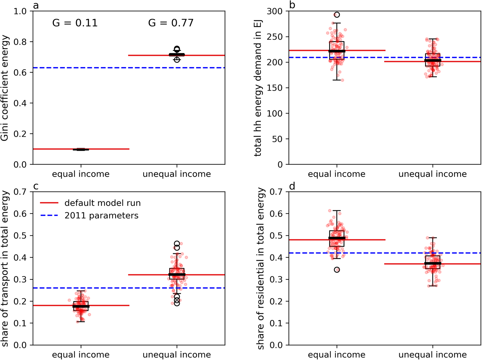
Fig. 7. Monte Carlo simulation results. Panel (a) obviously displays a significant difference between the two income distributions and the resulting energy inequality. Panel (b) depicts the impact on total global household energy demand and the finding that total demand rises in an equal world about ~7% and most likely falls around 3–4% in an unequal world. Panels (c) and (d) depict the impact of redistribution on the sectoral composition of household energy demand, particularly on transport energy and residential energy demand. The differences in panels (c) and (d) are significant based on t-tests and a two-tailed p-value: for instance amounting to p < 0.001 for panel (c). The black lines in the centre of the boxplots display the Monte Carlo simulation median. The red lines show the values attained in the default model run and the dashed blue lines running across the panels represents the parameter estimates for 2011.
4. Discussion and conclusions
The theme redistribution might be quickly associated with political economy. This study, however, treats redistribution rather as a structural transformation than a political one. We can conclude little about political economy from this study. Strong redistributive measures, as for instance the 90% wealth tax on billionaires that Thomas Piketty proposes or universal basic income, naturally require a certain degree of intervention by the state. Redistribution on an international scale requires genuine international cooperation. In principle, however, redistribution is compatible with various forms of political economy, more centralized or more decentralized ones. To this end, we have to refer the reader to other studies that elaborate on contemporary political economy, its shortcomings and ways forward (Creutzig, Reference Creutzig2020; Pirgmaier & Steinberger, Reference Pirgmaier and Steinberger2019; Wiedmann et al., Reference Wiedmann, Steinberger, Lenzen and Keyßer2020). It is also a misconception to associate redistribution only with explicitly redistributional policies. This is not what we have studied. Simulation no. 1 for example is completely agnostic about how lower inequality comes to be. If, let us say, OECD countries would decide to pursue degrowth and the African economy further grows, but there is no direct redistributional link between the two processes, the end result still is a redistribution of global economic wealth.
Exact numbers are to be taken with a large grain of salt and should not be considered empirical data. For example, the model does not adequately represent the number of extremely poor in the world, and rather underestimates it. This is because we used a constant factor to convert a ‘per adult equivalent’ distribution to a ‘per capita’ one. This overlooks the fact that household size in developing countries is often larger than in high-income countries. The results are also in parts dependent on the choice of the distributional model. For instance, varying parameters of a Weibull distribution or of a Pareto distribution shifts the population in different ways as compared to the log-normal model and allocates other quantities of population to specific income levels. However, we tested several such alternative distributions and found that the overall energy demand trends, as a function of the inequality, are stable, even under entirely different income distributions (for details refer to Supplementary Note 5). Another simplification is that the model operates with homogenous energy intensities across the entire distribution. This is clearly not a fully accurate description of reality but it proved useful in answering our questions. The contribution of the model lies in illuminating qualitative characteristics of global income redistribution and its relationship to household energy demand.
Based on our results, marginal and drastic income redistribution prove to be levers for change. This naturally is the case when it comes to inequality. Lower inequality in energy could have manifold benefits, particularly to the people increasing their energy consumption from insufficient levels to sufficient ones. People being lifted out of energy poverty would gain access to a vast range of additional energy services beyond rudimentary nutrition; such as health, residential energy use and necessary mobility. Yet, the ‘energy costs’ of greater equity are small (and may not be significant, as per the simulation in section 3.3). In the simple inequality reduction simulation (section 3.1), the difference between the most equal world (~220 EJ) and the most unequal one (~200 EJ) is 20 EJ which is about 10% of current household energy demand, and ~5% of total global final energy consumption. This is good news for the climate and the feasibility of energy development. It supports previous results demonstrating that climate protection and energy development do not have to be trade-offs, if we allow for diffusion of the right technologies (Wilson et al., Reference Wilson, Grubler, Bento, Healey, de Stercke and Zimm2020) and take sufficiency into account as a mitigation strategy for the affluent (Chakravarty et al., Reference Chakravarty, Chikkatur, Coninck, De, Pacala, Socolow and Tavoni2009; Rao & Min, Reference Rao and Min2018b; Scherer et al., Reference Scherer, Behrens, de Koning, Heijungs, Sprecher and Tukker2018). In addition, if we were to relax the assumption of constant energy intensities, by for example, redistributing to less energy-intensive public spending, the overall energy costs of equity could shrink further.
Despite having built a very simple model with obvious limitations, we show in the floor/ceiling simulation (section 3.2) that by redistributing the existing ‘economic pie’ on the planet, we could lift billions of people out of severe energy poverty without pushing anyone else into it. As little as 1% of the global population could benefit the bottom 40%, with the former retaining yearly incomes above $100,000 PPP and an energy consumption of up to 200 GJ/capita/yr, and the latter all lifted up to at least ~12 GJ/capita/yr. These findings might particularly be relevant to degrowth scholars as they point to a more precise quantification of degrowth: How much does the economy have to degrow? Which levels of income and energy consumption are desirable and feasible? Yet, further specifics, besides household energy levels, of non-growing, degrowing or redistributive economies are beyond the scope of this paper, despite their interest. This ‘transfer’ could also be interpreted as making significant strides towards at least three of the Sustainable Development Goals (SDGs): firstly, ‘#7 Affordable and clean energy for everyone’ (in parts, clean is not guaranteed based on our model), secondly ‘#10 Reduced inequalities’ and thirdly ‘#1 No poverty’. This is not at all obvious considering that global economic growth is often portrayed as something we must rely upon in order to eradicate poverty, even in high-income countries. In all likelihood, the potential of redistribution as a lever for the Agenda 2030 is still underestimated. There is a vast amount of proven synergies between the SDGs (Fuso Nerini et al., Reference Fuso Nerini, Tomei, To, Bisaga, Parikh, Black and Mulugetta2018).
From an energy system point of view, we address a previously understudied relationship. The composition of household energy demand and the degree of income inequality are related. People at different levels of the income spectrum have different energy consumption profiles. In sum, this influences the overall composition of demand. For example, in the simple inequality change scenario (section 3.1), we clearly observe that an unequal world allocates a higher energy share to transport whereas an equal one allocates more to residential energy use. The difference comes mostly from high demand for private vehicles and fuel among a minority elite. Consequently, with increasing income inequality, there is increasing polarization between rich and poor in terms of mobility. We do not distinguish between flying and public transport as they are taken together in one consumption category, which is a constraint due to the underlying consumption surveys. If we would do so, it would further amplify the observed polarization. In fact, the mobility polarization already is a real-world phenomenon. There are now studies that show that the super-rich have disproportionally large carbon footprints due to flying (Gössling, Reference Gössling2019; Otto et al., Reference Otto, Kim, Dubrovsky and Lucht2019) and typical hobbies of super-rich individuals include collecting transport items, such as expensive cars and yachts (Featherstone, Reference Featherstone2014). In contrast, it has been estimated that 80% of people world-wide never have taken a flight (Negroni, Reference Negroni2016). Although somewhat speculative, the result suggests that an equal world might even be more compatible with climate constraints, not less (Hubacek et al., Reference Hubacek, Baiocchi, Feng and Patwardhan2017). Technologies for reducing energy demand in buildings are manifold and often already effective at a low cost (Harvey, Reference Harvey2009), whereas transport is the one sector that is intertwined with the fossil fuel industry. There are of course many efforts to electrify transport on land, in air and on water, but the diffusion of electric cars is projected to remain slow and they are resource-intensive to produce. Electrifying long-distance air transport remains unsolved and water-cargo remains challenging (Davis et al., Reference Davis, Lewis, Shaner, Aggarwal, Arent, Azevedo, Benson, Bradley, Brouwer, Chiang, Clack, Cohen, Doig, Edmonds, Fennell, Field, Hannegan, Hodge, Hoffert and Caldeira2018). A limit to these conclusions is they rest on the assumption that there is no fundamental change to consumer preferences. If income elasticities of demand were to change drastically, as it might happen in the face of profound cultural change, the relationship between inequality and energy demand could exhibit different traits. An example for such profound change is the potential shift away from globalization, including a reversal of the decade long trend of increasing international tourism, towards local forms of production, consumption and leisure.
Obvious continuations of the present study would be to elaborate on the role of specific countries, on policies for redistribution and the acceptance of redistribution of income or energy among the population (as for example studied in Europe; Olivera, Reference Olivera2015). Redistribution within countries might be easier to achieve than redistribution internationally, thus we recommend to further explore redistributive pathways for nations in particular. There are also many technical aspects of this study which future research can build upon. For instance, the granularity and segmentation of consumption categories could have been different. Alternative survey data might provide new opportunities to adjust the model with respect to consumer preferences and elasticities of demand. We purposefully isolated redistribution from other variables for this study, but it might prove useful to integrate income redistribution into larger structural models, such as for instance input–output models. The systemic ramifications of income redistribution deserve further attention.
Supplementary material
The supplementary material for this article can be found at https://doi.org/10.1017/sus.2021.1.
Data
All data and Python code is available on https://github.com/eeyouol.
Acknowledgements
We would like to thank the editors and two anonymous reviewers for their constructive comments.
Author contributions
Y.O., J.K.S., J.M.H. and D.I. conceived and designed the study. Y.O. conducted data gathering and analysis. Y.O., J.K.S., J.M.H. and D.I. wrote the article.
Financial support
Y.O., J.K.S. and J.M.H. are supported by the Leverhulme Trust's Research Leadership Award ‘Living Well Within Limits’ (RL2016-048) project awarded to J.K.S. Y.O. was partly supported through a fee contract by the International Institute for Applied System Sciences (IIASA) in order to explore demand-side concepts, options and policies which could lead to a low energy demand future. D.I. received funding from the UK Research and Innovation (UKRI) Energy Programme under the Centre for Research into Energy Demand Solutions (Engineering and Physical Sciences Research Council (EPSRC) award EP/R035288/1).
Conflict of interest
The authors declare no competing interests.


 Open access