


Introduction
Polarization in many functional materials plays an important role in their technological impact. Properties such as pyroelectricity, piezoelectricity, and ferroelectricity are a direct consequence of changes in polarization caused by a thermal, mechanical, or electrical stimulus, enabling a wide range of functional devices including sensors, actuators, modulators, nonvolatile memories, and capacitive devices. However, enhancing the polarization response of materials through crystal chemical or microstructural design remains an important area of research, and accurate measurements at the micro- and nanoscale are required to gain more insights into local variations in polarization and switching mechanisms.
Polarization, as described by the modern theory of polarization (Resta & Vanderbilt, Reference Resta and Vanderbilt2007), is a periodic lattice rather than a vector, and thus, only the difference of polarization between two states can be uniquely defined. This theory divides polarization into two main components, the electronic and ionic part, as described by equation (1), where P is the total polarization, e is the electronic charge, the integral represents the Berry phase, which is summed over n valence bands, Ω is the unit cell volume, Z ion is the net positive charge of the nucleus plus core electrons, r is the atomic position, and s the species.
 $$P = \displaystyle{e \over {{( {2\pi } ) }^3}}{\mathop{\rm Im}\nolimits} \mathop \sum \limits_n \int {dk\; {\langle} u_{nk}\vert {\nabla_k} \vert u_{nk}} {\rangle} + \displaystyle{e \over \Omega }\mathop \sum \limits_s Z_s^{{\rm ion}} r_s.$$
By determining the location of all atomic positions, the ionic contribution to the local polarization is, in principle, easily calculated from equation (1). Nevertheless, to compute the total polarization, the electronic component needs to be included. Both contributions can be simultaneously calculated from the atomic displacements using the Born effective charges (obtained by ab initio calculation) according to the following equation:
 $$\Delta P_\beta = \displaystyle{e \over \Omega }\;\mathop \sum \limits_s Z_{s, \alpha \beta }^\ast \Delta r_{s, \alpha }.$$
Here Pβ is the total polarization in the direction β, e is the electronic charge, Ω is the unit cell volume, Z* is the Born effective charge for atom s, Δr is the atomic displacement between the two states in the direction α (i.e., paraelectric to ferroelectric states), and α and β being Cartesian coordinates.
Polarization measurements are usually based on macroscopic measurements using polarization–electric field loops based on the Sawyer–Tower circuit (Sawyer & Tower, Reference Sawyer and Tower1930) or local spatially resolved optical measurements such as Second Harmonic Generation (Denev et al., Reference Denev, Lummen, Barnes, Kumar and Gopalan2011) at the micrometer scale. Electron microscopy-based techniques, on the other hand, have been pursued to measure local polarization at the sub-nanometer scale for imaging nanopolar regions of relaxor ferroelectrics, ferroelectric domains walls, and polar vortices (Jia et al., Reference Jia, Nagarajan, He, Houben, Zhao, Ramesh, Urban and Waser2007; Nelson et al., Reference Nelson, Winchester, Zhang, Kim, Melville, Adamo, Folkman, Baek, Eom, Schlom, Chen and Pan2011; Estandía et al., Reference Estandía, Sánchez, Chisholm and Gázquez2019; Moore et al., Reference Moore, Conroy and Bangert2020). To achieve local polarization measurements, researchers have employed techniques such as Fourier masking high-resolution transmission electron microscopy (TEM) images (Moore et al., Reference Moore, Conroy and Bangert2020), position-averaged convergent beam electron diffraction (Lebeau et al., Reference Lebeau, D'Alfonso, Wright, Allen and Stemmer2011), charge distribution using 4D-STEM and differential phase contrast (Gao et al., Reference Gao, Addiego, Wang, Yan, Hou, Ji, Heikes, Zhang, Li, Huyan, Blum, Aoki, Nie, Schlom, Wu and Pan2019), and atomically resolved scanning TEM (STEM) images to identify the relative shift of sublattices (Moore et al., Reference Moore, Bangert and Conroy2021) or the displacement of the atomic columns with respect to a centrosymmetric structure (Abrahams et al., Reference Abrahams, Kurtz and Jamieson1968; Jia et al., Reference Jia, Nagarajan, He, Houben, Zhao, Ramesh, Urban and Waser2007; Zhu et al., Reference Zhu, Chen, Tian and Chen2017; Estandía et al., Reference Estandía, Sánchez, Chisholm and Gázquez2019; Sun et al., Reference Sun, Abid, Tan, Ren, Li, Li, Chen, Li, Zhang, Zhong, Wang, Liao, Liu, Bai, Zhou, Yu and Gao2019; Moore et al., Reference Moore, Conroy and Bangert2020). The later technique directly applies equation (2), obtaining quantitative results, which strongly relies on the accurate determination of the atomic-column positions. The selection of the imaging modality, microscope parameters, and sample parameters (e.g., thickness) can significantly affect the measured atomic-column locations (Gao et al., Reference Gao, Kumamoto, Ishikawa, Lugg, Shibata and Ikuhara2018) and, in turn, affect the measured polarization. Thus, to understand the accuracy of projected polarization measurements from atomic-resolution STEM images, a systematic study of the effect of these experimental parameters is necessary.
To measure the atomic-column positions, researchers have employed different techniques, including phase-contrast, high-angle annular dark-filed (HAADF), annular bright-field (ABF), and integrated differential phase-contrast images (iDPC) (Lazic et al., Reference Lazic, Bosch and Lazar2016). Among these techniques, iDPC has attracted significant interest due to its capacity to simultaneously image light and heavy atoms, particularly important for the study of numerous important materials such as metal oxides and nitrides. iDPC belongs to a family of techniques known as differential phase contrast (DPC) originally proposed by Dekkers and de Lang (Dekkers & de Lang, Reference Dekkers and de Lang1974) and later extended by Rose (Rose, Reference Rose1976) and Waddell and Chapman (Waddell & Chapman, Reference Waddell and Chapman1979). DPC family of techniques (iDPC, DPC, and dDPC) is an approximation of the center of mass techniques (iCoM, CoM, and dCoM), which can be linearly related to the phase, the gradient of the phase, and the Laplacian of the phase of the sample transmission function, respectively.
In this work, we compare different STEM imaging modalities for their ability to provide accurate measurements of polarization in materials. We aim to address the following questions associated with calculating polarization from STEM images including (i) which imaging mode provides the highest accuracy for measuring polarization, (ii) what errors are introduced from multiple atomic species within an atom column, and (iii) the implications of chemical/structural heterogeneities along the beam projection. Our approach is to employ model structures, which serve as ground-truth, and to simulate STEM images under varying sample and microscope parameters. Multislice image simulations are used to evaluate systematically the effect of microscope and sample parameters (such as probe size, converge angle, thickness, and defocus) on the measurement of the projected polarization. We demonstrate that dDPC significantly reduces the error for the calculation of the polarization compared with iDPC and ABF.
Methods
Two different structures are used to evaluate the ability of STEM to determine the local polarization. First, a pure ZnO Wurtzite phase with space group P63mc (Jain et al., Reference Jain, Ong, Hautier, Chen, Richards, Dacek, Cholia, Gunter, Skinner, Ceder and Persson2013) is used as a simple approach to illustrate the calculation of projected spontaneous polarization from STEM images when compared to a centrosymmetric reference phase, such as a h-BN like ZnO structure (Tusche et al., Reference Tusche, Meyerheim and Kirschner2007). In this system, there is no overlapping of the cation and anion sublattices along the [110] direction, making it a relatively simple case.
As the second case of study, a very common perovskite structure for nonlinear dielectric materials is selected. This material, PbMg1/3Nb2/3O3 (PMN), provides an ideal model to consider complex effects on the projected polarization, such as (i) disordered cation composition, (ii) large contrast between the atomic-columns (e.g., Pb and O), (iii) overlapping of projected atomic sublattices in all low-order zone axes, and (iv) significant difference between the Born effective charges and formal valance charges.
ZnO Wurtzite Structure
The ZnO wurtzite structure (Jain et al., Reference Jain, Ong, Hautier, Chen, Richards, Dacek, Cholia, Gunter, Skinner, Ceder and Persson2013) is selected as the atomic model from which we calculate the “ground-truth” polarization value. We simulate and acquire experimental images on the [110] zone axis, which is perpendicular to the polar axis in ZnO. Hence, in this case, the projected polarization is equivalent to the actual spontaneous polarzation.
Multislice computer simulations are used to simulate HAADF, ABF, and DPC images (from a quadrant detector) using the Dr. Probe V1.9 software package (Barthel, Reference Barthel2018). Simulations for the ZnO structure are carried out using the frozen-phonon method with 900 configurational variants to ensure convergence of each atomic position to its average position from the atomic model within a 1 pm error. Images are simulated at 200 keV and 1 μm of spherical aberration, while varying the probe size, defocus values, sample thickness, and crystal tilt. The potential discretization is set at 144 pixels × 144 pixels (approximately 0.004 nm/pixel), and the thickness of the slices is 0.164 nm (one atomic layer). Convolution with a finite source size varying from 60 to 90 pm is carried out. The resulting probe size is tabulated in Supplementary Table S1.
Calculation of the total polarization from a ZnO reference model
ZnO has a spontaneous polarization along the [001] direction, which can be calculated with respect to a centrosymmetric reference phase, such as a h-BN-like ZnO structure (Tusche et al., Reference Tusche, Meyerheim and Kirschner2007) using equation (2). Based on this centrosymmetric phase, the polarization is simplified to  $\Delta P = {{2eZ_{\rm O}^\ast \Delta u} / \Omega }$, where e is the electronic charge, $Z_{\rm O}^\ast$ is the oxygen Born effective charges, Δu the displacement of oxygen relative to zinc along the [001] direction, and Ω the unit cell volume. The resulting value (0.886 C/m2) is used as ground-truth to compare with the values obtained from simulated and experimental STEM images.
PbMg1/3Nb2/3O3 Perovskite Structure
A disordered PMN structure of 6 × 6 × 6 unit cells generated by special quasi-random structures (SQS) (Kumar et al., Reference Kumar, Baker, Bowes, Cabral, Zhang, Dickey, Irving and LeBeau2021) is used as a “ground-truth” model to calculate the polarization and perform multislice computer simulations.
Frozen-phonon configurations for multislice simulations require a very large number of variants per slice (>900) in order to converge the position of each atom within less than 1 pm error from the model, in this case, demanding several weeks for each simulation. Combined with the large number of simulations (>25) used in this study, it is thus to use this approach impractical from a computation point of view. Thus, an adsorptive potential approach is used for all simulations of the PMN supercell.
This is justified by noting that, while thermal diffuse scattering (TDS) is better simulated using the frozen-phonon model, for DPC and ABF imaging the TDS contribution is small (Findlay et al., Reference Findlay, Shibata, Sawada, Okunishi, Kondo and Ikuhara2010; Müller-Caspary et al., Reference Müller-Caspary, Krause, Grieb, Löffler, Schowalter, Béché, Galioit, Marquardt, Zweck, Schattschneider, Verbeeck and Rosenauer2017). On the other hand, HAADF is dominated by TDS; however, it has been demonstrated that the atomic position accuracy using adsorptive potentials is similar to that obtained by frozen phonons, with differences of around 1 pm (Alania et al., Reference Alania, Lobato and Van Aert2018). This error is smaller than the smallest standard deviation of the atomic displacements in the model (6 pm).
Simulations are carried out with 200 keV electrons and 1 μm of spherical aberration while varying the probe size, convergence angle, defocus, sample thickness, and tilt. The potential discretization is set at 600 pixels × 600 pixels (0.004 nm/pixel approximately), and the thickness of the slices is 0.176 nm (one atomic layer). Convolution with a finite source size varying from 60 to 90 pm is carried out. The resulting probe size is tabulated in Supplementary Table S1.
It is important to note that the 6 × 6 × 6 DFT supercell is tiled along the z-direction to change the thickness of the model. While this may not accurately represent the polarization likely to be measured from a real PMN sample, this procedure does allow us to measure the effect of the thickness and defocus on the determination of polarization from STEM images by comparing values measured from a simulated image with the true values obtained from the underlying structure.
Calculation of the total polarization from the PMN reference model
The total polarization per unit cell of the DFT-based PMN model is calculated using equation (2) and the Born effective charges reported by Prosandeev et al. (Reference Prosandeev, Cockayne, Burton, Kamba, Petzelt, Yuzyuk, Katiyar and Vakhrushev2004). Atomic displacements are calculated with respect to a centrosymmetric perovskite structure PMN, with the space group Pm3̅m and a cell parameter a = 0.4105 nm. A 6 × 6 × 6 unit cell cube with 3D polarization vectors are obtained from the atomic model, where the x-axis points to the [100] direction, y-axis to the [010] direction, and z-axis along [001], as shown in Figure 1a.

Fig. 1. (a) 3D polarization for a 6 × 6 × 6 unit cell atomic model. (b) 3D representation of a unit cell with the respective atom occupancies. (c) 2D-projected unit cell with the respective atomic column occupancies.
Taking into consideration that the STEM images only offer projected atomic-column positions and that the oxygen and B-cation sublattices overlap along the [001] direction, we first explore the implications of these projection effects from the model structure itself. We begin by comparing the 2D projection of the 3D polarization with a 2D polarization calculated after first projecting the 3D structure into atomic-column positions like those obtained in a STEM image.
3D ground-truth: The polarization is calculated from the model structure using equation (2) and the Born effective changes of  $Z_{{\rm Pb}}^\ast{ = } 4$, $Z_{{\rm Mg}}^\ast{ = } 2.6$, $Z_{{\rm Nb}}^\ast{ = } 7.4$, $Z_{{\rm O}\parallel }^\ast{ = }{-}4.8$, and $Z_{{\rm O\ + \ }}^\ast{ = }{-}2.5$, where the subscripts ∥ and + denote the directions of the oxygen displacement–vector components parallel and perpendicular to the Mg/Nb–O bond, respectively. The Born effective charge is multiplied by the occupancy of each atom in the unit cell, as shown in Figure 1b. The displacements are divided into components x, y, and z, and the polarization P is calculated as Px, Py, and Pz for the x, y, and z components pointing along directions [100], [010], and [001], respectively. Then, the projected polarization is obtained as an average value of all unit cells along the beam direction as shown in Figure 1a.
2D projected polarization: By calculating the 2D polarization from the structure projected into a 2D lattice, we show the best-case scenario for measuring the polarization from a STEM image. In this approach, the atomic positions are averaged along the beam direction before calculating the polarization. Due to our choice of unit cell (Fig. 1c), each projected Pb position contributes ¼ to the total Pb charge in the unit cell, and the four separated oxygen columns each contribute ½. However, the superposition of Mg/Nb and central oxygen columns in STEM images prevent separately resolving them. It is assumed that the position of the Mg/Nb/O column is completely dominated by the B-site cations. In the 2D projection calculation, only the Mg/Nb positions are averaged to find the B-site column location (ignoring the central oxygen atoms). The charge of the Mg/Nb columns is calculated from the stoichiometry of the system as  $( {1/3\ast Z_{{\rm Mg}}^\ast{ + } 2/3Z_{{\rm Nb}}^\ast } )$, with no effort made to account for differences in column compositions. The movement of the central oxygen is assumed to equal the average projected displacement of the other four oxygen columns in the cell. The assigned Born effective charge for the central oxygen is always $Z_{{\rm O\ + \ }}^\ast$ because its projected displacements are perpendicular to the near-neighbor B-site bonds. This same charge-weighting procedure is used to calculate the polarization from the simulated STEM images.
In order to determine the deviation of the 2D-projected methodology from the ground-truth 3D method, two figures of merits are used, namely the correlation coefficient (R 2) and root-mean-square deviation (RMSD) between ground-truth and the projected polarization (Fig. 2). Only small deviations are observed for each component, which supports the assumption of displacement correlation between the central oxygen and the octahedral corners. Note that the best approach to treating atomic columns containing mixed species may be particular to a structure or composition and that obtaining a good approximation of the polarization depends on validating this decision.

Fig. 2. Linear regression between ground-truth polarization and the polarization calculated after projection for (a) x-component and (b) y-component, and (c) colour-map representation of the polarization where the arrows represent the normalized magnitude and direction of the polarization for the ground-truth (blue) and after projection (black).
Experimental ZnO Image Acquisition
DPC-STEM images are acquired in a ThermoFisher Titan–Themis operated at 200 kV using a four-segment annular detector (DF4), a probe convergence angle of 25 mrads, and a camera length that resulted in acceptance angles between 11 and 43 mrads. A set of 30 frames are collected using fast dwell time (200 ns) to avoid significant drift that can cause distortions in the images. The frames are later registered using cross-correlation and integrated to improve the signal-to-noise ratio. Final error in the cell distortion is calculated using a reference ZnO lattice from a crystallographic file, obtaining values of 0.8% and 0.0076 rads for the scaling and shear components, respectively. The sample thickness is estimated using a position-averaged convergent beam electron diffraction (PACBED) pattern obtained from the region of interest and compared with simulated PACBED images.
Image Analysis and Quantification
Simulated and experimental iDPC and dDPC images are calculated according to the reference (Lazic et al., Reference Lazic, Bosch and Lazar2016). Briefly, iDPC images are calculated using the expression shown in equation (3), where I DPC(rp) can be decomposed into x and y components, corresponding to the difference between opposite segments in the detector, multiplied by the size of the bright-field disk and the constant  $\pi /2\sqrt 2$.
dDPC images are calculated as the differentiated DPC signal [equation (4)], which is equivalent to the Laplacian of the iDPC signal.
 $${\cal F}{ {I^{{\rm iDPC}}( {\overrightarrow {r_p} } ) } } ( {\overrightarrow {k_p} } ) = \displaystyle{{{\vec{k}}_p{\cal F}{ {I^{{\rm DPC}}( {\overrightarrow {r_p} } ) } } ( {\overrightarrow {k_p} } ) } \over {2\pi ik_p^2 }},$$
 $$I^{{\rm dDPC}} = \nabla ^2I^{{\rm iDPC}}( {{\vec{r}}_p} ). $$
The positions of the atomic columns are initially approximated to a reference crystallographic file and then refined using Atomap (Nord et al., Reference Nord, Vullum, MacLaren, Tybell and Holmestad2017) or the SingleOrigin Python module described in Funni et al. (Reference Funni, Yang, Cabral, Ophus, Chen and Dickey2021) and available here (https://doi.org/10.1184/R1/14318765).
For ZnO, due to the proximity of the Zn- and O-projected columns (0.114 nm), these “dumbbell” intensity distributions are fitted with two Gaussians simultaneously, ensuring that the effect of the nearby atomic column is taken into consideration. Due to the sufficiently large column separations in PMN; on the other hand, each atom column position is fitted individually. The refined positions are separated into sublattices by elements (e.g., Zn and O; Pb, Mg/Nb, and O). Note, however, that the Mg/Nb columns in the projected PMN structure have overlapping O atoms.
Three different image types are used to locate the position of the atomic columns: (i) a combination of HAADF and ABF, (ii) iDPC, and (iii) dDPC. The first method uses the combination of HAADF and ABF because the higher signal-to-noise ratio of HAADF helps to improve the determination of the heavy-element columns, while ABF is only used to locate the lighter elements undetected by HAADF (Gao et al., Reference Gao, Kumamoto, Ishikawa, Lugg, Shibata and Ikuhara2018). iDPC and dDPC signals, on the other hand, are used to determine the position of both heavy and light elements simultaneously.
Gaussian Process Regression
Due to the computational demand on the PMN model for each image simulation, a 2D Gaussian process regression was used to estimate the residuals of polarization as a function of thickness and defocus from a small set of simulated combinations. The Gaussian process models all the observations using a multivariate normal distribution with a radial-basis function as a covariance. The regression is carried out by sci-kit-learn package in Python (Pedregosa et al., Reference Pedregosa, Varoquaux, Gramfort, Michel, Thirion, Grisel, Blondel, Prettenhofer, Weiss, Dubourg, Vanderplas, Passos, Cournapeau, Brucher, Perrot and Duchesnay2011) using 17 thickness–defocus pairs maintaining all the other parameters in the microscope constant.
Results and Discussion
First Case Study: ZnO Wurtzite Structure
Effect of microscope parameters on ZnO spontaneous polarization measurement
Figure 3 shows simulations from ABF, iDPC, and dDPC at different source sizes, with the respective intensity profiles for one of the Zn–O dumbbell atomic-column pairs (Fig. 3b). The vertical dashed lines in the profiles schematize the true location of the atomic columns obtained from the model. Notice that HAADF is not included due to the lack of oxygen signal. The profiles exhibit an overlap in the Zn and O atomic-column intensities when observed along the [110] direction. Such overlap hinders accurately locating the atomic columns in some image modalities, such as ABF and iDPC, where no intensity minimum can be observed between the two atomic columns for source sizes higher than 60 pm. In contrast, dDPC shows a clear separation of the columns, with an intensity drop between columns of 8–50% compared to the oxygen maximum intensity, facilitating an unequivocal fitting of two Gaussian functions.

Fig. 3. (a) ABF, iDPC, and dDPC STEM-simulated images at different source sizes and (b) intensity profiles across the Zn–O dumbbells as exemplified by the red arrow in (a). (b) ABF intensity was inverted (iABF) to directly compare with iDPC and dDPC and (c) movement of the intensity maximum from the true position for the Zn and O atomic column as a function of the source size for ABF, iDPC, and dDPC.
To determine the effect of the overlapping Zn–O atomic-column intensity distributions, we calculate the measured displacement from the ground-truth position for the three different image modes, as shown in Figure 5c. Larger deviations for the oxygen atomic-column position are observed for ABF and iDCP images compared to dDPC. In addition, dDPC images show insignificant dependence on the probe size.
In order to determine the effect of thicknesses and defocus conditions to improve the location of the atomic columns, multislice computer simulations are performed for ABF, iDPC, and dDPC convolved with an 80 pm source size. Figure 4a shows the thickness–defocus map for ABF, revealing significant contrast dependence with defocus, to a point in which the oxygen atomic columns reverse contrast. Figures 4b and 4c, on the other hand, show a most robust contrast behavior for iDPC and dDPC images, where no contrast inversion is observed. However, independent of the thickness and defocus values, iDPC does not separate the two atomic columns, leading to larger errors when locating the atomic-column positions, as previously shown.
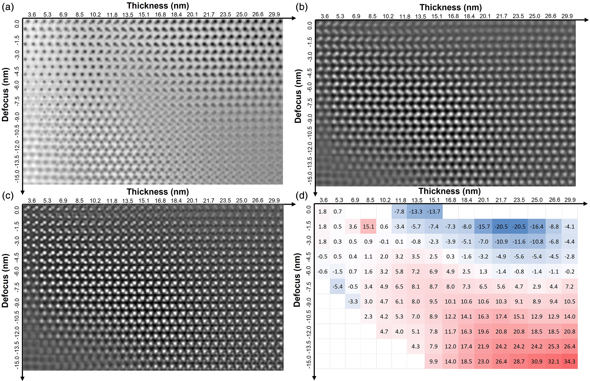
Fig. 4. Multislice computer simulation of defocus–thickness map for a single ZnO unit cell along the [110] orientation for (a) ABF, (b) iDPC, (c) dDPC, and (d) percent error of the measured polarization from dDPC compared to the value calculated from the structure. Positive values in the relative errors represent the overestimation of the polarization, while negative values represent the underestimation of the polarization.
Thus, considering that Zn–O dumbbell are better resolved with dDPC, the ZnO polarization was calculated from the dDPC thickness–defocus map and compared with the ground-truth value calculated from the model. Figure 4d shows the relative error of polarization as a function of thickness and defocus. Positive values in the relative errors represent the overestimation of the polarization, while negative values represent the underestimation of the polarization. The results show accurate polarization values calculated from dDPC images (within 8% of the ground-truth value) over a large range of thickness (<20 nm) and defocus (>−6 nm) values. In the case of large defocus values, the polarization tends to be overestimated with a noticeable tendency to increase as the defocus is increased. However, no clear tendency is observed for the estimation of the polarization as a function of thickness (see Supplementary Material). Special care needs to be placed for thicker samples, where the non-symmetric contrast transfer function of the segmented detector significantly affects the image (Lazic et al., Reference Lazic, Bosch and Lazar2016) and introduces a dependence on the relative sample-to-detector orientation. This limitation may be overcome using fast pixelated detectors (Jannis et al., Reference Jannis, Hofer, Gao, Xie, Béché, Pennycook and Verbeeck2022) to perform 4D-STEM acquisitions using integrated and differentiated center of mass (iCOM and dCOM). Nonetheless, segmented detectors are currently more widely available and have the advantages of faster post-processing and lower data storage demands relative to 4D-STEM.
We also consider the effect of dose on the accuracy of the atomic column location measurements that underly the polarization calculation. In general, iDPC imaging is robust to noise due to the integration process used to calculate it. On the other hand, the derivative necessary to calculate the dDPC image tends to increase the noise level, thereby making it more sensitive to shot noise. For simulated images of [110] ZnO, with the close spacing of its Zn–O dumbbells, doses less than 105 e/Å2 result in a rapidly increasing position measurement error, especially for the oxygen columns (see Supplementary Material). iDPC images show a much less pronounced degradation in the position errors; however, the errors are much larger than those found from dDPC images at doses of 105 e/Å2 and higher. The magnitude of the errors measured from iDPC images are likely unacceptable for many purposes. We point out that a 105 e/Å2 dose is obtained using a 32 pA probe, 5 µs dwell time, and 10 pm step size, relatively standard imaging conditions. At these typically used doses, both the precision and accuracy of atom column measurements from ZnO dDPC images are within 5 pm. The effect of noise on the measurement of atomic column positions is always dependent on the structure and orientation observed, with closely spaced columns presenting the greatest challenge. For beam-sensitive materials requiring lower doses, simulations should be used to verify the level of accuracy expected for the polarization measurement.
In order to determine the effect of the specimen tilt on the measured polarization, images were simulated for tilts along [β 1 0] and [1 β 0] from the [110] zone axis, with β = 0, 1, 2, 4, and 8 mrads. Figure 5 shows the relative error of the polarization calculated between the atomic model and the dDPC images. Although a clear tendency to increase the error of the measured polarization is observed as a function of tilt angles, for small sample tilts (≤4 mrads), the value of the polarization is generally within 8% relative error from ground-truth. Tilts higher than 4 mrads become evident during acquisition, and thus, mis-tilt of the sample must be minimized to accurately quantify the polarization.

Fig. 5. Relative error measurements of polarization calculated between the atomic model and the dDPC images (a) for tilts along [β 1 0] and (b) for tilts along [1 β 0] from the [110] zone axis. Positive values in the relative errors represent the overestimation of the polarization, while negative values represent the underestimation of the polarization.
To validate the simulation results, ZnO experimental images are obtained. Figure 6 shows a ZnO region of approximately 6.6 nm in thickness imaged by iDPC and dDPC. The polarization is calculated for each unit cell in the dDPC images using the same procedures as for simulated images. The results reveal an averaged polarization of 0.898 ± 0.044 C/m2 within 1.4% relative error compared to the theoretical value obtained from the unit cell model. The polarization was also calculated from 2,500 unit cells from a collection of images acquired in regions with a small variation of the thickness (6–14 nm) obtaining an average polarization of 0.867 ± 0.072 C/m2, which corresponds to a 2.1% relative error compared to the theoretical value. It is worth noting that a small tilt along the [β 1 0] from the [110] zone axis (<6 mrad) is observed in the experimental PACBED, while no tilt is detected along the [1 β 0] from the [110] zone axis. Thus, the tilt contribution for the calculation of the polarization is expected to be below 1% of relative error, as shown in Figure 5.
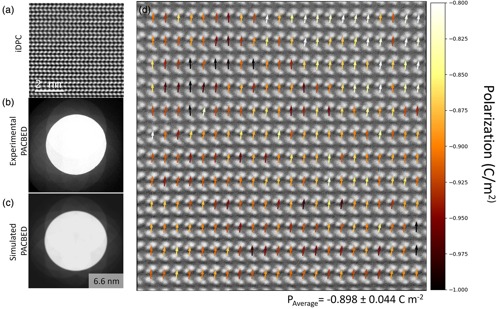
Fig. 6. (a) iDPC experimental image of the ZnO single crystal oriented along the [110] direction, (b) experimental PACBED of the region shown in (a,c) simulated PACBED for a ZnO oriented along the [110] direction with 6.6 nm of thickness, and (d) dDPC image overlapped with arrows representing the polarization calculated from each unit cell.
Second Case of Study: PbMg1/3Nb2/3O3 Perovskite Structure
Effect of microscope parameters on spontaneous polarization determination
Effect of probe size
The probe size in STEM images is one of the parameters that limits the resolution and, therefore, has a significant effect on the determination of the position of the atomic columns. The final probe size is the combination of the finite source size at the object plane set in terms of a full-width-at-half-maximum height (FWHM) of a Gaussian distribution and the coherent probe calculated based on the microscope parameters.
Figure 7 shows the evolution of the simulated ABF, HAADF, iDPC, and dDPC images of the PMN model structure as a function of the probe size. Although almost visually unnoticeable, variations in the probe size have a significant impact on the determination of the polarization. The effect of increasing the source size is mainly to blur the atomic-columns, which increases the intensity overlap of neighboring columns, influencing the accuracy of Gaussian fitting.

Fig. 7. HAADF, ABF, iDPC, and dDPC multislice computer-simulated images of the 6 × 6 × 6 PbMg1/3Nb2/3O3 model along the [001] orientation with different source size convolution.
A comparison between the ground-truth and the polarization calculated from STEM images shows a monotonic increase in the residuals as the probe size increases for HAADF–ABF and iDPC, as well as a decrease in the R 2 of the linear fits, as shown in Figure 8. However, determining the polarization from the dDPC image is nearly invariant to probe size, displaying lower residuals and higher linearity compared with iDPC and HAADF–ABF images. Such results can be explained by the mathematical formulation of dDPC images, where the Laplacian of the iDPC signal is obtained, which highlights regions of rapid intensity change in the image, narrowing the location of the central position of the atomic-columns, and thus, decreasing the overlap between the neighboring columns and allowing a better fitting.

Fig. 8. The RMSD between the ground-truth and the polarization calculated from the simulated images as a function of source size for (a) x-component and (b) y-component. R 2 between the ground-truth and the polarization calculated from the simulated images as a function of source size for (c) x-component and (d) y-component.
To visualize the differences between HAADF–ABF, iDPC, and dDPC, the polarization per projected unit cell is plotted in Figure 9. For comparison, light blue arrows indicate the polarization calculated from the atomic model, while the black arrows show the polarization calculated using the STEM images. The color of each pixel indicates the magnitude of the polarization, while the arrows indicate the direction and the normalized magnitude of the polarization. It is worth noting that only small deviations in the magnitude and the direction are observed for all the image modes, with overestimation of the polarization for iDPC and HAADF–ABF modes, as evidenced by the residuals in these techniques.

Fig. 9. Color-map representation of the polarization per projected unit cell, where the arrows represent the normalized magnitude and direction of the polarization for the ground-truth (blue) and calculated by the STEM image (black): (a) HAADF + ABF, (b) iDPC, and (c) dDPC.
Convergence angle
Tuning the probe size in real experiments is accomplished indirectly by tuning the convergence angle (α), changing the probe current, and correcting spherical aberrations. By increasing the convergence angle, the distortions of the electron wavefront caused by diffraction of the electrons are limited, reducing the probe size. However, the effects of spherical and chromatic aberrations are increased. As a result, it is relevant to determine the effect of α (for give aberrations) on the calculation of the polarization. For that, we consider α from 15 to 30 mrads, a low spherical aberration (1 μm) and the final images are blurred using a Gaussian distribution, making a conservative estimative for the source size of 80 pm. Again, a comparison between HAADF–ABF, iDPC, and dDPC images is carried out to determine the method that provides the most accurate calculation of the polarization relative to ground-truth.
Figure 10a shows the simulated ABF, HAADF, iDPC, and dDPC images as a function of α from 15 to 30 mrads. As expected, with increasing convergence angle, a better definition of the atomic columns is obtained at low thickness. This produces lower residuals in the calculation of the polarization, making the absolute value of the residual drop below 0.1 C/m2 in all the images, as shown in Figures 10b and 10c. Yet, dDPC images show the lowest residuals and highest R 2.

Fig. 10. HAADF, ABF, iDPC, and dDPC multislice computer-simulated images of a 6 × 6 × 6 PbMg1/3Nb2/3O3 model along the [001] orientation at different convergence angles. The RMSD between the ground-truth and the polarization calculated from the simulated images as a function of convergence angles for (a) x-component and (b) y-component. R 2 between the ground-truth and the polarization calculated from the simulated images as a function of convergence angles for (c) x-component and (d) y-component.
Effect of thickness and defocus
Thickness and defocus may have a significant impact on the calculation of the polarization since three of the imaging modes considered (ABF, iDPC, and dDPC) collect electrons within the bright disk region, which is sensitive to phase changes. HAADF, on the other hand, is formed by incoherently scattered electrons, and therefore, the effect of thickness and defocus in the contrast of the atomic columns is less relevant.
To elucidate the effect of these parameters, a series of STEM images for ABF, iDPC, and dDCP are simulated. Figure 11 shows the evolution of a selected unit cell from the model as a function of thickness and defocus. Clearly, ABF, iDPC, and dDPC are dependent on both parameters but with dissimilar behavior. Small changes in the defocus (2 nm) can lead to the oxygen atomic-columns being indistinguishable from the background in ABF, hindering the location of the atomic-column and thus giving rise to a large difference in the calculated polarization when compared with the ground-truth model. For thin samples, defocus can also induce inversions of contrast of O atomic columns, impeding the proper quantification of their positions. Nonetheless, as the model increases in thickness, more contrast is observed, and easier determination of the oxygen atomic columns at zero defocus can be obtained. The contrast variation is likely to be sample dependent, hence, decreasing the robustness of the technique.

Fig. 11. Multislice computer simulation of the defocus–thickness map of a single-unit cell of the PbMg1/3Nb2/3O3 model along the [001] orientation for (a) ABF, (b) iDPC, (c) dDPC, and (d) Gaussian process regression for the RMSD of polarization using 17 thickness–defocus combinations (red dots) for dDPC images.
Differential phase-contrast images, on the other hand, do not show an inversion of contrast as a function of the thickness or defocus, making them more robust for the location of heavy and light elements. Defocus values different than zero are required to obtain sharp images as the model becomes thicker. The optimum defocus is reliably found to be approximately half the thickness of the model, as previously reported to be the optimum imaging condition (Addiego et al., Reference Addiego, Gao and Pan2020).
Residuals between the polarization measured from dDPC images and the ground-truth from the atomic models are calculated at different defocus–thickness pairs to better elucidate the effect of these parameters on the polarization measurement. For the ZnO structure, a full space of defocus versus thickness pairs was simulated. However, the size of the PMN model precluded simulating the whole space in a reasonable amount of time. Hence, a Gaussian process is used to interpolate a sparce grid of simulation results, as described in the section “Gaussian Process Regression”. The residuals are obtained from 17 different thickness–defocus pairs, as shown in red in Figure 11d. Figure 11d shows the results of the Gaussian process for the residuals. Values closer to zero indicate lower errors between the STEM images and the ground-truth atomic model, showing good agreement with the simulated images in Figure 11c. It is worth noting that regions with very high residuals are not desired and thus were less explored during the Gaussian process. As expected, better resolved images produce a more accurate determination of the polarization, which occurs for DPC imaging when the probe is focused in the middle of the sample, or in a slight under-focus condition. This behavior agrees with results reported by Addiego et al. (Reference Addiego, Gao and Pan2020), who demonstrate that this condition allows a good approximation of the projected electric field calculated from DPC images for thick samples, which, in turn, is expected to correspond to the best conditions to determine the projected potential (iDPC) and projected charge distribution (dDPC).
It has been previously demonstrated that mis-tilt of the sample with respect to the zone-axis orientation can produce artificial displacement of the atomic columns in perovskite structures (Gao et al., Reference Gao, Kumamoto, Ishikawa, Lugg, Shibata and Ikuhara2018). Thus, to quantify the effect of sample tilts on the measured polarization, the PMN model was tilted along [0 β 1] direction from the [001] zone axis with β = 0, 1, 2, 4, and 8 mrads. Figure 12 shows the effect of sample tilt on the RMSD along [100] and [010] directions, x-component, and y-component, respectively. The results indicate a significant effect of mis-tilt on the calculated polarization, increasing the RMSD as a function of tilt angles. Gao et al. (Reference Gao, Kumamoto, Ishikawa, Lugg, Shibata and Ikuhara2018) have demonstrated that no significant artificial displacement is observed between the cation columns in STO, explained by the similar dechannelling of Sr and TiO atomic columns in an ADF image mode. However, a large artificial relative displacement between the anion and cation sublattices was reported as a result of sample mis-tilt. This produces artificial relative displacement between the cation and anion sublattices, which directly correlates with the error in the polarization. Such error is amplified for thicker samples at tilts higher than 4 mrads, and hence, accuracy of the polarization measurement relies on the proper characterization of the specimen tilt. In fact, experimental tilt maps may be used to separate the tilt effect from the actual polarization via simulation.

Fig. 12. The RMSD between the ground-truth and the polarization calculated from dDPC-simulated images as a function sample tilts along the [0 β 1] direction from the [001] zone axis: (a) x-component and (b) y-component.
Conclusions
We demonstrate the ability to accurately measure local spontaneous polarization via STEM under particular sample, microscope conditions, and imaging modalities. dDPC imaging shows a significant improved accuracy for measuring local spontaneous polarization of materials in comparison to HAADF + ABF and iDCP imaging modalities. This is attributed to the fact that a Laplacian operator is used to calculate the dDPC signal from the iDPC images due to the relation between the projected charge distribution (dDPC) and the atomic potential (iDPC). This operation narrows the width of atomic-column intensity distributions, improving location determination and translating into more accurate atomic-column locations and thus polarization measurements. With careful understanding of the optimal sample and microscope conditions, it is possible to measure local polarization on an absolute scale by STEM, bringing us closer to a better understanding of the mechanisms in which polarization states can be engineered.
Supplementary material
To view supplementary material for this article, please visit https://doi.org/10.1017/S1431927622012429.
Acknowledgments
The authors thank Dr Jonathon N. Baker and Prof. Dr Douglas L. Irving for providing the PbMg1/3Nb2/3O3 atomic models from Kumar et al. (Reference Kumar, Baker, Bowes, Cabral, Zhang, Dickey, Irving and LeBeau2021). The authors acknowledge use of the Materials Characterization Facility at Carnegie Mellon University supported by grant MCF-677785.
Conflict of interest
The authors declare that they have no competing interest.


 Open access