3.1. Experimental results

Figures 1(a) and 1(b) show sample snapshots of dye mixing in the buffer solution ($\phi _b=0\,\%$) and active suspension ($\phi _b=0.5\,\%$), respectively. Both snapshots are taken after $N=300$ periods of forcing, with dye initially confined on the right-hand half of the images at $N=0$. The concentration field reveals complex patterns and underlying vortex structures, which are similar in the buffer and the active suspension. However, a main difference is the existence of regions devoid of dye near the centre of the vortex structures in the active suspension (figure 1b), while similar regions are dyed in the buffer case (figure 1a). The regions devoid of dye near the centre of the vortex appear primarily in the left-hand half of the image that is initially not covered with dye. This suggests that the interplay of microbial activity and vortex structures leads to (enhanced) transport barriers through which the dye fails to penetrate or penetrates much more slowly. A movie of the dye-mixing processes in the buffer and the active suspension are shown in supplementary movie 1 available at https://doi.org/10.1017/jfm.2024.452.

To further understand the interaction between activity and vortex structures, we plot in figure 1(d) the flow Poincaré map obtained from PTV experiments. Lines in the map are stroboscopic particle trajectories that connect a particle's initial position to its next position after a period ($T=5$ s). These trajectories are obtained by numerical integration of fluid particles in the experimentally measured velocity fields. The Poincaré map reveals several nested families of closed trajectories, whose behaviours mimic Kolmogorov–Arnold–Moser tori in Hamiltonian dynamical systems (Ottino Reference Ottino1989). These nested torus families define Lagrangian coherent vortices known as elliptic LCSs, with each torus acting as a barrier that blocks tracer (dye) transport within the vortex (Haller et al. Reference Haller, Katsanoulis, Holzner, Frohnapfel and Gatti2020; Katsanoulis et al. Reference Katsanoulis, Farazmand, Serra and Haller2020; Aksamit & Haller Reference Aksamit and Haller2022). Unlike hyperbolic LCSs, elliptic LCSs are rotation-dominated regions that do not experience substantial (fluid) stretching. We note that Lagrangian coherent vortices are fundamentally different from the vortices defined by Eulerian fields such as vorticity. While we find a striking correspondence between the dye-mixing patterns (figure 1a,b) and the Lagrangian coherent vortices on the Poincaré map (figure 1d), such similarity is absent for the Eulerian vorticity field in figure 1(c).

To quantitatively locate the elliptic LCSs, we calculate the TRA on the Poincaré map, as shown by the colour code in figure 1(d). The TRA characterizes the average angular velocity of a particle trajectory and is defined as

(3.1)\begin{equation} \overline{{\rm TRA}}_{0}^{N}(\boldsymbol{x}_0)=\frac{1}{NT} \sum_{i=0}^{N-1} \cos^{{-}1} \frac{\langle\dot{\boldsymbol{x}}_i, \dot{\boldsymbol{x}}_{i+1}\rangle}{|\dot{\boldsymbol{x}}_i||\dot{\boldsymbol{x}}_{i+1}|}. \end{equation}

Here, $\dot {\boldsymbol {x}}_i$ is a stroboscopic velocity related to the rate of change of the position of a particle on the Poincaré map and $N$ is the number of periods over which the quantity is calculated. Although the TRA was originally defined for actual particle trajectories (Haller, Aksamit & Encinas-Bartos Reference Haller, Aksamit and Encinas-Bartos2021), we used it here for the stroboscopic trajectories in the extended phase space of the Poincaré map. We interpolate the values of the TRA onto a uniform spatial grid to obtain the TRA field (see supplementary movie 2). In two-dimensional flows, elliptic LCSs can be located from the closed convex contours of the TRA field (Haller et al. Reference Haller, Aksamit and Encinas-Bartos2021; Aksamit & Haller Reference Aksamit and Haller2022). Since elliptic LCSs are nested families, we identify the outermost convex TRA contours as the boundaries of Lagrangian coherent vortices, and the centroid of the innermost convex TRA contours as elliptic fixed points. For concision, we refer to the outermost members of elliptic LCSs as LVBs.

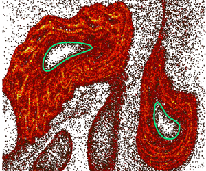
Figures 2(a) and 2(b) show the LVBs (green contours) and elliptic fixed point (red dots) identified from the TRA field, superimposed on dye-mixing patterns in the buffer and the active suspension, respectively. Although LVBs in chaotic flows are known to be transport barriers for convection (Haller et al. Reference Haller, Katsanoulis, Holzner, Frohnapfel and Gatti2020; Katsanoulis et al. Reference Katsanoulis, Farazmand, Serra and Haller2020; Aksamit & Haller Reference Aksamit and Haller2022), the LVBs in the buffer case (figure 2a) contain dye inside due to diffusion. On the other hand, the LVBs in the active case (figure 2b) enclose regions devoid of dye near the elliptic fixed points. This suggests that bacterial activity enhances the strength of LVBs as transport barriers in chaotic flows. We also notice some differences in the size and shape of the LVBs for the buffer and active cases. Since the LVBs are calculated from experimentally measured velocity fields, this indicates that microbial activity also modifies the underlying velocity field.

Figure 2. Enlarged photographs of the dye concentration field for (a) buffer and (b) active suspension, in the dashed square regions shown in figure 1. Green contours are LVBs identified from the TRA field and red dots are elliptic fixed points. (c) Dye flow rate, $\boldsymbol {J}$, as a function of time $N$, for the vortex with the label ‘4’. Inset: time-averaged dye flow rate, $\bar {\boldsymbol {J}}$, as a function of the vortex Reynolds number $Re_\varGamma$, for the buffer (blue) and the active suspension (red). Different markers represent different vortices in the flow field. Error bars are standard deviations.

To quantify the strength of the transport barriers, or the reduction in dye transport, we calculate the dye flow rate into the Lagrangian vortices using the following mass balance equation:

(3.2)\begin{equation} \frac{\mathrm{d}}{\mathrm{d}t}\int_{S(t)}C\,\mathrm{d}A = \oint_{B(t)}D(\boldsymbol{\nabla} C\boldsymbol{\cdot}\boldsymbol{n})\,\mathrm{d}l-\oint_{B(t)} C(\boldsymbol{v}-\boldsymbol{v}_{B})\boldsymbol{\cdot}\boldsymbol{n}\,\mathrm{d}l. \end{equation}

Here, $S(t)$ and $B(t)$ denote the enclosed area and the contour of the LVBs, $C$ is the dimensionless dye concentration field (normalized by the maximum fluorescence intensity), $D$ is the dye diffusivity, $\boldsymbol {n}$ is the normal vector of LVBs, $\boldsymbol {v}$ is fluid velocity and $\boldsymbol {v}_{B}$ is the velocity induced by the motion and deformation of LVBs. The first and second terms on the right-hand side of (3.2) are the surface integrals of the dye fluxes through the LVBs due to diffusion and convection, respectively. The left-hand side of (3.2) gives a simple way to calculate dye flow rate as the rate of change of the total dye enclosed by the LVBs. Figure 2(c) shows the dye flow rate, $\boldsymbol {J}$, as a function of time, for vortex with label ‘4’ in the buffer and the active suspension. We find a significant reduction of dye flow rate into the LVBs with bacterial activity, especially at earlier times ($N<150$). At later times ($N>200$), the dye flow rate in the active case is larger than that in the buffer, as a result of a larger diffusive flux due to large dye concentration gradients.

We now explore the generality of the reduction of dye flow rate in active suspensions. We start by calculating the circulation of a Lagrangian vortex, defined as

(3.3)\begin{equation} \varGamma(t) = \oint_{B(t)}\boldsymbol{v}\boldsymbol{\cdot} \mathrm{d}\boldsymbol{l}=\int_{S(t)}\omega_z\,\mathrm{d}A, \end{equation}

where $\omega _z$ denotes the vorticity component in the out-of-plane direction. We then define the the vortex Reynolds number as $Re_\varGamma = \vert \bar {\varGamma }\vert /\nu$, where $\bar {\varGamma }$ denotes the time-averaged circulation over a period, and the absolute value is included since $\bar {\varGamma }$ can be positive or negative depending on the sign of the vorticity. We calculate $Re_\varGamma$ for each Lagrangian vortex in figure 2(a,b); the labels correspond to the magnitude of their $Re_\varGamma$. The inset of figure 2(c) shows the time-averaged dye flow rate, $\bar {\boldsymbol {J}}$, as a function of the vortex Reynolds number $Re_\varGamma$, for the buffer and active cases. We find that in both cases the average dye flow rates scale linearly with $Re_\varGamma$. This is because both $\bar {\boldsymbol {J}}$ and $Re_\varGamma$ are linearly proportional to the area of the Lagrangian vortex. More importantly, however, we find that the slope of the scaling is larger in the buffer case compared with the active case. This result shows that the presence of bacteria enhances the barriers for scalar transport into the flow Lagrangian vortices.

3.2. Numerical simulations

To understand how swimming micro-organisms interact with an imposed time-periodic flow, we perform numerical simulations of swimming particles using the experimentally measured velocity field. Micro-organisms are modelled as axisymmetric ellipsoids with a constant swimming speed $v_s$, in the direction $\boldsymbol {q}$ along their symmetry axis. The swimmer's position $\boldsymbol {x}$ is modelled as

(3.4)\begin{equation} \dot{\boldsymbol{x}} = \boldsymbol{v}_f(\boldsymbol{x},t) + v_s \boldsymbol{q}, \end{equation}

where $\boldsymbol {v}_f$ is experimentally measured fluid velocity in the active suspension, and $v_s=20\ \mathrm {\mu }$m s$^{-1}$ is the swimming speed of E. coli. As a control, simulations of elongated passive particles are also performed with $v_s=0$ in the velocity field measured in the buffer. The swimmer's orientation is described by Jeffery's equation (Jeffery & Filon Reference Jeffery and Filon1922)

(3.5)\begin{equation} \dot{\boldsymbol{q}}=[\boldsymbol{W}(\boldsymbol{x}, t)+\varLambda \boldsymbol{D}(\boldsymbol{x}, t)] \boldsymbol{q}-\varLambda[\boldsymbol{q} \boldsymbol{\cdot} \boldsymbol{D}(\boldsymbol{x}, t) \boldsymbol{q}] \boldsymbol{q}, \end{equation}

where $\boldsymbol {D}$ and $\boldsymbol {W}$ are the symmetric and skew-symmetric parts of the velocity gradient tensor, $\boldsymbol {\nabla }\boldsymbol {v}_f$. Here, $\varLambda = (1-\alpha ^2)/(1+\alpha ^2)$ is a shape factor, with $\alpha$ being the swimmer's aspect ratio. We assume $\alpha =0.25$ for rod-shaped E. coli, which leads to $\varLambda \approx 0.88$.

Initially, both passive and active particles are uniformly distributed in the flow field with random orientations. As simulations begin, passive and active particles begin to develop complex patterns following the morphology of Lagrangian vortices (supplementary movie 3). Figures 3(a) and 3(b) show the spatial distribution of passive and active particles at $N=150$, respectively. The colour code in the plots represents the local particle number density, $\rho _N$, normalized by the initial number density, $\rho _0$. We find that active particles deplete within and aggregate outside the LVBs. This suggests that Lagrangian vortices repel elongated swimmers. By contrast, no depletion is observed for passive particles. Accumulation is not expected for passive particles in a two-dimensional incompressible flow, and aggregation of non-motile bacteria has not been observed in previous experiments (Ran et al. Reference Ran, Brosseau, Blackwell, Qin, Winter and Arratia2021). The accumulation of passive particles seen here is likely due to a small departure from an (ideal) divergence-free experimental velocity field (see supplementary materials). The passive particle simulation serves as a control to show that the repulsion of active particles by the Lagrangian vortices is not an intrinsic feature of the experimental velocity field itself. Rather, it is the result of the interaction between Lagrangian vortices and elongated swimmers.

Figure 3. Spatial distributions of (a) passive particles, and (b) active particles, at time $N=150$. Particles are coloured by their normalized local number density, $\rho _N/\rho _0$. Active particles are depleted from the vortex and accumulate outside the LVBs (green contours), while this depletion is not present for passive particles. (c) Radial distribution function $g(r)$ calculated from the elliptic fixed points of the Lagrangian vortex with the label ‘4’; the dashed line is the nominal radius of the vortex. (d) Spatially averaged normalized number density within the LVBs, $\langle \rho _N\rangle _S/\rho _0$, as a function of time $N$ for the same vortex as in (c).

The repulsion of rod-shaped swimmers by the LVBs is quantified by the radial distribution function: $g(r)=\langle \rho _N (r)\rangle /\rho _0$, where the angle bracket denotes a radial average in all directions calculated from the elliptic fixed points. The function $g(r)$ represents the probability of finding a particle at a radial distance $r$ from the elliptic fixed point of a Lagrangian vortex. Figure 3(c) shows $g(r)$ for both passive and active particles in the Lagrangian vortex with the label ‘4’ in figure 2. The dashed line in figure 3(c) is a nominal radius of Lagrangian vortex, defined as $r_n=\sqrt {A_S/{\rm \pi} }$, where $A_S$ is the area enclosed by the LVBs. We find that the likelihood of finding an active particle within the nominal radius of a Lagrangian vortex is smaller than that of a passive particle and vice versa for outside the nominal radius. This result further corroborates the repulsion of elongated active particles by Lagrangian vortices.

To quantify the time evolution of the repulsion of elongated swimmers, we calculate the average number density within the LVBs, $\langle \rho _N\rangle _S$, normalized by the initial number density $\rho _0$. Figure 3(d) shows $\langle \rho _N\rangle _S/\rho _0$ as a function of time $N$. Results show that $\langle \rho _N\rangle _S$ decreases non-monotonically with time for active particles, and drops to only 20 % of the initial number density $\rho _0$ at $N=200$. This suggests that most active particles escape and accumulate outside the Lagrangian vortex as mixing progresses. In the control case, $\langle \rho _N\rangle _S$ for passive particles increases with time, which again suggests the repulsion of elongated particles by LVBs is not an intrinsic feature of the velocity field itself. Although symmetric and circular Eulerian vortices have been observed to repel elongated swimmers (Torney & Neufeld Reference Torney and Neufeld2007; Ran et al. Reference Ran, Brosseau, Blackwell, Qin, Winter and Arratia2021; Qin & Arratia Reference Qin and Arratia2022), here we extend these results to a more general case of asymmetric and non-circular vortices from Lagrangian criteria.

To gain further insights into how swimming particles are repelled by Lagrangian vortices, we plot the stroboscopic trajectories and orientations of passive and active particles as a function of time, as shown in figure 4(a). The Lagrangian vortices are illustrated by the TRA field (colour map); passive and active particles are shown as blue and red bars, respectively. The trajectories of the passive particles are blue, while the trajectories of the active particles are coloured by their normalized time or number of periods, $N/N_{tot}$, where $N_{tot}$ is the total time duration of the trajectories. Despite sharing the same initial conditions for position and orientation, passive particles remain trapped in the Lagrangian vortices while active particles spiral outward with time and escape the vortices. We note that the swimming number of the active particles, $\varPhi =v_s/U$, is of the order of $10^{-2}$ in the simulations, suggesting that the swimming speed is fairly negligible compared with the flow speed. However, even such a (relatively) low swimming speed can drive active particles out of equilibrium and escape the Lagrangian vortices. That is, even small levels of swimming activity is enough to initiate the expulsion process. In addition, we find that the orientations of both passive and active particles tend to align with the level curves of the TRA field. Because the convex TRA contours locate the nested families of elliptic LCSs, this result indicates elongated particles – whether self-propelled or not – preferentially align with the members of elliptic LCSs. The difference is that the self-propulsion of active particles causes them to move outward and leave the vortices in a spiral manner.

Figure 4. (a) Stroboscopic trajectories of passive (blue) and active (red) particles that are initially inside the Lagrangian vortices illustrated by the TRA field. While sharing the same initial condition, passive particles remain trapped in the vortices and active particles spiral outward and escape. The trajectories of active particles are coloured by their normalized time (or numbers of periods), $N/N_{{tot}}$, where $N_{{tot}}$ is the total time duration of the trajectories. (b) The probability density functions (p.d.f.s) of the inner product of the particle orientation vector, $\boldsymbol {q}$, and the tangent vector of the elliptic LCSs in the direction of the vortex circulation, $\boldsymbol {t}$, as defined in the inset. The initial condition ($N=0$) is approximately a uniform distribution for particles with random initial orientations. The p.d.f.s at a later time ($N=50$) show that both passive and active particles preferentially align with members of elliptic LCSs at $\boldsymbol {q}\boldsymbol {\cdot }\boldsymbol {t}=\pm 1$. The p.d.f. of active particles is slightly biased towards the positive peak of $\boldsymbol {q}\boldsymbol {\cdot }\boldsymbol {t}=+1$. (c) Schematic of a ‘bacterial porous medium’ formed by cells aligning and accumulating outside a LVB. Dye transport is hindered as it diffuses through the porous media.

Next, we test the alignment of the elongated particles by calculating the inner product of the particle orientation vector, $\boldsymbol {q}$, and the tangent vector of the elliptic LCSs in the direction of vortex circulation, $\boldsymbol {t}$. The inset of figure 4(b) shows a schematic of the two vectors. Since elliptic LCSs are nested families, we partition the elliptic LCSs into 10 members using the convex TRA contours. The inner product is calculated between the orientation vector of an elongated particle and the tangent of the nearest member of elliptic LCSs. Figure 4(b) shows p.d.f.s of $\boldsymbol {q}\boldsymbol {\cdot }\boldsymbol {t}$ for both passive and active particles at two different times. At $N=0$, the initial condition of the p.d.f.s shared by both passive and active particles is approximately a uniform distribution due to the random initial orientations. At a later time of $N=50$, the p.d.f.s of both passive and active particles become bimodal at $\boldsymbol {q}\boldsymbol {\cdot }\boldsymbol {t}=\pm 1$, suggesting a parallel or antiparallel alignment between $\boldsymbol {q}$ and $\boldsymbol {t}$. We find that the p.d.f. of active particles shows a slight bias towards the positive peak at $\boldsymbol {q}\boldsymbol {\cdot }\boldsymbol {t}=+1$, while the bias is not present for the p.d.f. of passive particles. This suggests that active particles prefer to swim parallel to the elliptic LCSs in the direction of vortex circulation rather than swimming against the circulation. The bias in parallel and antiparallel alignments is also found for active particles of different swimming speeds (see supplementary materials). The self-propulsion of active particles can cause them to travel towards the outer members of the elliptic LCSs in both parallel and antiparallel alignment configurations (see supplementary movie 4), resulting in the spiral escaping trajectories of the active particles shown in figure 4(a). Consequently, the interplay between self-propulsion and the alignment of elongated particles with elliptic LCSs leads to the depletion of active particles inside the elliptic LCSs, that is, the accumulation of active particles outside the LVBs. This accumulation of microswimmers outside the LVBs can further obstruct dye transport into the Lagrangian vortices, which is responsible for the observed transport barriers.

3.3. Physical mechanism

We now propose a potential mechanism to explain the observed reduction in dye transport into Lagrangian vortices. We posit that the alignment and accumulation of bacteria outside the LVBs form an effective ‘bacterial porous medium’ that can impede the diffusion of dye molecules, as schematically shown in figure 4(c). In the absence of bacteria, dye should enter LVBs primarily by diffusion and marginally by inertial effect due to (low but) non-zero Reynolds number ($Re\sim 10^1$). Here, we will focus on diffusive transport around the outside boundary of the LVBs where bacteria accumulate (figure 4c). The effective diffusivity of a molecular dye through a porous medium, $D_{{eff}}$, can be estimated as follows (Grathwohl Reference Grathwohl1998)

(3.6)\begin{equation} D_{{eff}} = \frac{D_0\epsilon\delta}{\tau}, \end{equation}

where $D_0$ is the intrinsic diffusivity of the dye molecules, $\epsilon$, $\delta$ and $\tau$ are the porosity, constrictivity and tortuosity of the porous media, respectively. The porosity, $\epsilon$, is the volume fraction of the void spaces (that is, pores) in the medium relative to its total volume; $\epsilon$ ranges from 0 to 1. For our bacterial medium, the quantity $\epsilon$ sums up to unity with the bacterial volume fraction $\phi _b$ such that $\epsilon =1-\phi _b$. Bacterial accumulation around LVB leads to a local increase in $\phi _b$ of approximately tenfold (as shown by our simulations) such that $\phi _{{LVB}}\approx 10\phi _b=0.05$. Thus, the porosity of the bacterial medium is $\epsilon = 1-\phi _{{LVB}}\approx 0.95$. This leads to only a 5 % decrease in $D_{{eff}}$, which cannot account for the observed reduction in dye transport. Similarly, the constrictivity $\delta$ is a dimensionless parameter ranging from 0 to 1, which captures the hindrance to which a diffusing substance is subjected to when travelling through narrow pores. It becomes important only if the size of the diffusing molecules is comparable to that of the pores (Stenzel et al. Reference Stenzel, Pecho, Holzer, Neumann and Schmidt2016; Bini et al. Reference Bini, Pica, Marinozzi and Marinozzi2019). Here, the pore size, $O(1\ \mathrm {\mu }$m), is much greater than the molecular size, $O$(1 nm), and therefore $\delta \approx 1$. Since the values of $\delta$ and $\epsilon$ are close to unity, we do not expect them to play a significant role in the reduction of dye transport.

Next, we examine the role of tortuosity ($\tau$), which compares the (tortuous) pathway of molecular diffusion in a porous medium with its pathway in an unrestricted medium (Bini et al. Reference Bini, Pica, Marinozzi and Marinozzi2019; da Silva et al. Reference da Silva, do Rocio Cardoso, Pabst Veronese and Mazer2022). The quantity $\tau$ can be defined as (Grathwohl Reference Grathwohl1998; Holzer et al. Reference Holzer, Wiedenmann, Münch, Keller, Prestat, Gasser, Robertson and Grobéty2013; da Silva et al. Reference da Silva, do Rocio Cardoso, Pabst Veronese and Mazer2022)

(3.7)\begin{equation} \tau = \frac{\langle L_s\rangle}{L_0}, \end{equation}

where $L_0$ is the length of the straightest path and $\langle L_s\rangle$ is the ensemble average of all possible tortuous path of diffusion. Note that $\tau \ge 1$ since $\langle L_s\rangle \ge L_0$. We consider the transverse diffusion of dye molecules across a bacterial porous medium, as sketched in figure 4(c), where $x_1$ denotes the direction of the transverse diffusion and $x_2$ denotes the direction of cell body alignment with the tangent of the elliptic LCSs. During the diffusion process, each time the (dye) molecule encounters an obstacle (i.e. a bacterium), its path will be deflected by on average half the body length of a bacterium, $l_E/2$. Also, dye diffusing a distance $L_0$ (in the bacterial porous medium) will encounter bacterial cells on average $L_0\sigma _N$ times, where $\sigma _N$ is the cell number density. We can then estimate the average transverse and longitudinal path lengths, $\langle L_s\rangle _{11}$ and $\langle L_s\rangle _{22}$, for the dye to diffuse across a distance $L_0$ in the $x_1$ and $x_2$ directions as

(3.8a,b)\begin{equation} \langle L_s\rangle_{11} = L_0+L_0\sigma_Nl_E/2,\quad \langle L_s\rangle_{22} = L_0+L_0\sigma_N \alpha l_E/2, \end{equation}

where $\alpha = d_E/l_E$ is the aspect ratio between the average cell diameter $d_E$ and cell length $l_E$. For rod-shaped bacteria such as E. coli, we notice that $\alpha <1$ and thus $\langle L_s\rangle _{22}<\langle L_s\rangle _{11}$. This suggests that diffusion is anisotropic in the bacterial porous medium. We can now express the tortuosity for the transverse and longitudinal diffusion as

(3.9a,b)\begin{equation} \tau_{11} = \frac{\langle L_s\rangle_{11}}{L_0}= 1+\sigma_N l_E/2,\quad \tau_{22} = \frac{\langle L_s\rangle_{22}}{L_0}= 1+\alpha\sigma_N l_E/2. \end{equation}

In our experiments, the local bacterial volume fraction (around LVBs) is $\phi _{{LVB}}\approx 0.05$, which corresponds to a local cell number density of $\rho _N \approx 1.25\times 10^{11}$ cells ml$^{-1}$, and a local cell number density of $\sigma _N \approx 5000$ cells cm$^{-1}$. If we consider $l_E$ to be the bacterium body length (${\approx }2\ \mathrm {\mu }$m), then $\tau _{11} = 1+\sigma _N l_E/2=1.5$. If instead we consider the ‘total’ bacterium length (cell body plus flagella), $L_{{total}}\approx 7\ \mathrm {\mu }$m (Patteson et al. Reference Patteson, Gopinath, Goulian and Arratia2015), then $\tau _{11} = 1+\sigma _N L_{{total}}/2=2.75$. Using the above estimates, we expect $1.5\le \tau _{11}\le 2.75$. The transverse effective diffusivity can be estimated using (3.6), and this yields $0.346\le D_{11}/D_0\le 0.633$. Therefore, a dye diffusing through this bacterial porous media would experience a 33 %–66 % decrease in the transverse effective diffusivity, which qualitatively corresponds to the decrease in dye transport into the LVBs. Note that (3.9a,b) estimates an anisotropic diffusivity, $D_{11}< D_{22}$, for rod-shaped bacteria ($\alpha <1$). Bacterial flagellar motion, in addition, can displace dye molecules farther in the $x_2$ direction, which would lead to an increase in $D_{22}$. This would lead to a more complex behaviour than the one described here. Nevertheless, the concept of anisotropic diffusion in a bacterial porous media seems to capture, at least qualitatively, the observed decrease in scalar transport into the Lagrangian vortices.