


Introduction
The main objective of the present paper is to investigate the existence and the sources of economies of diversification in French mixed sheep farms and to identify mixtures of sheep farming activities that provide greater risk-adjusted returns to farmers. Such an analysis may be useful for producers who think about changing their production mix. In fact, we are interested in two standard economic rationales for diversification strategies. Indeed, in economics it is usually argued that production diversification can have (or can be driven by) two effects: a risk-reducing effect and a scope economies effect (Chavas and Di Falco Reference Chavas and Di Falco2012). Under uncertainty, risk-averse producers have incentives to diversify their production activities (Heady Reference Heady1952). This could be explained by the fact that production diversification can be seen as a strategy used by farmers to protect themselves against production and market risks. Since farmers are typically risk-averse (they are aware of the variability in their productions and their related prices), they may respond to risk by diversifying their production activities. This could be illustrated by the rule of thumb: “Don’t put all your eggs in one basket” (Chavas and Di Falco Reference Chavas and Di Falco2012, p. 26). Diversification can thus help farms to be more resilient (i.e., to withstand external shocks without catastrophic consequences or to absorb downside shocks) in case of a crisis in at least one of their production activities.
Besides risk management, another possible motivation for diversification is the presence of economies of scope (Chavas and Di Falco Reference Chavas and Di Falco2012). Scope economies exist if the cost of joint production of a set of outputs in a diversified firm is lower than the cost of their disjoint production in several specialized firms. The concept of economies of scope focuses on measuring economic gains (in terms of cost reductions) associated with diversified firms in comparison with specialized firms. Analysis of scope economies requires either data on completely specialized firms (or stand-alone production) or partitions of the outputs of the firms in mutually exclusive categories (see, Panzar and Willig Reference Panzar and Willig1981; Grosskopf, Hayes, and Yaisawarng Reference Grosskopf, Hayes and Yaisawarng1992; Ferrier et al. Reference Ferrier, Grosskopf, Hayes and Yaisawarng1993). Since such data are not always available, the classic definition of economies of scope has been generalized to economies of diversification (Grosskopf, Hayes, and Yaisawarng Reference Grosskopf, Hayes and Yaisawarng1992; Ferrier et al. Reference Ferrier, Grosskopf, Hayes and Yaisawarng1993; Chavas and Kim Reference Chavas and Kim2010; Chavas and Di Falco Reference Chavas and Di Falco2012; Malikov, Zhao, and Kumbhakar Reference Malikov, Zhao and Kumbhakar2017). Economies of diversification measure economic gains (in terms of cost reductions or certainty equivalents) associated with fully diversified firms in comparison with partially diversified firms. Thus, economies of scope are a special case of the more general measure of economies of diversification (Eder Reference Eder2018).
Empirically, these two effects are usually investigated separately (e.g., Smale et al. Reference Smale, Hartell, Heisey and Senauer1998; Di Falco and Chavas Reference Di Falco and Chavas2009). Recently, Chavas and Di Falco (Reference Chavas and Di Falco2012) introduced a unified framework where both rationales for production diversification are integrated into an applied microeconomics setting using the concept of certainty equivalent (CE). Our paper uses their approach but it departs from Chavas and Di Falco (Reference Chavas and Di Falco2012) in three ways. First, in contrast to Chavas and Di Falco (Reference Chavas and Di Falco2012), our analysis is based on observed partially diversified farms (see also, Malikov, Zhao, and Kumbhakar Reference Malikov, Zhao and Kumbhakar2017). Second, while Chavas and Di Falco (Reference Chavas and Di Falco2012) consider only production risk, we consider both yield and price risks. Third, we apply the Stochastic Efficiency with respect to a Function (SERF) method (Hardaker et al. Reference Hardaker, Richardson, Lien and Schumann2004), which is widely used to estimate CE values and to compare risky alternatives. As such, our framework has two important features. First, it makes it possible to investigate the existence and the sources of economies of diversification. Second, it allows a ranking of farming activities in terms of stochastic dominance. The SERF method has been used previously to rank crop production systems (e.g., Pendell et al. Reference Pendell, Williams, Boyles, Rice and Nelson2007; Watkins, Hill, and Anders Reference Watkins, Hill and Anders2008; Bryant et al. Reference Bryant, Reeves, Nichols, Greene, Tingle, Studebaker, Bourland, Capps and Groves2008; Archer and Reicosky Reference Archer and Reicosky2009; Williams et al. Reference Williams, Gollany, Siemens, Wuest and Long2009; Hignight, Watkins, and Anders Reference Hignight, Watkins and Anders2010; Barham et al. Reference Barham, Robinson, Richardson and Rister2011; Williams et al. Reference Williams, Pachta, Roozeboom, Llewelyn, Claassen and Bergtold2012; Boyer et al. Reference Boyer, Lambert, Larson and Tyler2018; Adusumilli et al. Reference Adusumillia, Wanga, Dodlab and Deliberto2020). However, to our best knowledge, our paper provides the first application of the SERF method in economics of diversification.
Our framework is applied to a sample of sheep farms in an area in the Center of France, namely the “Massif Central.” Besides their main activity (sheep), some farms in the Massif Central have complementary activities (e.g., crop, landless activities). These activities have been developed given, inter alia, market opportunity, difficulties in the sheep sector, and available labor force. Under the European terminology, the Massif Central is classified as a Less Favored Agricultural Area. In these areas, farmers operate under more difficult production conditions, such as steep lands, high altitudes, unfavorable climates (e.g., short growing season and long wintering period), and isolated locations. The Massif Central includes mountain areas (60% of the territory); but also areas immediately adjacent to them, which are known as simple less-favored areas (foothills, plains) (SIDAM 2020)Footnote 1 . Eighty-five percent of the territory of the Massif Central is devoted to grazing livestock, including 60% of permanent grassland (SIDAM 2020). In the Massif Central, sheep farming represents the third agricultural production activity in terms of farm numbers (15% of farms), after beef cattle farming (38% of farms) and dairy cattle farming (20% of farms) (SIDAM 2020) (see also appendix A). An advantage of sheep farming is that sheep are well suited to valorize Less Favored Agricultural Areas, such as the Massif Central (Benoit and Laignel Reference Benoit and Laignel2009). However, the sheep farms in the Massif Central are exposed to hazards (climate, health, etc.), but also to seasonal and annual price volatility (see appendix B). In this context, our analysis may provide relevant information for designing/selecting mixtures of farming activities that allow farmers to have greater risk-adjusted returns, to reduce their economic risk (including downside risk exposure), or to valorize territorial potentialities (including touristic activities) of the Massif Central.
The remainder of the paper is organized as follows. The second section describes our analytical approach. The third section presents the data used. Results are presented and discussed in the fourth section, and the fifth section provides concluding remarks.
Theoretical, conceptual, and empirical considerations
The Expected Utility Theory and the concept of Certainty Equivalent
Our analysis is based on the concept of Certainty Equivalent (CE), which is derived from the Expected Utility Theory (EUT). The EUT postulates that when faced with risky prospects, an individual chooses the alternative that offers the maximum expected utility. Under this theory, the preferences of economic agents are represented by a utility function U(.), and the consequences of their decisions by random variables $\pi $
associated with probabilities p. The EUT assumes that agents make their decisions as if they were maximizing the expected utility of their random earnings. Thus, they prefer a random gain
$\pi $
associated with probabilities p. The EUT assumes that agents make their decisions as if they were maximizing the expected utility of their random earnings. Thus, they prefer a random gain ${\pi _1}$
to a random gain
${\pi _1}$
to a random gain ${\pi _2}$
,
${\pi _2}$
, ${\pi _1}$ $\geq$ ${\pi _2}$
, if and only if
${\pi _2}$
, if and only if $EU\left( {{\pi _1}} \right) \ge EU\left( {{\pi _2}} \right)$
.
$EU\left( {{\pi _1}} \right) \ge EU\left( {{\pi _2}} \right)$
.
More formally, denote by $U\left( \pi \right)$
the utility function of a producer with respect to stochastic outcomes (
$U\left( \pi \right)$
the utility function of a producer with respect to stochastic outcomes ( $\pi $
) (e.g., random net returns). The probability density functions (PDF) that represent the outcomes for n risky alternatives are noted by
$\pi $
) (e.g., random net returns). The probability density functions (PDF) that represent the outcomes for n risky alternatives are noted by ${f_1}\left( \pi \right),{f_2}\left( \pi \right), \ldots ,\;{f_n}\left( \pi \right)$
, and their corresponding cumulative distribution functions (CDF) are
${f_1}\left( \pi \right),{f_2}\left( \pi \right), \ldots ,\;{f_n}\left( \pi \right)$
, and their corresponding cumulative distribution functions (CDF) are ${F_1}\left( \pi \right),{F_2}\left( \pi \right), \ldots ,\;{F_n}\left( \pi \right)$
. The utility of these alternatives can be expressed as follows:
${F_1}\left( \pi \right),{F_2}\left( \pi \right), \ldots ,\;{F_n}\left( \pi \right)$
. The utility of these alternatives can be expressed as follows:
 $$U\left( \pi \right) = EU\left( \pi \right) = \int U\left( \pi \right)f\left( \pi \right)d\pi = \int U\left( \pi \right)dF\left( \pi \right)$$
From the CDF, it is possible to determine which alternative is stochastically dominant. For instance, given two alternatives A and B, with CDFs over outcomes $\pi $
defined by
$\pi $
defined by ${F_a}\left( \pi \right)$
and
${F_a}\left( \pi \right)$
and ${F_b}\left( \pi \right)$
, alternative A will dominate alternative B if
${F_b}\left( \pi \right)$
, alternative A will dominate alternative B if ${F_a}\left( \pi \right) \le {F_b}\left( \pi \right)$
. Graphically, this means that
${F_a}\left( \pi \right) \le {F_b}\left( \pi \right)$
. Graphically, this means that ${F_b}\left( \pi \right)$
is closest to the origin of the axes. In other words, the CDF of A must be to the right of the CDF of B. However, for more discriminating power, we will rank our mixed sheep farms by converting their utility into certainty equivalents (CE) as follows (Hardaker et al. Reference Hardaker, Richardson, Lien and Schumann2004; Hardaker et al. Reference Hardaker, Lien, Anderson and Huirne2015):
${F_b}\left( \pi \right)$
is closest to the origin of the axes. In other words, the CDF of A must be to the right of the CDF of B. However, for more discriminating power, we will rank our mixed sheep farms by converting their utility into certainty equivalents (CE) as follows (Hardaker et al. Reference Hardaker, Richardson, Lien and Schumann2004; Hardaker et al. Reference Hardaker, Lien, Anderson and Huirne2015):
 $$CE\left( \pi \right) = {U^{ - 1}}\left[ {EU\left( \pi \right)} \right]$$
where ${U^{ - 1}}$
is the reciprocal of the utility function
${U^{ - 1}}$
is the reciprocal of the utility function $U$
.
$U$
.
Existence of diversification economies
Following Chavas and Di Falco (Reference Chavas and Di Falco2012), economies of diversification (diseconomies of diversification) (ED) exist if:
 $$ED = \;CE\left( \pi \right) - \mathop \sum \nolimits_{k = 1}^K CE\left( {{\pi _k}} \right)\; \gt 0\left( { \lt 0} \right)\;$$
where $CE\left( \pi \right)$
is the certainty equivalent value of the net return of the fully diversified farms and
$CE\left( \pi \right)$
is the certainty equivalent value of the net return of the fully diversified farms and $CE\left( {{\pi _k}} \right)$
is the certainty equivalent value of the net return of the k-th type of partially diversified farms. As aforementioned, in contrast to Chavas and Di Falco (Reference Chavas and Di Falco2012), our counterfactual
$CE\left( {{\pi _k}} \right)$
is the certainty equivalent value of the net return of the k-th type of partially diversified farms. As aforementioned, in contrast to Chavas and Di Falco (Reference Chavas and Di Falco2012), our counterfactual $CE\left( {{\pi _k}} \right)$
is defined on observed partially diversified farms (see also, Malikov, Zhao, and Kumbhakar Reference Malikov, Zhao and Kumbhakar2017). The variable
$CE\left( {{\pi _k}} \right)$
is defined on observed partially diversified farms (see also, Malikov, Zhao, and Kumbhakar Reference Malikov, Zhao and Kumbhakar2017). The variable ${\pi _k}$
is the net income of the k-th type of partially diversified farms, that is, it is measured as the profit generated by all the activities of this kind of farm. For instance, for the Sheep-Crop system, it is measured as the sum of the profit generated by the sheep and the crop production.
${\pi _k}$
is the net income of the k-th type of partially diversified farms, that is, it is measured as the profit generated by all the activities of this kind of farm. For instance, for the Sheep-Crop system, it is measured as the sum of the profit generated by the sheep and the crop production.
Equation (3) indicates that economies of diversification exist (ED > 0) when the certainty equivalent of the fully diversified farms is higher than the one of K partially diversified farms. This may allow us to identify the presence of positive externalities across production activities. Alternatively, diseconomies of diversification exist if ED < 0.
Equation (3) provides a monetary measure of diversification benefits. Assuming that $CE\left( \pi \right) \gt 0$
, a relative measure that provides the degree of diversification economies can be defined using the following expression:
$CE\left( \pi \right) \gt 0$
, a relative measure that provides the degree of diversification economies can be defined using the following expression:
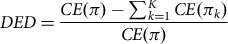 $$DED = \displaystyle{{CE\left( \pi \right) - \sum\nolimits_{k = 1}^K C E\left( {{\pi _k}} \right)} \over {CE\left( \pi \right)}}$$
The components of diversification economies
For a stochastic outcome, $\pi $
, Pratt (Reference Pratt1964) has shown that the CE can be approximated by:
$\pi $
, Pratt (Reference Pratt1964) has shown that the CE can be approximated by:
 $$CE\left[ \pi \right]\;\; = \;E\left[ \pi \right]-R\left( \pi \right)$$
where $E\left[ \pi \right]$
denotes the expected value of
$E\left[ \pi \right]$
denotes the expected value of $\pi $
and
$\pi $
and $R\left( \pi \right)$
is a risk premium. Thus, the certainty equivalent of a random outcome
$R\left( \pi \right)$
is a risk premium. Thus, the certainty equivalent of a random outcome $\pi $
,
$\pi $
, $CE\left[ \pi \right]$
, is the difference between its expected value (
$CE\left[ \pi \right]$
, is the difference between its expected value ( $E\left[ \pi \right]$
) and a risk premium
$E\left[ \pi \right]$
) and a risk premium $\;R\left( \pi \right)$
. The risk premium (R) is the maximum amount of money that a risk-averse individual is willing to pay to avoid facing a risk. In other words, it is the amount of money that a risk-averse farmer is willing to give up to eliminate risk exposure. That is, the risk premium is the implicit cost of risk bearing. From equation (5), the CE can be seen as the risk-adjusted value of the expected net return. Equation (5) has been used by Chavas and Di Falco (Reference Chavas and Di Falco2012) to derive the components of diversification economies. In this respect, economies of diversification (diseconomies of diversification) (ED) exist if:
$\;R\left( \pi \right)$
. The risk premium (R) is the maximum amount of money that a risk-averse individual is willing to pay to avoid facing a risk. In other words, it is the amount of money that a risk-averse farmer is willing to give up to eliminate risk exposure. That is, the risk premium is the implicit cost of risk bearing. From equation (5), the CE can be seen as the risk-adjusted value of the expected net return. Equation (5) has been used by Chavas and Di Falco (Reference Chavas and Di Falco2012) to derive the components of diversification economies. In this respect, economies of diversification (diseconomies of diversification) (ED) exist if:
 $$ED = \;E{D_\pi } + E{D_R}\; > 0{\mkern 1mu} ( < 0)$$
Where
 $$E{D_\pi } = E\left[ \pi \right] - \mathop \sum \limits_{k = 1}^K E\left[ {{\pi _k}} \right]$$
 $$E{D_R} = - \left[ {R\left( \pi \right) - \mathop \sum \limits_{k = 1}^K R\left( {{\pi _k}} \right)} \right]$$
Equation (6) identifies two additive components of the benefits of diversification: the expected income component $E{D_\pi }$
, and the risk component
$E{D_\pi }$
, and the risk component $E{D_R}$
. The risk premium estimated from the SERF method can be used in the equation of
$E{D_R}$
. The risk premium estimated from the SERF method can be used in the equation of $E{D_R}$
to examine the risk component of diversification economies. However, following Chavas and Di Falco (Reference Chavas and Di Falco2012) we use the variance component and the skewness component of the risk premium separately in order to examine the effects of diversification patterns on different aspects of risk exposure. As such, given the utility function
$E{D_R}$
to examine the risk component of diversification economies. However, following Chavas and Di Falco (Reference Chavas and Di Falco2012) we use the variance component and the skewness component of the risk premium separately in order to examine the effects of diversification patterns on different aspects of risk exposure. As such, given the utility function $U\left( \pi \right)$
, the risk premium can be expressed as follows (Chavas Reference Chavas2004; Chavas and Di Falco [Reference Chavas and Di Falco2012]):
$U\left( \pi \right)$
, the risk premium can be expressed as follows (Chavas Reference Chavas2004; Chavas and Di Falco [Reference Chavas and Di Falco2012]):
 $$R\left( \pi \right) = - {1 \over 2}{{U_\pi ^{''}} \over {U_\pi ^{'}}}{\rm{Var}}\left( \pi \right) - {1 \over 6}{{U_\pi ^{'}} \over {U_\pi ^{'}}}{\rm{Skew}}\left( \pi \right)$$
where $U_\pi ^h$
denotes the derivative of order
$U_\pi ^h$
denotes the derivative of order $h$
of the utility function with respect to
$h$
of the utility function with respect to $\pi $
.
$\pi $
. $ - U''/U'$
is known as the Arrow–Pratt risk aversion coefficient and
$ - U''/U'$
is known as the Arrow–Pratt risk aversion coefficient and $U'''/U'$
is a measure of downside risk aversion. From equation (7), the risk premium can be decomposed into two components:
$U'''/U'$
is a measure of downside risk aversion. From equation (7), the risk premium can be decomposed into two components:
 $$R\left( \pi \right) = {R_{{\rm{Var}}}} + {R_{{\rm{Skew}}}}$$
where
 $${R_{{\rm{Var}}}} = - {1 \over 2}{{U_\pi ^{''}} \over {U_\pi ^{'}}}{\rm{Var}}\left( \pi \right)$$
is the variance component and
$${R_{{\rm{Var}}}} = - {1 \over 2}{{U_\pi ^{''}} \over {U_\pi ^{'}}}{\rm{Var}}\left( \pi \right)$$
is the variance component and
 $${R_{{\rm{Skew}}}} = - {1 \over 6}{{U_\pi ^{'}} \over {U_\pi ^{'}}}{\rm{Skew}}\left( \pi \right)$$
is the skewness component of the risk premium. As previously mentioned, the variance component and the skewness component can be used separately in the
$${R_{{\rm{Skew}}}} = - {1 \over 6}{{U_\pi ^{'}} \over {U_\pi ^{'}}}{\rm{Skew}}\left( \pi \right)$$
is the skewness component of the risk premium. As previously mentioned, the variance component and the skewness component can be used separately in the $E{D_R}$
equation to examine the variance and the skewness effects of diversification economies. However, from an empirical standpoint, it is difficult to derive the variance and the skewness components from the SERF estimatesFootnote
2
. Indeed, in its current form, the SERF method provides the Arrow-Pratt risk aversion coefficients and not the downside risk aversion coefficients. Hence, in this sub-section, we focus mainly on the variance component, while special attention is devoted to the skewness component in the next sub-section. In the estimation of the variance component, the risk aversion coefficients
$E{D_R}$
equation to examine the variance and the skewness effects of diversification economies. However, from an empirical standpoint, it is difficult to derive the variance and the skewness components from the SERF estimatesFootnote
2
. Indeed, in its current form, the SERF method provides the Arrow-Pratt risk aversion coefficients and not the downside risk aversion coefficients. Hence, in this sub-section, we focus mainly on the variance component, while special attention is devoted to the skewness component in the next sub-section. In the estimation of the variance component, the risk aversion coefficients
 $$\left( {{{U_\pi ^{''}} \over {U_\pi ^{'}}}} \right)$$
are obtained from the SERF method and the variance (
$$\left( {{{U_\pi ^{''}} \over {U_\pi ^{'}}}} \right)$$
are obtained from the SERF method and the variance ( ${\rm{Var}}\left( \pi \right)$
) is estimated using econometric techniques as in Chavas and Di Falco (2012) (see the next sub-section for more details).
${\rm{Var}}\left( \pi \right)$
) is estimated using econometric techniques as in Chavas and Di Falco (2012) (see the next sub-section for more details).
Diversified production systems and downside risk exposure
In the previous sub-section, we focused mainly on the variance component of the risk component of the diversification economies. However, since the variance does not distinguish between unexpected good and bad events, that is, between upside and downside risk (Di Falco and Chavas Reference Di Falco and Chavas2009), special attention is devoted here to the skewness component. Indeed, we use the third moment (the skewness) of farmers’ income distribution ( ${\rm{Skew}}\left( \pi \right)$
) for downside risk exposureFootnote
3
analysis to provide additional information for diversification strategies (Antle Reference Antle1983; Kim and Chavas Reference Kim and Chavas2003; Donoso Reference Donoso2014; Bozzola and Finger Reference Bozzola and Finger2021). That is, we assume that higher moments than the variance play an important role in farmers’ decision process. This is in line with the fact that agricultural returns are often characterized by extreme loss events and farmers are often downside risk-averse (Menezes, Geiss, and Tressler Reference Menezes, Geiss and Tressler1980; Antle Reference Antle1983; Di Falco and Chavas Reference Di Falco and Chavas2006; Koundouri, Laukkanen, and Myyra Reference Koundouri, Laukkanen and Myyra2009). In an agricultural setting, the downside risk is particularly relevant as it identifies the probability of failure. Indeed, an increase in the skewness of the income means that downside risk exposure decreases, that is, the probability of failure decreases (Di Falco and Chavas Reference Di Falco and Chavas2009). This suggests that an increase in the downside risk involves an increase in the skewness of the risk distribution toward low outcomes (Menezes, Geiss, and Tressler Reference Menezes, Geiss and Tressler1980). By definition, a downside risk-averse decision maker is impoverished by such a change (Di Falco and Chavas Reference Di Falco and Chavas2006). In this respect, farmers exhibiting downside risk aversion have incentives to develop management strategies that affect positively the skewness of the distribution of their returns, thus reducing their exposure to downside risk (i.e., by reducing the probability of failure) (Di Falco and Chavas Reference Di Falco and Chavas2006).
${\rm{Skew}}\left( \pi \right)$
) for downside risk exposureFootnote
3
analysis to provide additional information for diversification strategies (Antle Reference Antle1983; Kim and Chavas Reference Kim and Chavas2003; Donoso Reference Donoso2014; Bozzola and Finger Reference Bozzola and Finger2021). That is, we assume that higher moments than the variance play an important role in farmers’ decision process. This is in line with the fact that agricultural returns are often characterized by extreme loss events and farmers are often downside risk-averse (Menezes, Geiss, and Tressler Reference Menezes, Geiss and Tressler1980; Antle Reference Antle1983; Di Falco and Chavas Reference Di Falco and Chavas2006; Koundouri, Laukkanen, and Myyra Reference Koundouri, Laukkanen and Myyra2009). In an agricultural setting, the downside risk is particularly relevant as it identifies the probability of failure. Indeed, an increase in the skewness of the income means that downside risk exposure decreases, that is, the probability of failure decreases (Di Falco and Chavas Reference Di Falco and Chavas2009). This suggests that an increase in the downside risk involves an increase in the skewness of the risk distribution toward low outcomes (Menezes, Geiss, and Tressler Reference Menezes, Geiss and Tressler1980). By definition, a downside risk-averse decision maker is impoverished by such a change (Di Falco and Chavas Reference Di Falco and Chavas2006). In this respect, farmers exhibiting downside risk aversion have incentives to develop management strategies that affect positively the skewness of the distribution of their returns, thus reducing their exposure to downside risk (i.e., by reducing the probability of failure) (Di Falco and Chavas Reference Di Falco and Chavas2006).
We are concerned with the question of how diversification affects the third central moment (the skewness) of the distribution of farm income or whether diversified systems could help farmers to reduce their exposure to downside risk. We use an econometric moment-based approach to this assessment (Antle, Reference Antle1983; Chavas and Di Falco Reference Chavas and Di Falco2012). This approach has been widely used in the context of risk management in agriculture (Kim and Chavas Reference Kim and Chavas2003; Koundouri, Nauges, and Tzouvelekas Reference Koundouri, Nauges and Tzouvelekas2006; Bozzola and Finger Reference Bozzola and Finger2021). In order to specify the econometric model, we rewrite the CE as follows (Di Falco and Chavas Reference Di Falco and Chavas2006):
 $$CE = E\left[ {p{\rm{g}}\left( {x,z} \right)} \right] - C\left( {x,z} \right) - R\left( {x,z} \right)$$
Where $p$
is a vector of output prices and
$p$
is a vector of output prices and ${\rm{g}}\left(. \right)$
is a production function. Equation (9) indicates that production factors (
${\rm{g}}\left(. \right)$
is a production function. Equation (9) indicates that production factors ( $x$
) and contextual drivers (or management decisions) (
$x$
) and contextual drivers (or management decisions) ( $z$
) can affect the expected revenueFootnote
4
(
$z$
) can affect the expected revenueFootnote
4
( $E\left[ {p{\rm{g}}\left( {x,z} \right)} \right]$
), the production cost (
$E\left[ {p{\rm{g}}\left( {x,z} \right)} \right]$
), the production cost ( $C\left( {x,z} \right))$
as well as the risk premium (
$C\left( {x,z} \right))$
as well as the risk premium ( $R\left( {x,\;z} \right)$
). It is worth noting that from equations (7) and (9), the risk premium is given by
$R\left( {x,\;z} \right)$
). It is worth noting that from equations (7) and (9), the risk premium is given by $R\left( {x,z} \right) = {1 \over 2}{{U_\pi ^{''}} \over {U_\pi ^{'}}}{\rm{Var}}\left( {\pi \left( {x,z} \right)} \right) - {1 \over 6}{{U_\pi ^{'''}} \over {U_\pi ^{'}}}{\rm{Skew}}\left( {\pi \left( {x,z} \right)} \right)$
, implying that
$R\left( {x,z} \right) = {1 \over 2}{{U_\pi ^{''}} \over {U_\pi ^{'}}}{\rm{Var}}\left( {\pi \left( {x,z} \right)} \right) - {1 \over 6}{{U_\pi ^{'''}} \over {U_\pi ^{'}}}{\rm{Skew}}\left( {\pi \left( {x,z} \right)} \right)$
, implying that $x$
and
$x$
and $z$
can also affect the variance and the skewness components.
$z$
can also affect the variance and the skewness components.
The econometric estimations follow a two-step procedure. In the first step, the income is regressed on production factors ( $x$
) and contextual drivers (
$x$
) and contextual drivers ( $z$
) to provide an estimate of the “mean” (i.e., the first moment) effect:
$z$
) to provide an estimate of the “mean” (i.e., the first moment) effect:
 $$\pi = {f_1}\left( {x,z} \right) + \upsilon $$
where $\pi $
is the farm income per hectare,
$\pi $
is the farm income per hectare, $x$
is a vector of production factors (labor, farm capital, intermediate inputs), and
$x$
is a vector of production factors (labor, farm capital, intermediate inputs), and $z$
is a vector of contextual drivers (Latruffe et al., Reference Latruffe, Minviel and Salanié2013) including farm-specific characteristics (e.g., diversification patterns, feed autonomy). In equation (10),
$z$
is a vector of contextual drivers (Latruffe et al., Reference Latruffe, Minviel and Salanié2013) including farm-specific characteristics (e.g., diversification patterns, feed autonomy). In equation (10), ${f_1}\left( {x,z} \right) = E\left[ \pi \right]$
is the mean of
${f_1}\left( {x,z} \right) = E\left[ \pi \right]$
is the mean of $\pi $
, and
$\pi $
, and $\upsilon = \pi - {f_1}\left( {x,z} \right)$
is the usual identically independently distributed error term. In the second step, higher-order momentsFootnote
5
of the income are given by:
$\upsilon = \pi - {f_1}\left( {x,z} \right)$
is the usual identically independently distributed error term. In the second step, higher-order momentsFootnote
5
of the income are given by:
 $$E\left[ {{{\left( {\pi - {f_1}\left( {x,z} \right)} \right)}^k}} \right] = {f_k}\left( {x,z} \right) + \tilde \upsilon ,k = 2,\!3$$
Thus, ${f_2}\left( {x,z} \right)$
represents the second central moment (the variance), and
${f_2}\left( {x,z} \right)$
represents the second central moment (the variance), and ${f_3}\left( {x,\;z} \right)$
is the third central moment (the skewness). Equations (10) and (11) can be consistently estimated using least-squares methods (Kim and Chavas Reference Kim and Chavas2003; Koundouri, Nauges, and Tzouvelekas Reference Koundouri, Nauges and Tzouvelekas2006).
${f_3}\left( {x,\;z} \right)$
is the third central moment (the skewness). Equations (10) and (11) can be consistently estimated using least-squares methods (Kim and Chavas Reference Kim and Chavas2003; Koundouri, Nauges, and Tzouvelekas Reference Koundouri, Nauges and Tzouvelekas2006).
The SERF method
The SERF method has been developed to estimate the certainty equivalent (CE) of the return of a set of risky alternatives in order to rank them over a range of risk aversion coefficients. In the present study, we also used the CE values estimated with the SERF method to investigate the existence and the components of economies of diversification for our sample of mixed sheep farms.
The SERF method estimates the CE values using equations (1) and (2). It therefore requires the specification of a utility function. Schumann et al. (Reference Schumann, Richardson, Lien and Hardaker2004) showed that the use of different types of utility functions, such as the power or negative exponential utility functions, is unlikely to affect the results of the SERF method. In this study, we use the power utility function to estimate the CE values. This utility function exhibits a decreasing absolute risk aversion, namely individuals are willing to take more risks when their wealth increases. In the implementation of the SERF method, we do not need to know the decision-maker’s risk aversion coefficient $\phi $
(Richardson and Outlaw Reference Richardson and Outlaw2008). It requires only to set a lower and an upper value for
$\phi $
(Richardson and Outlaw Reference Richardson and Outlaw2008). It requires only to set a lower and an upper value for $\phi $
(e.g.,
$\phi $
(e.g., $\phi = 0$
, for risk-neutral producers and
$\phi = 0$
, for risk-neutral producers and $\phi = 4$
, for extremely risk-averse producers) (see Anderson and Dillon Reference Anderson and Dillon1992). This enables the SERF method to rank risky alternatives upon a plausible range of risk aversion coefficients (Schumann et al. Reference Schumann, Richardson, Lien and Hardaker2004). This is an important point because producers with different degrees of risk aversion are likely to have different preferences among risky alternatives (Hardaker, Huirne, and Anderson Reference Hardaker, Huirne and Anderson1997).
$\phi = 4$
, for extremely risk-averse producers) (see Anderson and Dillon Reference Anderson and Dillon1992). This enables the SERF method to rank risky alternatives upon a plausible range of risk aversion coefficients (Schumann et al. Reference Schumann, Richardson, Lien and Hardaker2004). This is an important point because producers with different degrees of risk aversion are likely to have different preferences among risky alternatives (Hardaker, Huirne, and Anderson Reference Hardaker, Huirne and Anderson1997).
The SERF method has many advantages over other methods usually used for comparing risky alternatives. For instance, the direct implementation of the expected utility approach requires consistent specification of the utility function of the decision maker (Anderson, Dillon, and Hardaker Reference Anderson, Dillon and Hardaker1977). However, it has been shown that accurate elicitation of the utility function of the decision makers is not a clear-cut issue (King and Robison Reference King, Robison and Barry1984). First-order and second-order stochastic dominance overcome the need to define a utility function, but they often lead to meaningless results (Schumann et al. Reference Schumann, Richardson, Lien and Hardaker2004). Another approach, called stochastic dominance with respect to a function (SDRF) could be used to compare risky alternatives (Meyer Reference Meyer1977). The SDRF method does not require an explicit definition of a utility function, but only a lower and an upper absolute risk aversion coefficient. However, the SDRF method performs only pairwise comparisons (Hardaker et al. Reference Hardaker, Richardson, Lien and Schumann2004). The mean-variance (MV) method could also be used to compare risky alternatives. However, the MV approach often leads to inconclusive results (Hardaker et al. Reference Hardaker, Richardson, Lien and Schumann2004). The SERF method overcomes the limitations of the previous methods. In addition, unlike the SDRF, the SERF method compares simultaneously many risky alternatives (Hardaker et al. Reference Hardaker, Richardson, Lien and Schumann2004; Meyer, Richardson, and Schumann Reference Meyer, Richardson and Schumann2009). Another advantage of the SERF method is that it considers the entire distribution of the net return, but not only one point of measurement, as does the MV method.
In SERF analysis, the term stochastic efficiency is usually used to interpret the results. However, in the present study, to avoid any confusion with the term stochastic frontier analysis (SFA) commonly used in efficiency analysis (Minviel and Sipiläinen Reference Minviel and Sipiläinen2018; Minviel and Sipiläinen Reference Minviel and Sipiläinen2021), we use the term stochastic dominance. Indeed, we acknowledge that SERF is a variant (an improved method or a generalized form) of stochastic dominance analysis (see also, Schenk et al. Reference Schenk, Hellegers, van Asseldonk and Davidson2014). Note also that the SERF procedure is suggested to be a method of stochastic dominance analysis (Meyer, Richardson, and Schumann Reference Meyer, Richardson and Schumann2009; Hardaker and Lien Reference Hardaker and Lien2010). This is related to the fact that stochastic dominance analysis is often used to order risky prospects (Lien Reference Lien2003).
Data description
The data used in this study come from surveys carried out by the Joint Research Unit Herbivores (UMRH), of the French National Research Institute for Agriculture, Food and the Environment (INRAE). These data were collected in a network of suckler sheep farms monitored annually over the period 1987 to 2017. During these successive surveys, many variables were collected on the structure and management of the flock, as well as on the technical and economic results of the farms. More precisely, our dataset includes information on: (i) the workforce (family, salaried, temporary); (ii) the flock (lambing, animal movements, and weights of animals sold); (iii) areas (crops, grassland); (iv) equipment (exhaustive list and costs); (v) buildings and installations; (vi) intermediate consumption (quantities and prices); (vii) sales (types of animals and crops, quantities, prices); (viii) subsidies (coupled, decoupled, unit amounts); and (ix) investments, loans, social contributions, taxes, salaries paid, and insurance. The farms are mainly located in the north of the Massif Central and its periphery, and they are distributed between plain areas with grassland breeds and mountain and foothill areas with rustic breeds.
Our empirical analysis is undertaken on an unbalanced panel of 1,139 farm-year observations from 134 mixed sheep farms over the period from 1987 to 2017. Over this period, we keep farms that were surveyed for at least 3 years in order to have a certain level of variability in the data. Based on the strategies used by farmers to mitigate economic risks, the following sheep farming systems are examined in the present study:
-
Sheep-Grass: This system consists of farms that have neither annual crops nor other livestock. These are farms with 100% of their land dedicated to grass.
-
Sheep-Crop: This system concerns farms that have sheep, grass, and more than 15% of the usable agricultural area in annual crops such as cereals and oilseeds.
-
Sheep-Landless: This system refers to sheep-grass farms with off-land activities, such as poultry and agro-tourism.
-
Sheep-Grass-Crop-Landless: This system consists of sheep farms that have all the previous categories (i.e., grass, crop, and off-land activities).
This partition of the sheep farms has been done in line with Grosskopf, Hayes, and Yaisawarng (Reference Grosskopf, Hayes and Yaisawarng1992) and Ferrier et al. (Reference Ferrier, Grosskopf, Hayes and Yaisawarng1993), in order to investigate the existence of economies of diversification. That is, the partially diversified farms are defined in the sense they produce at least one output in common. In other words, if we consider a case of three outputs and two farms: one farm must be specialized in the production of output 1, the other farm specialized in the production of output 2, while both farms must produce output 3. The main characteristics of the farms operating in these four systems are summarized in Table 1.
Table 1. Main characteristics of the farms over the entire study period for the four farming systems
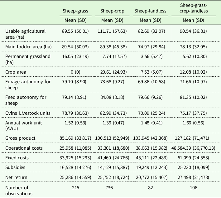
Notes SD: Std. dev.
The SERF method does not allow explicit treatments of panel data. Hence, in the present study, pooled data are used. It is worth noting that the SERF method accounts for individual effects given the fact that it does not use a fixed risk aversion coefficient for all the farms in the sample and that it estimates the CE for each farm according to the production systems. The SERF analysis can also be used to rank risky alternatives by type of decision makers (Richardson and Outlaw Reference Richardson and Outlaw2008). One way to account for time effects is to split the data into sub-periods and apply the SERF method per period. To avoid any ad hoc splitting, we need information on events that may cause structural breaks in the data. Since such information is not available in our dataset, we apply the SERF method to the pooled data over our study period. However, as indicated previously, to go a step further in our analysis, we use an econometric approach for examining time effects and the effects of other variables (including diversification patterns) on downside risk exposure. The econometric approach used can be seen as complementary to the SERF method.
Results and discussion
Diversification economies
We use the certainty equivalent (CE) values estimated using the SERF method to compute economies of diversification (ED) in the French sheep farms located in the Massif Central using equation (3). Such economies would exist if the CE value of the fully diversified farms is greater than the sum of the CE values of the partially diversified farms. The results concerning the existence of ED are shown in Figure 1.
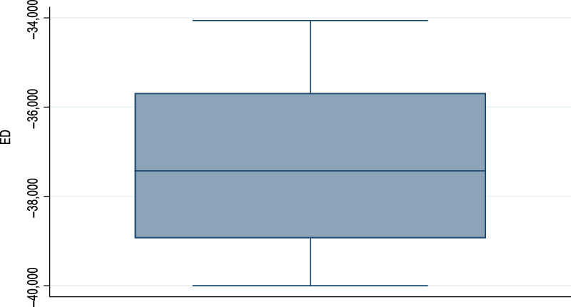
Figure 1. Economies (diseconomies) of diversification in French sheep farms.
Figure 1 indicates that all the values of the ED indicator are negative. This suggests that there are no economies of diversification in the sheep farming systems considered. That is, our results highlight the existence of diseconomies of diversification in our sheep farming systems. In order words, our results indicate that the fully diversified system considered does not generate more risk-adjusted returns (CE) than the partially diversified systems. To go a step further in our analysis, we also investigate the degree of diversification economies (DED) using equation (4), and the results are plotted in Figure 2.
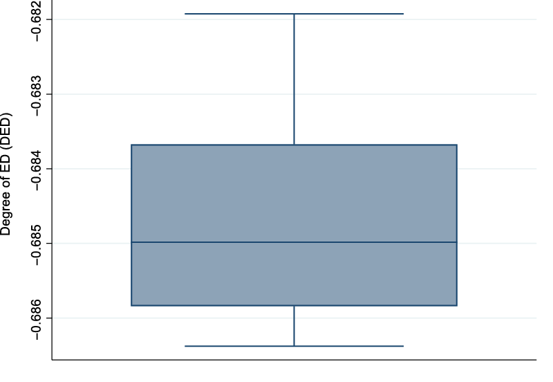
Figure 2. Degree of economies (diseconomies) of diversification (DED) in French sheep farms.
Figure 2 indicates that there is a relatively high degree of diseconomies of diversification in the sheep farming system considered. Indeed, all the values of the indicator of the degree of economies of diversification are negative and amount to -0.68 on average. This suggests that the fully diversified sheep system reaches only 32% of the risk-adjusted return (CE) generated by the partially diversified systems altogether. Using a quite different approach from ours, Fleming and Lien (Reference Fleming and Lien2009) showed that the existence of synergies (i.e., output complementarities) does not necessarily result in economic gains from diversification. Indeed, despite the existence of synergies, they found significant diseconomies for small-scale farming operations. Using the same approach as Fleming and Lien (Reference Fleming and Lien2009), Coelli and Fleming (Reference Coelli and Fleming2004) found weak evidence for diversification economies between subsistence food production, coffee, and cash food production, and diseconomies of diversification between coffee and cash food production. However, following Hajargasht, Coelli, and Rao (Reference Hajargasht, Coelli and Rao2008), Wimmer and Sauer (Reference Wimmer and Sauer2020) measure diversification economies as cost complementarities between individual outputs. They found that small dairy farms are more likely to benefit from diversification between milk and livestock production, while larger farms tend to benefit from diversification between milk and crop production. In sum, the existence of economies of diversification in mixed farms remains an open empirical question.
In Figure 3, we shed light on the sources of the observed diseconomies of diversification. Note that the sources of the observed diseconomies of diversification are not reported here as presented in equation (7), that is, we do not present directly $E{D_\pi }$
and
$E{D_\pi }$
and $E{D_R}$
. Indeed, for presentation convenience, we report in Figure 3
$E{D_R}$
. Indeed, for presentation convenience, we report in Figure 3 $E{D_\pi }/E\left[ \pi \right]$
and
$E{D_\pi }/E\left[ \pi \right]$
and $E{D_R}/R\left( \pi \right)$
. That is, we have scaled these measures in a similar way to the equation (4). Figure 3 shows that the mean return effect is negative while the risk effect is positive. The negative value for the mean return effect highlights that the average net return per family labor unit generated by the fully diversified system is lower than the one generated by the partially diversified systems altogether. The positive value of the risk effect indicates that the variance of the fully diversified system is lower than the one of the partially diversified systems altogether. Overall, the results from Figure 3 indicate that although the fully diversified system does not generate more returns than the partially diversified systems, it ensures more stable net returns. This suggests that farmers could consider the diversified system as a safer option for their farms (Sarwosri and Mußhoff Reference Sarwosri and Mußhoff2020) in the sense that it allows farmers to spread production and market risks (Villano, Asante, and Bravo-Ureta Reference Villano, Asante and Bravo-Ureta2019). These results are also in line with the portfolio theory, which suggests that diversified production systems should face lower risk (Markowitz Reference Markowitz1952 and Reference Markowitz1990; Paut, Sabatier, and Tchamitchian Reference Paut, Sabatier and Tchamitchian2019; Mosnier et al. Reference Mosnier, Benoit, Minviel and Veysset2021). They are also line with the idea that classical concepts (such as income maximization) that are often used to guide farm management are increasingly replaced by other concepts such as stability (Darnhofer et al. Reference Darnhofer, Bellon, Dedieu and Milestad2010; Astigarraga and Ingrand Reference Astigarraga and Ingrand2011).
$E{D_R}/R\left( \pi \right)$
. That is, we have scaled these measures in a similar way to the equation (4). Figure 3 shows that the mean return effect is negative while the risk effect is positive. The negative value for the mean return effect highlights that the average net return per family labor unit generated by the fully diversified system is lower than the one generated by the partially diversified systems altogether. The positive value of the risk effect indicates that the variance of the fully diversified system is lower than the one of the partially diversified systems altogether. Overall, the results from Figure 3 indicate that although the fully diversified system does not generate more returns than the partially diversified systems, it ensures more stable net returns. This suggests that farmers could consider the diversified system as a safer option for their farms (Sarwosri and Mußhoff Reference Sarwosri and Mußhoff2020) in the sense that it allows farmers to spread production and market risks (Villano, Asante, and Bravo-Ureta Reference Villano, Asante and Bravo-Ureta2019). These results are also in line with the portfolio theory, which suggests that diversified production systems should face lower risk (Markowitz Reference Markowitz1952 and Reference Markowitz1990; Paut, Sabatier, and Tchamitchian Reference Paut, Sabatier and Tchamitchian2019; Mosnier et al. Reference Mosnier, Benoit, Minviel and Veysset2021). They are also line with the idea that classical concepts (such as income maximization) that are often used to guide farm management are increasingly replaced by other concepts such as stability (Darnhofer et al. Reference Darnhofer, Bellon, Dedieu and Milestad2010; Astigarraga and Ingrand Reference Astigarraga and Ingrand2011).
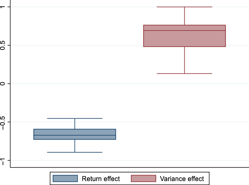
Figure 3. Sources of diversification economies.
Stochastic dominance analysis
This section presents the ranking of our four sheep farming systems using the SERF method, which is known as a more discriminating form of stochastic dominance analysis (Schenk et al. Reference Schenk, Hellegers, van Asseldonk and Davidson2014). However, for comparison purposes, CDF curves and the mean-standard deviation ranking for our sheep farming systems are depicted in Figures 4 and 5, respectively. Indeed, some general conclusions can be drawn from each of these methods.
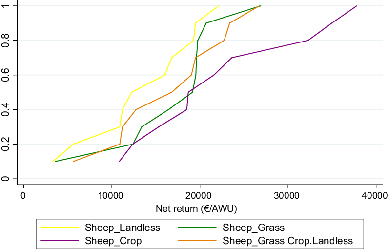
Figure 4. Cumulative distribution functions (CDFs) of the different sheep farming system (€/AWU).
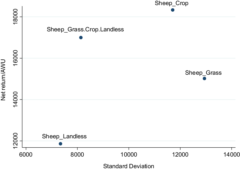
Figure 5. Mean-standard deviation plot of the four sheep farming systems.
The CDF curves show that the Sheep-Landless system is closest to the origin of the axes and does not intersect with the other sheep farming systems. This suggests that the Sheep-Landless system is dominated by the other systems. However, it is not feasible to rank the other systems using their CDFs since they intersect each other.
A general conclusion that can be drawn from Figure 5 is that the Sheep-Landless system has the lowest standard deviation for the net return per family labor unit. This suggests that this system could be a good strategy to mitigate economic risks. This could be explained by the off-land activities, which may be less sensitive to climatic context. In addition, in the Sheep-Landless system, the breeders work along integrated lines, mainly for poultry, that is, as subcontractors for agribusiness companies. In this system, the production is paid at a remunerative price even if the market conditions are unfavorable. Therefore, the market risk is shared between the breeders and the integrator. However, the Sheep-Landless system has also a disadvantage compared to the other systems: it has the lowest average net return per family labor unit. Among the farms studied, these farms have developed off-ground activities generally because they have a lack of land in relation to the available labor force; and sometimes because sheep profitability is too low. As our results show, the off-ground activities did not upset their economic results. This result is in line with Ripoll-Bosch et al. (Reference Ripoll-Bosch, Joy and Bernues2014) who found that production diversification might enhance farm flexibility but it is not necessarily related to economic performance. Similarly, Villagra et al. (Reference Villagra, Easdale, Giraudo and Bonvissuto2015) found that sheep represented the main source of income across different diversification schemes in Argentina, but it was not the most profitable livestock activity.
Note that Figure 5 also indicates that the Sheep-Grass (i.e., completely specialized) system exhibits the highest variability in the net return per family labor unit. This result highlights an interest in farms’ diversification (Chavas and Di Falco Reference Chavas and Di Falco2012). By considering relatively similar systems to ours, Prache, Caillat, and Lagriffoul (Reference Prache, Caillat and Lagriffoul2018) found that the system that exhibits the highest variability in terms of net returns over the past 10 years is the Sheep-Crop system. They argued that the Sheep-Crop system was very impacted by the climatic context and the fall of cereal prices. Our result is slightly different from the one of Prache, Caillat, and Lagriffoul (Reference Prache, Caillat and Lagriffoul2018) maybe because we consider the net return per family labor unit instead of the absolute value of the net return.
Nevertheless, from Figure 5, it appears that it is not feasible to rank our farming systems using the mean-standard deviation criterion. Indeed, while the Sheep-Landless system has the lowest mean and the lowest standard deviation, we cannot classify the other systems using both their means and their standard deviations. For instance, the Sheep-Crop system has the largest mean net return while the Sheep-Grass system has the largest standard deviation. Thus, with the mean-standard deviation criterion, none of the sheep farming systems has the largest mean net return and smallest standard deviation. In addition, none of them has the lowest average net return and the highest standard deviation. That is why their ranking under the mean-standard deviation criterion is difficult. However, it is worth noting that Figure 5 indicates that both the Sheep-Crop system and the fully diversified system would be preferred to the Sheep-Grass system by any risk-averse producer, since these systems generate higher net returns at lower risk (variance).
Figure 6 reports the results of the SERF method. These results are obtained by estimating the CE values by including the total subsidies received by farmers. Figure 7 reports the same results but without including the subsidies in the estimations. This may be useful for investigating the role of the subsidies in the ranking of the different systems.
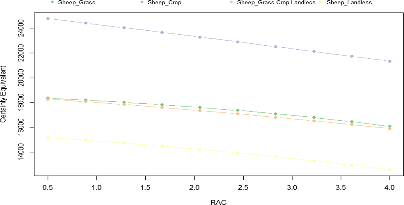
Figure 6. Certainty equivalent (CE) curves of net return (€/AWU) for the different sheep farming systems for a range of risk aversion coefficients (RAC).
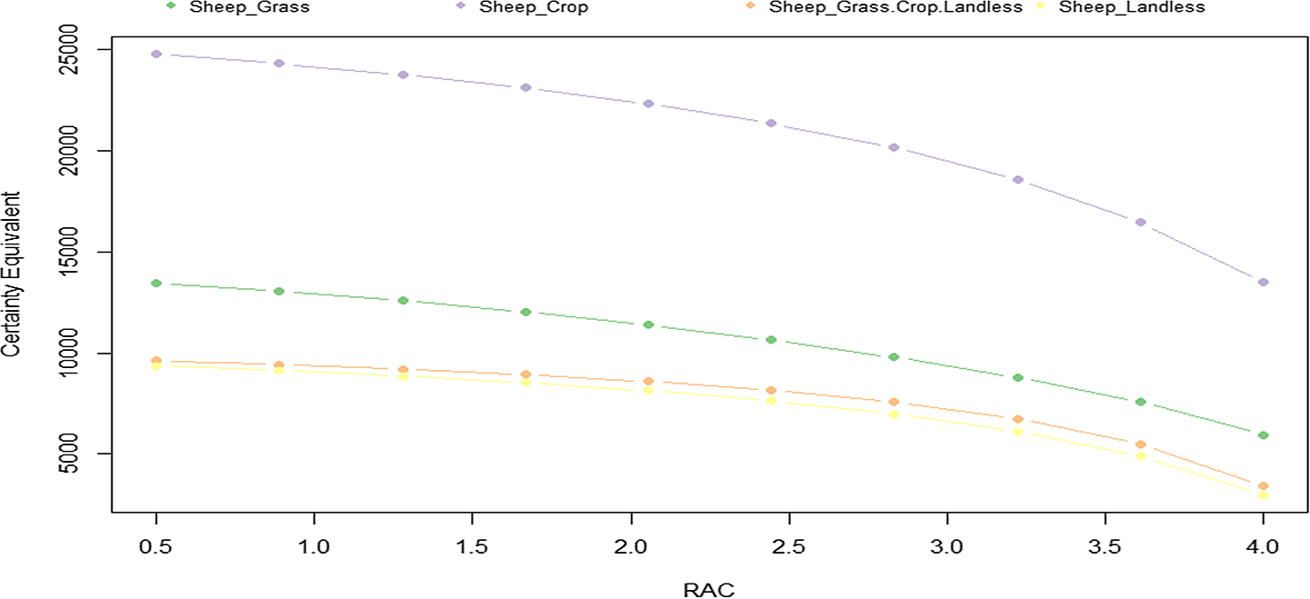
Figure 7. Certainty equivalent (CE) curves of net return (€/AWU) for the different sheep farming system (without subsidies) for a range of risk aversion coefficients (RAC).
The SERF analysis (Figure 6) confirms the fact that the Sheep-Landless system is dominated by the other ones in terms of risk-adjusted net return per family labor unit, as shown in the CDF curves (see Figure 4). Interestingly, the SERF analysis clarifies the rank of the other systems. Indeed, the SERF analysis (Figure 6) indicates that the Sheep-Crop system is the dominant alternative across all levels of risk aversion coefficients (RAC). Following Anderson and Dillon (Reference Anderson and Dillon1992), the relative RAC is equal to 0 for risk-neutral decision makers, 0.5 for slightly risk-averse decision makers, 1 for normally risk-averse decision makers, 2 for moderately risk-averse decision makers, and 4 for extremely risk-averse decision makers. By definition and as observed from Figures 6 and 7, the CEs decrease with an increase in the RAC. This means that the most risk-averse farmers have higher risk premiums than less risk-averse farmers. In this line, note that that the Sheep-Crop system exhibits the highest risk-adjusted return per family labor unit, regardless of the values of the RAC. This could be explained by the fact that this system benefits from larger structures (see Table 1) and that it is located in areas with relatively good agricultural potential (Benoit and Laignel Reference Benoit and Laignel2009; Venineaux-Delvalle et al. Reference Venineaux-Delvalle, Jousseins, Saget, Servière, Bataille, Cailleau and Bellet2017). Indeed, as industrial crops are more frequent in the rotations in the Sheep-Crop system, they provide access to various co-products to feed the sheep and the highest sheep feed autonomy (see Table 1). Another possible explanation is that the Sheep-Crop system facilitates the production of off-season lambs because it offers the possibility of feeding animals from co-products and crops produced on the farm (see Prache, Caillat, and Lagriffoul Reference Prache, Caillat and Lagriffoul2018), which may be valued by the market. Indeed, it is well known that from the economic law (supply and demand), off-season products can be better valued by the market. That is, they can be sold at more attractive prices, offsetting higher production costs.
The SERF analysis conducted without considering the subsidies received by farmers (Figure 7) provides a similar pattern. However, note that when the subsidies are taking into account (Figure 6), the Sheep-Grass and the fully diversified systems perform similarly; while without accounting for the subsidies (Figure 7), the Sheep-Landless and the completely diversified systems perform similarly. This may be understood in the sense that the performance of our fully diversified sheep systems relies mainly on the subsidies received by the farmers.
As previously mentioned, the SERF approach can be considered as a more discriminating form of the stochastic dominance analytical framework (Schenk et al. Reference Schenk, Hellegers, van Asseldonk and Davidson2014). In this respect, it is worth noting that the stochastic dominance analysis based on the SERF approach (Figures 6 and 7) provides more concrete evidence to explain the ranking of risky alternatives than the stochastic dominance analysis based on the CDF (Figure 4) (see also, Richardson and Outlaw Reference Richardson and Outlaw2008).
Econometric results on downside risk exposure
Prior to the econometric analysis, we test whether the farm income exhibited skewness. Using the test proposed by D’Agostino, Balanger, and D’Agostino (Reference D’Agostino, Balanger and D’Agostino1990), we find that the skewness is statistically different from zero, with a p-value of 0.000. We, therefore, reject the null hypothesis of normality due to skewness at the 1% significance level. Table 2 reports the econometric results on the effects of the diversified systems on downside risk exposure measured through the third moment (the skewness) of the farm income. Recall that an increase in the skewness means that downside risk exposure decreases, that is, the probability of failure decreases (Di Falco and Chavas Reference Di Falco and Chavas2009). This suggests that variables that are positively associated with the skewness involve a reduction in the downside risk exposure. Most of the estimated coefficients shown in Table 2 are statistically different from zero at the 5% significance level. This indicates that most of the explanatory variables used have significant effects on the downside risk exposure. Except for farm capital, all the significant variables have a positive effect on skewness, meaning that they can reduce farm exposure to downside risk.
Table 2. Econometric estimates for the skewness of farm income
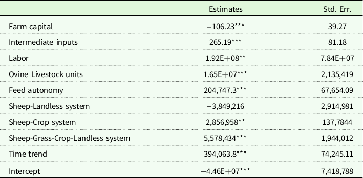
The asterisks ***, **, and * indicate significance at the 1, 5, and 10% levels, respectively.
More specifically, we find that farm capital has a statistically significant and negative effect on skewness. This result suggests that the existing capital stock tends to increase downside risk by causing the collapse of farmers’ net income under unfavorable production or market conditions. The coefficients of the intermediate inputs and the number of livestock units are positively related to the skewness, suggesting that these variables appear to be downside risk decreasing. This may be due to the fact that these variables are proportional to the production levels. The findings related to capital and intermediate input effects are consistent with Di Falco and Veronesi (Reference Di Falco and Veronesi2014), while the findings on livestock units are consistent with Finger et al. (Reference Finger, Dalhaus, Allendorf and Hirsch2018). We find that labor has a significant positive effect on skewness. This implies that the availability of labor can help farmers to manage downside risk by reducing the likelihood of farm activities disruption. Similar results can be found in Bozzola and Finger (Reference Bozzola and Finger2021). The variable feed autonomy is positively related to the skewness, suggesting that feed autonomy contributes to the reduction of downside risk exposure by lowering farm production costs. This could also be understood in the sense that feed autonomy allows farmers to avoid production failure under unfavorable input market conditions. The positive and significant coefficient of the time trend suggests that downside risk exposure decreases with time. Note that the coefficient of the Sheep-Landless system is not statistically significant. Thus, our estimates do not provide enough evidence on the potential of this system for managing downside risk exposure.
The coefficients associated with the Sheep-Crop system and the fully diversified system (Sheep-Grass-Crop-Landless) are positive and significant. This suggests that compared to the Sheep-Grass system (the reference category), the Sheep-Crop system and the fully diversified system can help farmers to reduce exposure to downside risk. Such results are consistent with many studies showing that farm diversification is a production strategy that allows farmers to manage exposure to downside risk (Kim and Chavas Reference Kim and Chavas2003; Di Falco and Chavas Reference Di Falco and Chavas2009). The coefficient of the Sheep-Crop system is significant at the 5% level while the coefficient of the fully diversified system is significant at the 1% level. These results indicate that the fully diversified system can be very effective in reducing exposure to downside risk (Di Falco and Chavas Reference Di Falco and Chavas2006). These results could also be interpreted in terms of economic resilience. Indeed, resilience can be defined as the capacity of a system to withstand external shocks without catastrophic consequences (Holling Reference Holling1973). In this respect, our results indicate that diversification increases the ability of the production systems to absorb downside shocks (Di Falco and Chavas Reference Di Falco and Chavas2006). In this line, our results suggest that diversification strategies are successful risk management strategies that make farms more resilient to unfavorable production or market conditions. Our results also suggest that the fully diversified system would be the most resilient (Di Falco and Chavas Reference Di Falco and Chavas2006).
Concluding remarks
This study investigates the existence and the components of economies of diversification in sheep farming systems in France. It also identifies stochastic dominant mixtures of sheep farming activities in terms of risk-adjusted net returns. To examine the economies of diversification, we compare partially diversified systems (Sheep-Grass, Sheep-Crop, and Sheep-Landless) with fully diversified systems (Sheep-Grass-Crop-Landless) in terms of certainty equivalents of their net returns per family labor unit. The certainty equivalent of the net return is a risk-adjusted measure that makes it possible to integrate two economic rationales for production diversification: risk-reducing effect and scope economies effect. To identify the stochastic dominant mixtures of sheep farming activities, we use the stochastic efficiency with respect to a function (SERF) analysis, which is also known as a generalized method of stochastic dominance analysis.
Our empirical analysis is undertaken on an unbalanced panel of 1,139 observations from 134 mixed sheep farms located in an area of the Center of France, namely the Massif Central, over the period 1987 to 2017. The Massif Central is classified in the so-called Less Favored Agricultural Area (LFA). An advantage of sheep farming is that sheep are well suited to valorize LFA. In spite of that, sheep farmers in the Massif Central have to face risk and uncertainty due to unforeseen climate conditions, sanitary issues, and price volatility. In this context, our analysis may provide relevant information for designing/selecting mixtures of farming activities that allow farmers to have greater risk-adjusted returns, or to reduce their economic risk. This may be insightful for producers who think about changing their production mix in order to continue to valorize the potentialities of their territory.
The results indicate that there are no economies of diversification in the sheep farming systems considered. That is, we find that the fully diversified system considered does not generate more risk-adjusted returns (CE) per family labor unit than the partially diversified systems. In addition, we find that all the values of the indicator of the degree of economies of diversification are negative and amount to -0.685 on average. This suggests a relatively high degree of diseconomies of diversification in the sense that the completely diversified sheep system reaches only 31.5% of the risk-adjusted returns (CE) generated by the partially diversified systems altogether. Regarding the sources of the observed diseconomies of diversification, we find that the average net return per family labor unit generated by the fully diversified system is lower than the one generated by the partially diversified systems altogether, while the variance component of the fully diversified system is lower than the one of the partially diversified systems. This suggests that the observed diseconomies of diversification are mainly due to the mean return effect. That is, the diversified system does not generate more returns than the partially diversified systems, but it ensures more stable returns. However, since the variance does not distinguish between upside and downside shocks (i.e., good and bad events), special attention has been devoted to the effects of diversification on downside risk exposure. In this respect, our results indicate that the Sheep-Crop and the fully diversified systems (Sheep-Grass-Crop-Landless) considered can be effective in reducing exposure to downside risk.
The dominance stochastic analysis conducted using the SERF method reveals that the dominant system in terms of risk-adjusted returns is the Sheep-Crop one. This may be due to the fact that these systems: (i) benefit from more attractive prices (for off-season products); and (ii) concern large farms located in areas favorable to cash crops. We also find that the returns of the Sheep-Landless system exhibit the lowest variability, while the ones of the fully specialized (Sheep-Grass) system exhibit the largest variability. Note also that the variability of the returns of the fully specialized (Sheep-Grass) system is rather close to that of the Sheep-Crop system (Figure 5). We recognize these differences may reflect the heterogeneity of the diversification strategies of farmers. For instance, we admit that each farmer trades off risk and returns at a personal (or individual) rate. In addition, diversification decisions could also be related, among other things, to soil quality, microclimate, historical context, territorial norms and constraints, and soil conservation strategies. It could also depend on: (a) individual circumstances; (b) resource availability (e.g., workforce, land, fixed capital); (c) farmers’ skills; (d) farmers’ desire to contribute to social and environmental objectives; (e) abilities; (f) incentives and existence of marketing channels (or market opportunity); and (g) extension service for a given production (see also, McNally Reference McNally2001; Meert et al. Reference Meert, Van Huylenbroeck, Vernimmen, Bourgeois and Van Hecke2005; Leck, Evans, and Upton Reference Leck, Evans and Upton2014; McFadden and Gorman Reference McFadden and Gorman2016; Suess-Reyes and Fuetsch Reference Suess-Reyes and Fuetsch2016; Morris, Henley, and Dowell Reference Morris, Henley and Dowell2017). For instance, it is recognized that larger farms and farms with greater assets are more likely to diversify their production activities (McInerney and Turner Reference McInerney and Turner1991; Ilbery Reference Ilbery1991; McNally Reference McNally2001).
In the same vein, the different systems could co-exist given specific farm characteristics and many contextual drivers. In this line, Villano, Fleming, and Fleming (Reference Villano, Fleming and Fleming2010) argued that the choice of diversification may be a function of a number of factors outside the farmer’s control. In addition, previous studies (e.g., McNally Reference McNally2001; Pardos et al. Reference Pardos, Maza, Fantova and Sepúlveda2008; Maye, Ilbery, and Watts Reference Maye, Ilbery and Watts2009; Hansson et al. Reference Hansson, Ferguson, Olofsson and Rantamaki-Lahtinen2013; Morris, Henley, and Dowell Reference Morris, Henley and Dowell2017) found significant heterogeneity among farmers in their motives for diversifying their production activities. Using econometrics techniques, the effects of the diversified system considered on downside risk exposure were examined by controlling for some of the above factors (available in our data set). However, further research on the production capacities of the farms, their characteristics, and their contextual drivers could provide additional information on their diversification strategies. As such, it would be difficult to prescribe a specific sheep farming system to farmers from our results.
However, from an economic standpoint, an important goal of farm diversification is to find combinations of farming activities that provide the best compromise between the farm return and its variability. In addition, as our results show, diversified production systems could also be driven by their ability to reduce downside risk exposure. In this respect, we believe that, in addition to producers who think about changing their production mix, our results could provide insights to policy makers and extension professionals. They can inform policy-makers’ decisions on the components of the observed diseconomies of diversification in mixed sheep farms in the Massif Central. Extension professionals can distribute the information from our results to help farmers to make better diversification decisions.
Acknowledgements
The authors would like to thank the editor and the anonymous reviewers for their helpful and relevant suggestions that helped us to improve significantly the quality of this article.
Funding statement
This research received no specific grant from any funding agency, commercial or not-for-profit sectors.
Conflicts of interest
The authors declare no conflict of interest.
Data availability statement
Replication materials are available by request to the authors.
Appendix
Appendix A. The livestock in the Massif Central (for all farms)

Sources: Own elaboration with data from SIDAM (2020)
Appendix B. Average price (weighted by regions) of French sheep (lamb)
Sources: Own elaboration with data from FranceAgriMer


 Open access