1. Introduction
Controlling tropical deforestation is critical to reducing global greenhouse gas emissions, particularly because a hectare of tropical forest has four times the $CO_2$ absorption value compared to other forests (Taye et al., Reference Taye, Folkersen, Fleming, Buckwell, Mackey, Diwakar, Le, Hasan and Saint Ange2021). The COVID-19 pandemic and the resulting government responses led to a sudden halt in social and economic activity worldwide. While this slowdown had positive environmental effects, such as reductions in air pollution and wildlife returning to urban areas (Cicala et al., Reference Cicala, Holland, Mansur, Muller and Yates2020; López-Feldman et al., Reference López-Feldman, Chávez, Vélez, Bejarano, Chimeli, Féres, Robalino, Salcedo and Viteri2020; Brock et al., Reference Brock, Doremus and Li2021), the pandemic's impact on deforestation outside of cities has not yet been fully studied. In this paper, we aim to address this gap by using micro-data to analyze the impact of COVID-19 lockdowns on deforestation.
The pandemic and associated lockdown restrictions have the potential to affect deforestation through various channels. On the one hand, deforestation could decrease if loggers comply with government lockdown orders and if the demand for land and timber decreases due to the global economic recession. It's worth noting that foreign demand for wood is significant, accounting for 42 per cent of the total forestland harvested area (Arto et al., Reference Arto, Cazcarro, Garmendia, Ruiz and Sanz2022).Footnote 1 On the other hand, deforestation may increase due to at least two reasons. First, the reduction in alternative income sources resulting from lockdowns may push people towards forest-clearing activities (Ferraro and Simorangkir, Reference Ferraro and Simorangkir2020; Jayachandran, Reference Jayachandran2021). Second, the lockdowns could be stricter for forest departments than for farmers and loggers. Global deforestation might be unaffected by a combination of these channels in different regions. Given all these theoretical possibilities, we turn to the data to study this issue empirically.
We combine bi-weekly (every two weeks) data from 70 countries covering the entire world's tropical forests with the dates each country introduced lockdown restrictions. The data on vegetation cover change alerts is from Hansen et al. (Reference Hansen, Krylov, Tyukavina, Potapov, Turubanova, Zutta, Ifo, Margono, Stolle and Moore2016). Since this data does not differentiate between vegetation changes in natural forests vs. plantations (Fergusson et al., Reference Fergusson, Saavedra and Vargas2020), we restrict the alerts to areas of primary forest. Thus, we refer to Hansen et al. (Reference Hansen, Krylov, Tyukavina, Potapov, Turubanova, Zutta, Ifo, Margono, Stolle and Moore2016) alerts that are restricted to forests in this way as “deforestation alerts”. The start dates for the lockdown orders in each country come from the Oxford COVID-19 policy tracker (Hale et al., Reference Hale, Webster, Petherick, Phillips and Kira2020). We obtain the share of gross domestic product (GDP) lockdown-vulnerable from United Nations (United Nations Department of Economic and Social Affairs, 2020).
We use difference-in-differences regressions to study the lockdowns’ effect on deforestation (Greenstone and Gayer, Reference Greenstone and Gayer2009. The empirical strategy compares deforestation across countries before and after the beginning of each country's lockdown. We use municipality fixed effects to control for time-invariant characteristics that make an area more or less vulnerable to deforestation, such as the presence of roads and rivers, the slope of the terrain, and whether the forest is in a protected natural area (Deng et al., Reference Deng, Huang, Uchida, Rozelle and Gibson2011; Busch and Ferretti-Gallon, Reference Busch and Ferretti-Gallon2017). We also use region times bi-week fixed effects to account for common shocks to an area in a given two-week interval. For example, COVID-19 cases and weather conditions. Ultimately, this allows us to compare neighboring municipalities in different countries with different lockdown start dates, in the spirit of Burgess et al. (Reference Burgess, Costa and Olken2018). Given the variation in lockdown dates, the traditional two-way fixed effects estimator might be biased (Marcus and Sant'Anna, Reference Marcus and Sant'Anna2021; Goodman-Bacon, Reference Goodman-Bacon2018); therefore we also use the estimator of Callaway and Sant'Anna (Reference Callaway and Sant'Anna2021). Although we include municipality and region times bi-week fixed effects, the estimated coefficient is a bundle of the lockdown effect, the COVID-19 health shock, and the economic slowdown. We also analyze heterogeneous effects of lockdowns in deforestation using within country variation in Colombia.
We find that the average effect of lockdowns on deforestation is not distinguishable from zero. This result is in line with the conclusions of other papers that COVID-19 did not affect countries’ pre-existing deforestation trends (Wunder et al., Reference Wunder, Kaimowitz, Jensen and Feder2021; Céspedes et al., Reference Céspedes, Sylvester, Pérez-Marulanda, Paz-Garcia, Reymondin, Khodadadi and Castro-Nunez2023). However, there are two important dimensions of heterogeneity. First, there is differentially higher deforestation in countries with a higher share of lockdown-vulnerable GDP. If alternative income sources are more likely to dry up, inhabitants turn to deforestation. Second, deforestation is reduced in countries with effective governments because they can enforce lockdown restrictions. Two additional pieces of evidence support these heterogeneous results. First, we likewise observe a smaller reduction in mobility in countries with a higher share of lockdown-vulnerable GDP. Second, we also find that, within the country of Colombia, there is more deforestation in municipalities with a higher share of vulnerable GDP and more deforestation reductions in municipalities with better governance. The results are robust to different lockdown definitions and functional form specifications.
This study is the first to use microdata to examine the effect of the COVID-19 pandemic response on global deforestation. López-Feldman et al. (Reference López-Feldman, Chávez, Vélez, Bejarano, Chimeli, Féres, Robalino, Salcedo and Viteri2020) discussed the possible mechanisms through which the pandemic might affect deforestation. Previous studies have examined the opposite relationship: the effect of environmental conditions on health, including the impact of UV radiation on COVID-19 transmission (Carleton et al., Reference Carleton, Cornetet, Huybers, Meng and Proctor2020), and forest loss on malaria and infectious diseases (Keesing et al., Reference Keesing, Belden, Daszak, Dobson, Harvell and Holt2010; Garg, Reference Garg2019). Numerous papers have used yearly satellite data to conduct regression analyses of deforestation before (Jayachandran et al., Reference Jayachandran, De Laat, Lambin, Stanton, Audy and Thomas2015; Berazneva and Byker, Reference Berazneva and Byker2017; Blackman et al., Reference Blackman, Goff and Planter2018; Jung and Polasky, Reference Jung and Polasky2018). However, to the best of our knowledge, this is the first study taking advantage of the bi-weekly alerts.
More broadly, this paper contributes to the literature on whether deforestation can be prevented with economic incentives or government commitments. Our results show the importance of alternative economic sources, in line with the results of Sims and Alix-Garcia (Reference Sims and Alix-Garcia2017) and Jayachandran et al. (Reference Jayachandran, De Laat, Lambin, Stanton, Audy and Thomas2017). The results also demonstrate that policies to reduce deforestation are successful when the government is effective. This result aligns with the success of previous Brazilian policies designed to reduce deforestation (Juliano et al., Reference Juliano, Gandour and Rocha2015; Burgess et al., Reference Burgess, Costa and Olken2018).
2. Data and estimating equations
2.1 Lockdowns and socio-economic data
The COVID-19 pandemic caused around 7 million deaths worldwide (Our World in Data, 2020). Some countries enacted minimum restrictions, while others imposed strict measures. Hale et al. (Reference Hale, Webster, Petherick, Phillips and Kira2020) tracks each country's policies in categories such as containment and closure, economic response, and health systems. The main specification uses the date when workplace closure orders started in each country. Specifically, we construct a dummy “Lockdown=1” when Hale et al. (Reference Hale, Webster, Petherick, Phillips and Kira2020) indicates the government “requires closing (or working from home) for some sectors or categories of workers” or “requires closing (or working from home) for all-but-essential workplaces (e.g., grocery stores, doctors)”; and the dummy “Lockdown=0” when no measures or closing is recommended but not required. As a robustness check, we also use the date when stay-at-home orders were in place or restrictions on internal movement began. We also determine inhabitants’ level of compliance with the lockdown orders using data from Google's mobility reports (Google LLC, 2020).
Table 1, panel A presents summary statistics at the country level for the 70 countries included in the analysis. On average, the countries introduced restrictions in bi-week 6.7 of the year 2020, which is around March 31. Most countries had not ended the restrictions at the end of the study period (July 12), so there are only 21 observations for the bi-week when the lockdown ended. See figure A1(A) for the evolution of the percentage of countries under lockdown by bi-week.
Table 1. Summary statistics
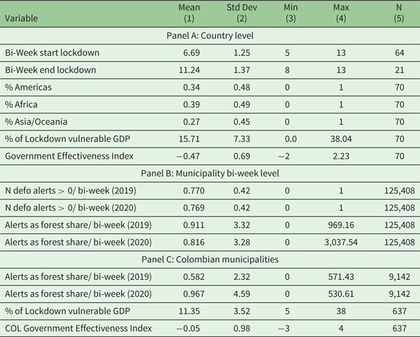
Notes: Panel (A) presents data on the countries in the sample used for the regression analysis. Column (1) is the mean, and column (2) the standard deviation. Columns (3) and (4) are the minimum and maximum values of the variable for a country, respectively. There are fewer observations for the lockdown start/end bi-week because some countries did not impose workplace closure restrictions or had not ended restrictions by July 12, 2020. Panel (B) presents the deforestation data at the municipality bi-week level, the level used in the regression analysis. Alerts as forest share were calculated as the number of pixels with deforestation alerts per 10,000 forest pixels. Panel (C) is restricted to Colombian municipalities.
We study the heterogeneous effects of the lockdown orders by the percentage of a country's gross domestic product (GDP) vulnerable to lockdown restrictions. For lockdown-vulnerable GDP, we take as a proxy the share of wholesale, retail trade, restaurants, and hotels because these sectors depend on lockdown-restricted human interactions. We use data from United Nations Department of Economic and Social Affairs (2020).Footnote 2 Table 1 shows that the share of vulnerable GDP varies from 0 to 70 per cent with a mean of 46 per cent. This country proxy is not perfect because it is influenced by cities not included in the analysis. In cities, services jobs are prone to remote working, while in forested municipalities, they represent wholesale and retail trade (including hotels and restaurants) that we want to capture. We explore the economic channel further using municipality-level data for Colombia from the National Planning Department (DNP, 2018). We obtain the share of each municipality's GDP attributed to restaurants, hotels, and sales. These sectors were largely affected by the lockdowns, so this information allows us to study the economic channel of the lockdowns’ effect on deforestation.
We use an index of government effectiveness provided by the World Bank (2020) to measure the likelihood of compliance with lockdown orders. This index captures perceptions of the quality of the civil service and the quality of policy formulation and implementation. It is standardized to have a global mean of 0 and a standard deviation of 1. The global index varies from approximately $-2.5$ to 2.5 (higher values indicate better governance). Colombia, the country we use for the within-country analysis, has a government effectiveness of $-0.09$
 . For Colombian municipalities, we use the effectiveness index constructed by DNP (2018). We standardized the index to make the Colombian estimate comparable to the global one.
Around a third of the countries in the sample are in the Americas, 39 per cent in Africa, and 27 per cent in Asia-Oceania. We obtained the map of the administrative divisions of each country from University of California Davis (2018). For most countries, we use the second administrative division, equivalent to counties and municipalities. But some small countries have only one level of division, the equivalent of states. See table B1 in the online appendix for details of each country. We measure the municipality's remoteness as the distance to the country's capital. We standardized the distance within each country to have a mean of 0 and a standard deviation of 1.
To study compliance with lockdown restrictions, we use data from Google's mobility report (Google LLC, 2020). This data uses anonymized phone locations and time patterns to identify aggregate mobility compared to a pre-lockdown day.Footnote 3 We use the percentage change in mobility to workplaces, measured by the change in total visitors.
2.2 Deforestation
Data for vegetation cover change alerts was obtained from Hansen et al. (Reference Hansen, Krylov, Tyukavina, Potapov, Turubanova, Zutta, Ifo, Margono, Stolle and Moore2016) for every bi-week from January 1 to July 12 for 2019 and 2020.Footnote 4 This data is constructed by analyzing satellite imagery and searching for disturbances in vegetation cover. The alerts are reported in squared pixels of $0.00025^{\circ }$ , approximately 28 meters at the equator. We aggregate the data at the municipality bi-week level and calculate the number of deforestation alerts per 10,000 forest pixels. Although the share of forest pixels that are deforested is our main dependent variable, we also use the number of alerts as a robustness check, and the results remain the same.
There are three main issues with the alerts data.Footnote 5 First, it does not differentiate between the deforestation of natural forests and tree logging in plantations (Fergusson et al., Reference Fergusson, Saavedra and Vargas2020). Second, the date an alert is reported is not necessarily the date the deforestation happened because clouds might obstruct immediate detection. Finally, false positives are removed if not confirmed in a follow-up image in the next six months. To address the first issue, we restrict the alerts to areas classified as primary forests by Turubanova et al. (Reference Turubanova, Potapov, Tyukavina and Hansen2018), and call them deforestation alerts. To address the other two issues, we include region bi-week fixed effects to absorb under/over-reporting of alerts in a given area. An alternative way to deal with the third issue is to study whether the results vary based on the data's processing date. For example, instead of using the 2019 alert data as of 2020, where most alerts have been purged, we can use the 2019 alerts as of July 2019. This criteria will leave both years with a similar lag of processing noise.
Figure 1(A) presents the forest areas of the world in green and the gray “pathrow” squares for the areas included in the alerts. The Hansen et al. (Reference Hansen, Krylov, Tyukavina, Potapov, Turubanova, Zutta, Ifo, Margono, Stolle and Moore2016) data is for humid tropical forests, so the forests of Canada, Russia, and Europe are not included in this study. As the alerts’ data comes in squares of neighboring regions, we will use these squares in one of the estimation strategies to compare lockdown areas within neighboring regions.
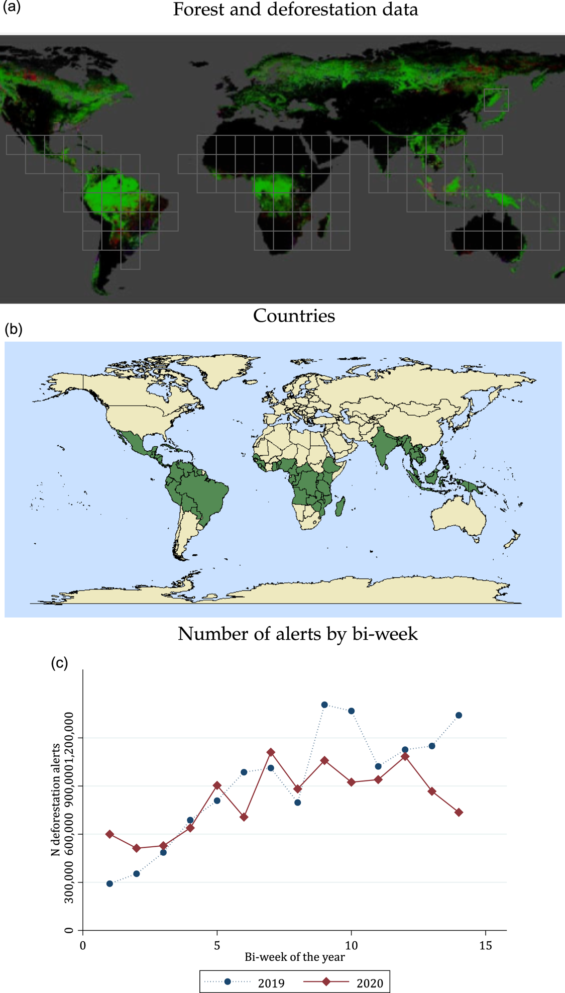
Figure 1. Deforestation alerts data. (A) Forest and deforestation data, (B) Countries, (C) Number of alerts by bi-week. Notes: Panel (A) shows forests in green; and squares areas with deforestation alerts in gray. Panel (B) shows in dark green countries included in the regression because they have data on deforestation alerts and lockdown information. Panel (C) presents the total number of deforestation alerts in 2019 (blue circles) and 2020 (red diamonds). The x-axis is the bi-week of the respective year, and the y-axis the number of deforestation alerts. Map source: http://glad-forest-alert.appspot.com/.
Figure 1(B) presents the map of countries with deforestation alert data and lockdown information, which are consequently included in the analysis. The largest countries in the sample are Brazil, the Democratic Republic of the Congo, and Indonesia.Footnote 6
Figure 1(C) presents the total number of tropical deforestation alerts in all countries in the sample by bi-week. Globally there are around 800,000 deforestation alerts each bi-week. There is no change around bi-week 7 (end of March), when most countries introduced lockdown orders. Panel B of table 1 presents summary statistics at the municipality bi-week level, the dependent variable of the main regressions. On average, around 77 per cent of the municipality bi-week observations include a deforestation alert, equivalent to around one alert per 10,000 pixels (0.01 per cent) of the forest area. Note that only municipalities with primary forests are included.
2.3 Estimating equations
We estimate whether deforestation was reduced during COVID-19 lockdowns using difference-in-differences strategies. That is, we compare deforestation before and after the lockdowns were imposed in countries under lockdown, to countries that did not have a lockdown that bi-week. We have data at the municipality bi-week level for 8965 municipalities with forests in 70 tropical countries. The primary sample comprises 14 bi-weeks from January-July 2020, the first year of the pandemic. We use data for January-July 2019 for a triple difference-in-differences strategy. We estimate equation (1):

where $Y_{mcsnw}$ is a measure of deforestation in municipality $m$
 , country $c$
 , deforestation data square $s$
 , continent $n$
 , in bi-week $w$
 . In the main specifications, we use the number of pixels with deforestation alerts per 10,000 forest pixels. $Lockdown_{cw}$
 indicates whether country $c$
 was under lockdown in bi-week $w$
 . $\gamma _m$
 are municipality fixed effects to capture time-invariant characteristics that affect deforestation, like distance to the country's capital, the presence of roads and rivers, the terrain's slope, and whether the forest is in a protected natural area (Deng et al., Reference Deng, Huang, Uchida, Rozelle and Gibson2011; Busch and Ferretti-Gallon, Reference Busch and Ferretti-Gallon2017). $\gamma _{nw}$
 are continent-bi-week fixed effects to control for shocks like COVID-19 cases and the weather. We weigh the observations according to the area of primary forest in the municipality. Consequently, we estimate the effect on the average forest pixel. Finally, $\varepsilon _{m,sw}$
 is an error term that we cluster two ways: at the municipality level and the data square bi-week level. As mentioned in the previous sub-section, the deforestation data is processed by squares of satellite images; therefore, observations for municipalities in the same data square are correlated due to errors in each satellite image. The identification for $\beta _1$
 comes from differential deforestation rates for municipalities under lockdown compared to those in the same continent that were not under lockdown.
Equation (1) assumes a common shock for all countries in the same continent bi-week. However, there is considerable variation in COVID-19 cases and the weather within the same continent. Consequently, we exploit the satellite image square $s$ to which each municipality belongs. Figure 2 presents an example of two different deforestation data squares that cover Colombian municipalities. The square on the left covers the southern border of Colombia with Ecuador, Peru, and Brazil. The square on the right includes the eastern border of Colombia with Venezuela, Brazil, and Guyana. The square-bi-week fixed effects ($\gamma _{sw}$
 ) in equation (2) absorb any common shock to the forest in each square during a given bi-week. If the square covers many countries, we can compare deforestation in municipalities of countries with different lockdown timings. For example, as Colombia started its lockdown on bi-week seven and Brazil on bi-week nine, our empirical strategy compares differential deforestation rates in those two bi-weeks in the border Amazon municipalities in the same square. The identification for $\beta _2$
 in equation (2) comes from differential deforestation rates in municipalities under lockdown compared to those in nearby countries that were not locked down. Note that if a square covers only one country, the square bi-week fixed effect will absorb the lockdown effect in that country.

One possible concern with the two specifications described above is that the estimated coefficients ($\beta _1$ , $\beta _2$
 ) might confound the lockdown effect with differences in seasonal variation across countries. We use two approaches to address this concern. First, we conduct a placebo estimation of equation (2) using 2019 data and assuming lockdowns happened in the same bi-weeks as in 2020. Second, we simultaneously use 2020 and 2019 deforestation data in a triple difference-in-differences specification. This specification allows us to use country bi-week of the year fixed effects to capture specific country seasonality. Specifically, we estimate

$Y_{mcswy}$ is a measure of deforestation in municipality $m$
 , country $c$
 , square $s$
 , in bi-week $w$
 of year $y$
 . $Lockdown_{cwy}$
 is an indicator for whether country $c$
 was under lockdown in bi-week $w$
 of year $y$
 , that is, only for observations in 2020 ($y=2020$
 ). $\gamma _{cy}$
 are country-year fixed effects, $\gamma _{cw}$
 are country bi-week of the year fixed effects, and $\gamma _{swy}$
 square bi-week year fixed effects. The identification for $\beta _3$
 comes from differential deforestation rates in municipalities under lockdown compared to municipalities in the same square that were not under lockdown, net of deforestation differences the year before.
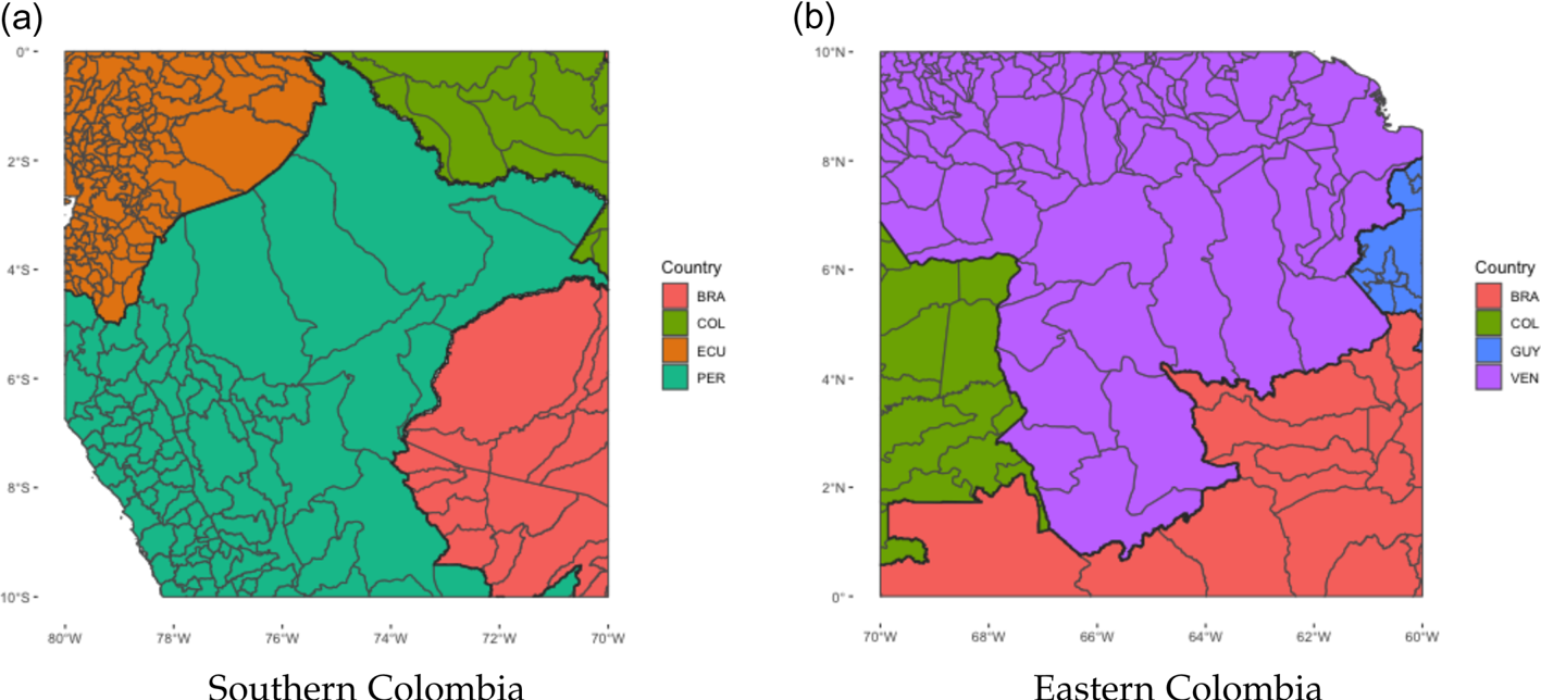
Figure 2. Example of deforestation data squares covering multiple countries. (A) Southern Colombia, (B) Eastern Colombia. Notes: This figure presents two squares in which deforestation alerts are reported. Using data square bi-week fixed effects absorbs any common shock to the area, such as the weather or COVID-19 cases. Thus, we can estimate the effect of differential lockdown timings across neighboring countries on equation (2).
3. Results
Table 2 presents the results of estimating equations (1)–(3). Columns (1) and (2) present the results of estimating equation (1), with country and municipality fixed effects, respectively. In both cases, the estimated effect is not statistically different from zero. That is, deforestation did not change differentially after the start of the lockdowns. Column (3) presents the results of estimating equation (2), and it also shows no evidence of differential changes in deforestation when lockdowns started. Column (4) estimates the placebo test: equation (2) using data from 2019. Columns (5) and (6) also show no changes in deforestation with the lockdowns when using the triple difference-in-differences strategies.
Table 2. Main results
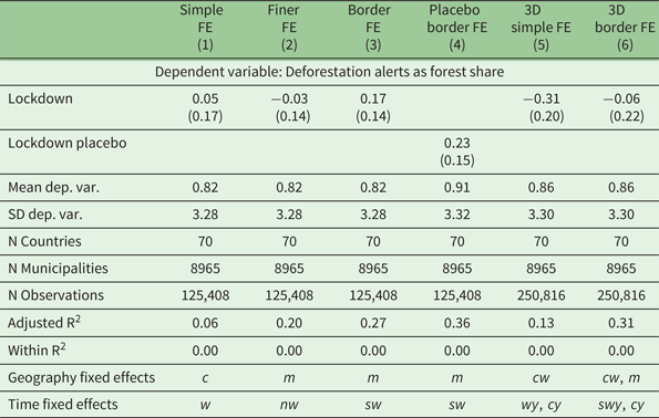
Notes: Alerts as forest share calculated as the number of pixels with deforestation alerts per 10,000 forest pixels. The fixed effects notation represent bi-week $w$ , year $y$
 , municipality $m$
 , country $c$
 , square $s$
 and continent $n$
 . Columns (1)–(2) report the coefficients obtained from estimating equation (1) with different fixed effects, and columns (3)–(4) the results of estimating equation (2). Column (3) uses 2020 data and column (4) assumes the lockdowns happened in 2019 for the placebo estimation. Finally, columns (5) and (6) present the coefficients from estimating equation (3). Clustered standard errors at the municipality and square bi-week level are in parentheses.
Figure 3 presents the results of estimating the dynamic difference-in-differences version of equation (1). There are no statistically significant differences before the start of the lockdown, which provides support for the parallel trends assumption. After the start of the lockdown, there are also no statistically significant differences, as shown in average in table 2. The coefficient of bi-week $3$ is significant in figure 3, but is no longer statistically significant when we do the analogous graphs for equations (2) and (3) (appendix figure A2, panels C and D respectively).
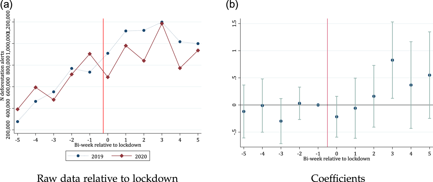
Figure 3. Dynamic specification. (A) Raw data relative to lockdown, (B) Coefficients. Notes: Panel (A) presents raw data relative to lockdown date. Panel (B) presents the dynamic coefficients obtained from the estimation of equation (1) together with 95 per cent confidence intervals. The figures present the window 5 bi-weeks before and 5 bi-weeks after the start of lockdown restrictions.
In table 3, we analyze the heterogeneous effects of lockdowns on deforestation. Column (1) repeats the results of column (3), table 2 for comparison. In column (2), we interact the lockdown dummy with the percentage of lockdown-vulnerable GDP. Deforestation is reduced by 1.01 alerts per 10,000 forest pixels when a country is under lockdown and has a small percentage of lockdown-vulnerable GDP. We can reject that both coefficients are zero at the 5 per cent level, using the F-statistic testing the joint significance of the lockdown and the interacted coefficient. However, when a country has a larger share of vulnerable GDP, the reduction in deforestation is smaller and can even increase deforestation. In column (3), we study heterogeneity by the government effectiveness index. We find that deforestation was reduced during lockdowns in countries with good governance. Column (4) interacts the lockdown dummy with the municipality's relative remoteness. The coefficient is not statistically different from zero. In column (5), we interact the lockdown indicator with the percentage of primary sector GDP (agriculture, hunting, forestry, fishing). The coefficient is only significant at the 10 per cent level and indicates lower deforestation for lockdown countries relying more on the primary sector. As the lockdowns did not cover the primary sector, the population in these areas kept their jobs in contrast to places with lockdown-vulnerable GDP.
Table 3. Heterogeneity
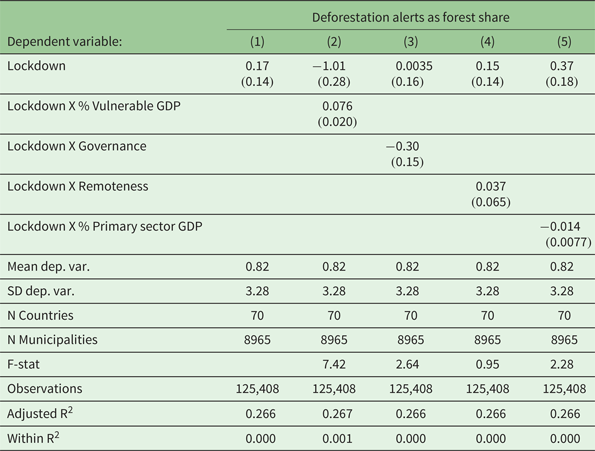
Notes: This table presents heterogeneous effects of estimating equation (2). Alerts as forest share are calculated as the number of pixels with deforestation alerts per 10,000 forest pixels. Column (2) assesses heterogeneous effects by the share of lockdown vulnerable GDP, measured as the share of wholesale, retail trade, restaurants, and hotel activities in the national economy. Column (3) explores heterogeneity by the level of government effectiveness using data provided by the Worldwide Governance Indicators of the World Bank. Column (4) explores heterogeneous effects of the remoteness of the municipality, measured as the standardized distance from the municipality to the capital. Column (5) presents heterogeneous effects by the share of the primary sector in the country's GDP. F-stat reports the F-statistic testing the joint significance of the lockdown and the interacted coefficient. Critical values F(2,$\infty$ ) at 5%: 3; 10%: 2.3. Clustered standard errors at the municipality and square bi-week level are in parentheses.
We restrict the analysis to Colombian municipalities in table 4. Colombia is an interesting case study, as it is the only large forest country where deforestation goes down following lockdowns (see appendix figure A4). For this country, we have municipality-level information on lockdown-vulnerable GDP and governance. We estimate only equation (3) because there is no variation in lockdown timing across Colombian municipalities. Column (1) shows a statistically significant reduction in deforestation with the 2020 COVID lockdown. In column (2), we interact the lockdown dummy with the percentage of lockdown-vulnerable GDP. The coefficient of the interaction is positive, which means that the reduction in deforestation was smaller in municipalities more affected economically by the lockdown. In column (3), we study heterogeneity by governance. Although the coefficient ($-0.27$ ) is not statistically significant, it is similar in magnitude to the one in table 3 ($-0.30$
 ) for all the countries. Column (4) then interacts the lockdown dummy with the municipality's relative remoteness. Similar to the global regression, we find that lockdown orders reduce deforestation more in municipalities close to the capital, and the effect is statistically different from zero. In column (5), we interact the lockdown indicator with the percentage of primary sector GDP. The coefficient is not statistically significant. But similar to the global results, it indicates lower deforestation for municipalities relying more on the primary sector. These Colombian results align with the global results that highlight the importance of alternative income sources and governance for protecting forests.
Table 4. Results for Colombia
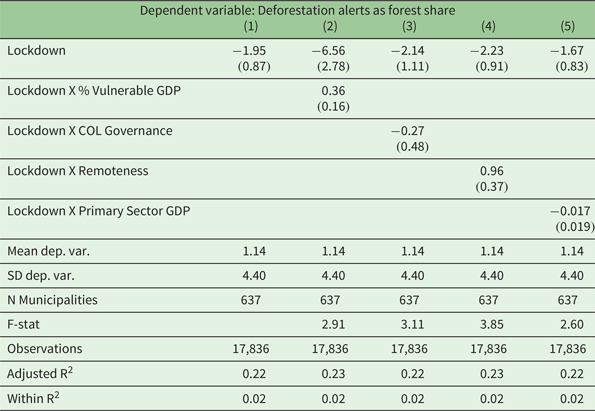
Notes: Alerts as forest share are calculated as the number of pixels with deforestation alerts per 10,000 forest pixels. Column (1) reports the coefficients obtained from the estimation of equation (3) for Colombian municipalities only. Column (2) explores the heterogeneous effect of lockdown-vulnerable GDP, measured as the share in the municipality economy of hotels, retail shops, and restaurants. Column (3) explores heterogeneity by the level of government effectiveness using the Municipal Performance Index provided by Colombia's National Planning Department. Column (4) explores heterogeneous effects of the remoteness of the municipality, measured as the standardized distance from the municipality to the capital. Column (5) shows heterogeneous effects by the percentage of the primary sector in the municipality in 2015 using Colombia's National Planning Department data. F-stat reports the F-statistic testing the joint significance of the lockdown and the interacted coefficient. Critical values F(2,83) at 5%: 3.11; 10%: 2.37. Clustered standard errors at the municipality and square bi-week level are in parentheses.
3.1 Robustness
Table A1 (appendix) reports the results of the robustness tests of the main results. First, we try different definitions of the lockdown start date in a country. Column (1) uses the date of the first COVID-19 case in each country, and column (2) employs a continuous measure of lockdown intensity. Column (3) uses the date of stay-at-home orders, and column (4) reports the results using the date when restrictions on internal movement were introduced. There were no statistically significant changes in deforestation when the lockdowns were imposed on these four cases. Column (5) explores heterogeneity by the week of the lockdown since people may have respected the lockdown order initially but stopped complying as they ran out of savings. However, the coefficients are similar and not statistically different from zero. Column (6) presents a Tobit model given that 30 per cent of the observations are zero; the coefficient is still not statistically different from zero. Column (7) explores the results using the number (rather than the share of forest area with alerts) as the dependent variable. The coefficient is also not statistically different from zero.
Table A2 (appendix) assesses how the noise in the deforestation alerts data affects the results. For comparison, columns (1) and (2) repeat the results in table 2, columns (5) and (6), respectively. Columns (3) and (4) present the same specifications but use data as of July 2020. As the data from the main specifications is from October 2020, fewer false positives were eliminated by July 2020. Columns (5) and (6) use 2019 data as of July 2019, so both years have the same lag in processing noise. In all cases, there were no statistically significant changes in deforestation rates when lockdowns were imposed.
Figure A3 in the appendix presents the Callaway and Sant'Anna (Reference Callaway and Sant'Anna2021) estimate of the lockdown effect on deforestation. The overall average treatment on the treated is $0.13 (0.16)$ with a confidence interval at the 95 per cent level of ($-0.18$
 ,0.45). We also cannot reject that deforestation did not change when countries were under lockdown. The two-way fixed effects estimated coefficients from table 2 are contained in this Callaway and Sant'Anna (Reference Callaway and Sant'Anna2021) interval and vice-versa. Reassuringly, the pattern of the dynamic effects of the lockdown by periods is similar to the one observed in figure 3B for the two-way fixed effects.
Table A4 in the appendix restricts table 2 to the municipalities for which we also have mobility data. The coefficient in all columns is not statistically different from zero. Appendix table A3 is analogous to table 2, but restricted to the countries that have ended the lockdown by the end of the study period. In most columns, there is no change in deforestation when the country is under lockdown. The coefficient in column (2) is positive and statistically significant, but in column (3) is negative and of similar magnitude. Finally, in figure A4 (appendix), we explore the effect of the lockdowns on deforestation in the countries with the largest forest area. The effect is not statistically different from zero for most of these countries.
3.2 Mechanism
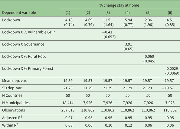
We explore how the lockdown orders affected the mobility behavior of citizens. This mechanism may explain the smaller reduction in deforestation in countries with high lockdown-vulnerable GDP and the higher reduction in deforestation in countries with an effective government. Table 5 presents regression results using the percentage change in mobility to workplaces as the dependent variable, as measured with Google's data. Column (1) shows that under lockdowns, there is an additional reduction of 6 percentage points in mobility in all municipalities of the countries for which we have data. Column (2) restricts the sample to the forest municipalities used in the main deforestation regression. Note that the effect of the lockdown orders is of similar magnitude, meaning that national lockdown orders have similar levels of compliance in forest municipalities. Columns (3)–(4) are the equivalent of columns (2)–(3) in table 3. We find that lockdown orders reduced commuting and that this reduction is smaller in countries with a high percentage of lockdown-vulnerable GDP. We also find larger mobility reductions in countries with good governance. These results align with deforestation results and suggest that deforestation is reduced when inhabitants comply with the lockdown orders. However, within a municipality, we cannot separate whether people's compliance in the urban center differs from those in rural areas. In Columns (5)–(6), the coefficients of the interactions are not statistically significant, so forest or rurality do not seem to be driving compliance. Table A4 in the appendix presents the main results (table 2) using the same observations as this table. Table A5 in the appendix shows results using the percentage of change in stay-at-home as the dependent variable.
Table 5. Effect of lockdown orders on mobility
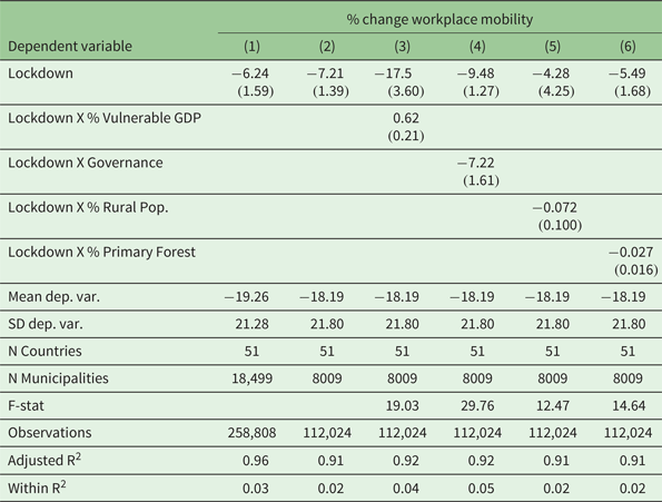
Notes: All columns include municipality and square bi-week fixed effects as estimating equation (2). The dependent variable is the percentage change in mobility to workplaces (Google LLC, 2020). Column (1) uses the sample of all municipalities, regardless of whether they have forests. Column (2) restricts the sample to municipalities with forests, i.e., municipalities in the deforestation regressions above. Column (3) assesses heterogeneous effects by the share of lockdown vulnerable GDP, measured as the share of wholesale, retail trade, restaurants, and hotel activities in the national economy. Column (4) explores heterogeneity by the level of government effectiveness using data provided by the Worldwide Governance Indicators of the World Bank. Column (5) shows the heterogeneous effect of the percentage of the rural population in the country, computed using the World Bank data. Column (6) presents the heterogeneous effect of the Primary Forest area. F-stat reports the F-statistic testing the joint significance of the lockdown and the interacted coefficient. Critical values F(2,$\infty$ ) at 5%: 3; 10%: 2.3. Clustered standard errors at the municipality and square bi-week level are in parentheses.
4. Conclusion
The COVID-19 lockdowns provide a case study of a policy that can potentially reduce deforestation. We use difference-in-differences strategies and satellite data to estimate what happened with deforestation during lockdowns. We find that, on average, deforestation was not affected by the lockdowns. This result contrasts with the observed reductions in cities’ pollution. There is, however, significant heterogeneity by the percentage of lockdown-vulnerable GDP. Countries and Colombian municipalities with a higher percentage of economic activity in sectors more affected by the lockdowns experienced smaller reductions and even increases in deforestation. We also find that deforestation decreased with lockdowns in countries and Colombian municipalities with more effective governments.
These results highlight that deforestation can be reduced when inhabitants have alternative income sources, and there is good governance. In the past, the main challenge associated with preventing deforestation was information. But real-time information on deforestation is no longer a barrier, thanks to advances in satellite data such as that used in this paper Moffette et al. (Reference Moffette, Alix-Garcia, Shea and Pickens2021). The challenge is to increase government capacity so that government officials can act on this information. And also provide alternative income sources to the population living close to forests. Future research could also examine why deforestation increased during lockdowns in Brazil or Mexico.
Supplementary material
The supplementary material for this article can be found at https://doi.org/10.1017/S1355770X23000153
Acknowledgements
Ivan de las Heras provided superb research assistance. We thank Mauricio Romero, Pedro Sant'Anna, Carolina Velez, and seminar participants at GoSee. The co-editor, associate editor and referees provided valuable comments that greatly improved this paper. We also thank Stanford University for allowing us to use Sherlock's computing resources.
Competing interest
The author declares none.
Appendix A
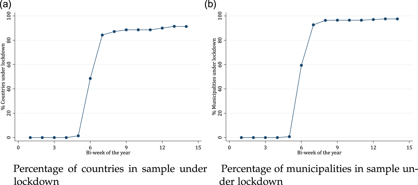
Figure A1. Sample under lockdown. (A) Percentage of countries in sample under lockdown, (B) Percentage of municipalities in sample under lockdown. Notes: Panel (A) presents the evolution of countries under lockdown in the main sample by bi-week of the year (2020). Panel (B) presents the percentage of municipalities under lockdown in the main sample.
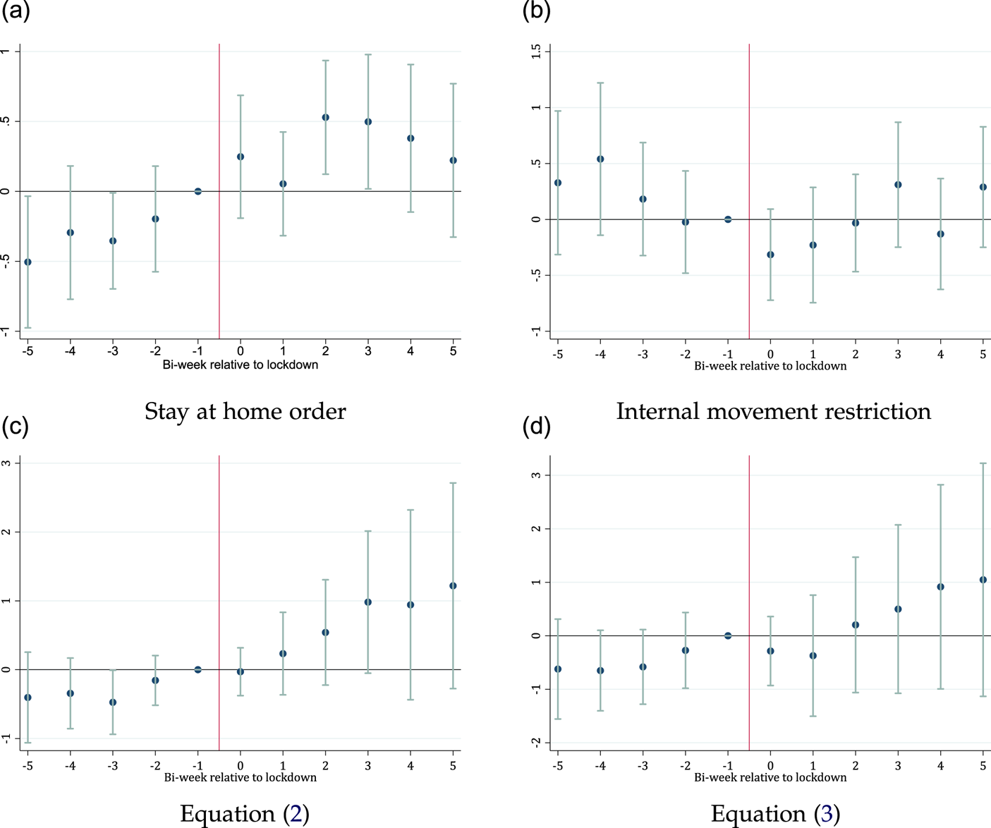
Figure A2. Dynamic specification. (A) Stay-at-home order, (B) Internal movement restriction, (C) Equation (2), (D) Equation (3), Notes: Panels (A) and (B) report the dynamic coefficients obtained from the estimation of equation (1). Panel (A) reports coefficients for the stay at home closure order. Panel (B) reports coefficients for the internal movement restriction. Panels (C) and (D) report the dynamic coefficients obtained from the estimation of equations (2) and (3), respectively together with 95% confidence intervals. The sample covers the window 5 bi-weeks before and 5 bi-weeks after the lockdown restriction.
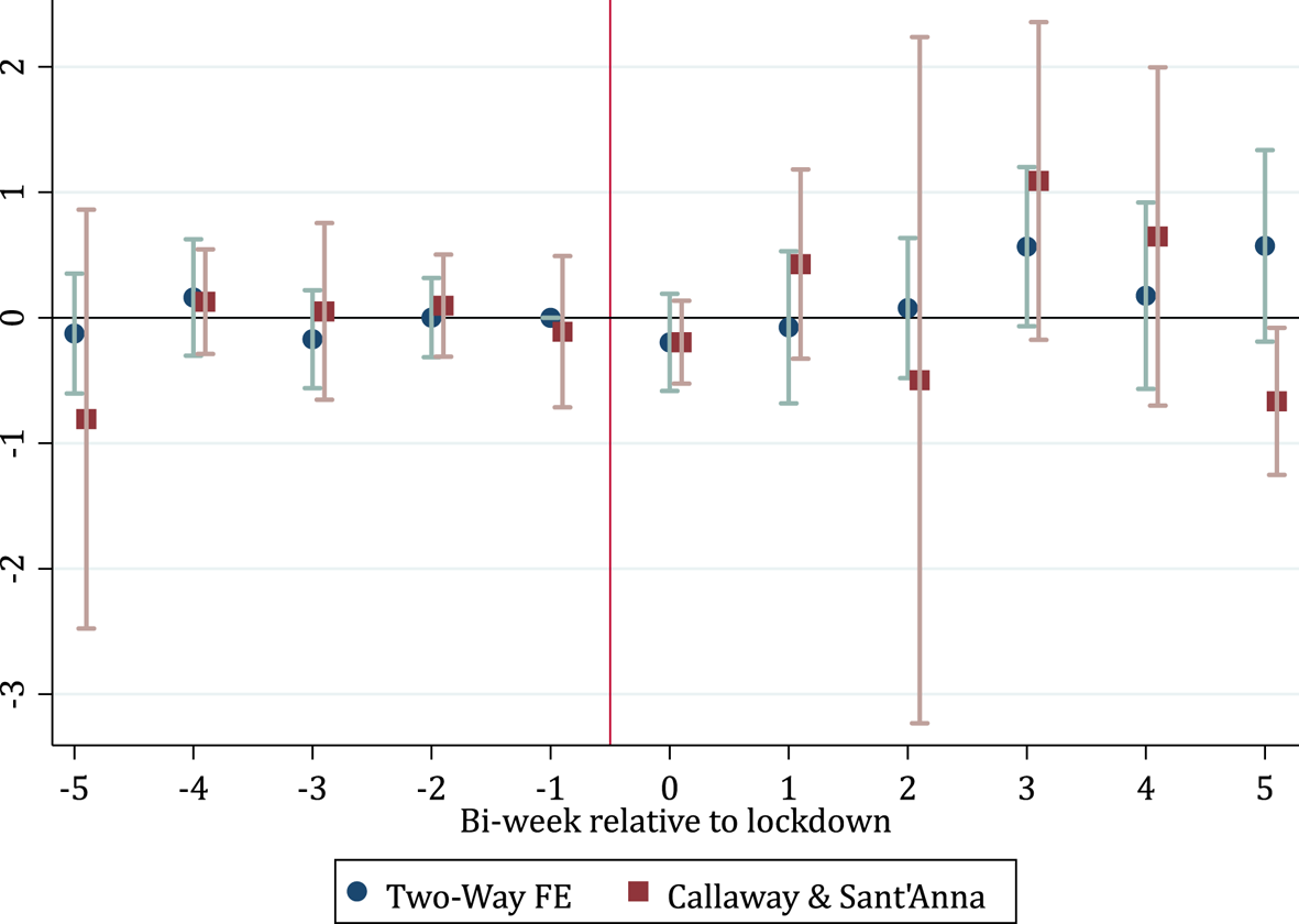
Figure A3. Callaway-Sant'Anna estimates. Notes: This figure presents the Callaway and Sant'Anna (Reference Callaway and Sant'Anna2021) decomposition of treatment effects by period. The y-axis presents the estimated effects relative to the lockdown timing (x-axis). The effects are slightly different from the one in table 2 because the Callaway and Sant'Anna (Reference Callaway and Sant'Anna2021) decomposition does not allow for non-monotonic treatment. Consequently, we exclude countries that end lockdown before bi-week 10.
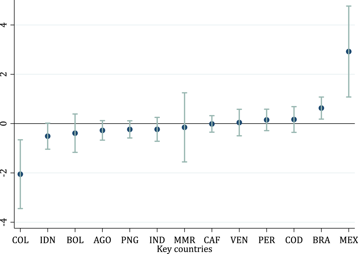
Figure A4. Heterogeneity by country. Notes: This figure reports the country lockdown coefficients obtained from the estimation of equation (1) together with 95% confidence intervals. The key countries are in order: Colombia (COL), Angola (AGO), Papua New Guinea (PNG), Indonesia (IDN), Bolivia (BOL), Central African Republic (CAF), Venezuela (VEN), Peru (PER), India (IND), the Democratic Republic of the Congo (COD), Brazil (BRA), Myanmar (MMR) and Mexico (MEX).
Table A1. Robustness.
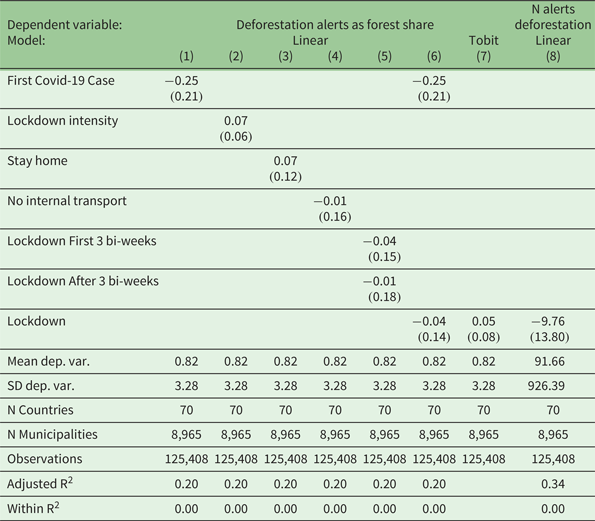
Table A2. Robustness to deforestation data cleaning.
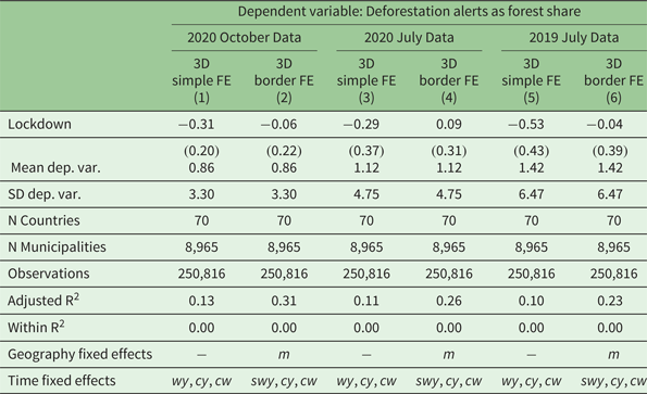
Table A3. Effect on countries whose lockdown order has ended.
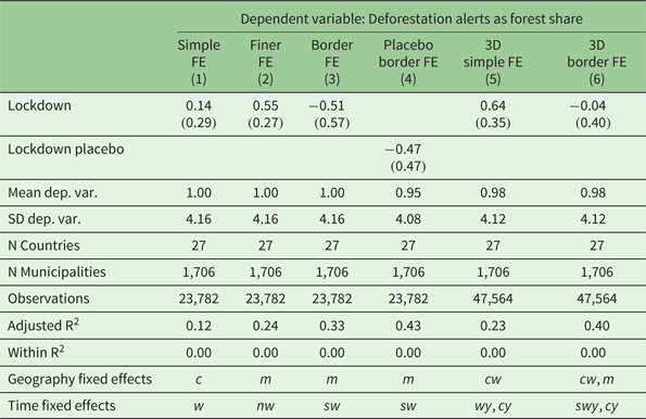
Table A4. Effect on countries with mobility data.
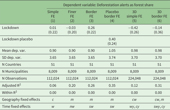
Table A5. Effect of lockdown orders on stay at home.