


1. Introduction
Rotor devices (e.g. propellers, wind and tidal turbines) that are initially designed to operate under uniform and axisymmetric flow are sometimes required to work in off-design conditions for manoeuvring (Felli & Falchi Reference Felli and Falchi2018; Huang, Qin & Pan Reference Huang, Qin and Pan2022) or optimal energy extraction (Li & Yang Reference Li and Yang2021; Borg et al. Reference Borg, Xiao, Allsop, Incecik and Peyrard2022). For instance, when a ship changes its direction, the lateral flow can strongly modify the propeller propulsive loads, thus affecting the ship dynamic response and inducing the thruster–hull interaction (Viviani et al. Reference Viviani, Bonvino, Mauro, Cerruti, Guadalupi and Menna2007; Dubbioso, Muscari & Di Mascio Reference Dubbioso, Muscari and Di Mascio2013, Reference Dubbioso, Muscari and Di Mascio2014; Di Mascio, Muscari & Dubbioso Reference Di Mascio, Muscari and Dubbioso2014; Zhang, Ma & Liu Reference Zhang, Ma and Liu2018; Qiu et al. Reference Qiu, Pan, Huang and Shi2020). Analogously, in a large wind farm, to avoid the unfavourable wake interaction between two wind turbines, an active yaw control strategy has been adopted to deflect the upstream turbine wakes away from the downwind turbines and to increase the total power production of the wind turbine array (Bastankhah & Porté-Agel Reference Bastankhah and Porté-Agel2016; Zong & Porté-Agel Reference Zong and Porté-Agel2020; Bossuyt et al. Reference Bossuyt, Scott, Ali and Cal2021; Li & Yang Reference Li and Yang2021). In this context, a deeper understanding of rotor wake dynamics and evolution mechanisms in an oblique flow is vital for optimizing rotor design and formulating control strategies.
Rotor wake vortex systems have been analysed for more than a century (Joukowsky Reference Joukowsky1912; Widnall Reference Widnall1972; Okulov & Sørensen Reference Okulov and Sørensen2007; Felli, Camussi & Di Felice Reference Felli, Camussi and Di Felice2011; Di Mascio et al. Reference Di Mascio, Muscari and Dubbioso2014). Conceptually, a rotor with N blades operating in a steady, axisymmetric flow consists of N tip vortices, N trailing edge vortices and N root vortices (or a hub vortex) (Okulov & Sørensen Reference Okulov and Sørensen2007; Micallef & Sant Reference Micallef and Sant2016). Each trailing edge vortex is generated by the spanwise gradient of the blade circulation ∂ $\varGamma$/∂r and is shed from the blade edge in a direction normal to the blade trailing edge. At the tip and root sections of each blade, the trailing edge vortex further rolls up into two counterrotating vortices, i.e. tip and root vortices, each with strength $\varGamma$ (Felli & Falchi Reference Felli and Falchi2018). Additionally, N root vortices coil around each other to form a hub vortex with strength −N $\varGamma$ (Okulov Reference Okulov2004; Zhang, Markfort & Porté-Agel Reference Zhang, Markfort and Porté-Agel2012; Ashton et al. Reference Allen and Auvity2016). When the rotor operates in a non-uniform or oblique flow, apart from the vortex structures mentioned above, the vortex systems also involve shed vortices, which are generated by the time-dependent blade circulation ∂ $\varGamma$/∂t and are shed in a direction parallel to the blade trailing edges (Di Mascio et al. Reference Di Mascio, Muscari and Dubbioso2014; Micallef & Sant Reference Micallef and Sant2016; Felli & Falchi Reference Felli and Falchi2018).
Tip vortices have attracted considerable attention due to their contribution to wake destabilization. The morphology of tip vortices and their instability are highly dependent on the blade geometry (e.g. blade number, blade skew and rake angles, as documented by Felli et al. Reference Felli, Camussi and Di Felice2011; Kumar & Mahesh Reference Kumar and Mahesh2017) and operative conditions (e.g. advance coefficient and inflow angle, see Di Mascio et al. Reference Di Mascio, Muscari and Dubbioso2014; Felli & Falchi Reference Felli and Falchi2018; Magionesi et al. Reference Magionesi, Dubbioso, Muscari and Di Mascio2018). Specifically, when a ring nozzle with a streamlined cross-section is fixed around a propeller, the tip vortices leaking from the gap between the blade tip and the nozzle inner sidewall undergo intense shear and vorticity redistribution (Wu, Ma & Zhou Reference Wu, Ma and Zhou2006), forming tip leakage vortices (Zhang & Jaiman Reference Zhang and Jaiman2019; Gong, Ding & Wang Reference Gong, Ding and Wang2021; Shi et al. Reference Shi, Wang, Zhao and Zhang2022). The tip vortices of the non-ducted propeller (NP) and the tip leakage vortices of the ducted propeller (DP) are referred to as helixes in this paper for brevity.
Under yawed conditions, asymmetric evolution, instability and breakdown of helixes were observed on the windward and leeward sides of the NP and DP (Dubbioso et al. Reference Dubbioso, Muscari and Di Mascio2013, Reference Dubbioso, Muscari and Di Mascio2014; Di Mascio et al. Reference Di Mascio, Muscari and Dubbioso2014; Felli & Falchi Reference Felli and Falchi2018; Huang et al. Reference Huang, Qin and Pan2022; Li et al. Reference Li, Huang, Pan, Dong and Li2022). For an NP operating in an oblique flow, a significant difference compared with the NP in an axisymmetric flow is the generation of the time-dependent shed vortices that induce the secondary vortex systems at the slipstream boundary via shear (Di Mascio et al. Reference Di Mascio, Muscari and Dubbioso2014; Felli & Falchi Reference Felli and Falchi2018). Moreover, the bending characteristics of the NP wake result in asynchronous helix ‘pairing’ on the leeward and windward sides (Felli & Falchi Reference Felli and Falchi2018). For yawed DPs, vortex shedding is generated at the leeward nozzle leading edge due to the yaw misalignment, and the interaction between the vortex shedding and the helixes accelerates wake destabilization in the leeward region (Huang et al. Reference Huang, Qin and Pan2022; Li et al. Reference Li, Huang, Pan, Dong and Li2022).
In large wind farms, an underlying mechanism that reduces power outputs and increases the fatigue loads of downwind turbines is far-wake meandering characterized by low-frequency and high-turbulence intensity (Viola et al. Reference Viola, Iungo, Camarri, Porté-Agel and Gallaire2015; Bastankhah & Porté-Agel Reference Bastankhah and Porté-Agel2017; Foti et al. Reference Foti, Yang, Campagnolo, Maniaci and Sotiropoulos2018a; Foti, Yang & Sotiropoulos Reference Foti, Yang and Sotiropoulos2018b; Mao & Sørensen Reference Mao and Sørensen2018; Yang & Sotiropoulos Reference Yang and Sotiropoulos2019; Li & Yang Reference Li and Yang2021). The misalignment of upstream wind turbine wakes with downstream turbines has attracted considerable attention as this strategy can effectively reduce the power losses caused by wake meandering (Bastankhah & Porté-Agel Reference Bastankhah and Porté-Agel2016; Micallef & Sant Reference Micallef and Sant2016; Foti et al. Reference Foti, Yang, Shen and Sotiropoulos2019; Zong & Porté-Agel Reference Zong and Porté-Agel2020; Bossuyt et al. Reference Bossuyt, Scott, Ali and Cal2021; Li & Yang Reference Li and Yang2021). Some literature has documented that wake meandering is related to the long-wave instability of the hub vortex (Felli et al. Reference Felli, Camussi and Di Felice2011; Iungo et al. Reference Iungo, Viola, Camarri, Porté-Agel and Gallaire2013; Viola et al. Reference Viola, Iungo, Camarri, Porté-Agel and Gallaire2014; Howard et al. Reference Howard, Singh, Sotiropoulos and Guala2015; Ashton et al. Reference Allen and Auvity2016; Foti et al. Reference Foti, Yang and Sotiropoulos2018b; Magionesi et al. Reference Magionesi, Dubbioso, Muscari and Di Mascio2018). However, a recent review by Yang & Sotiropoulos (Reference Yang and Sotiropoulos2019) concluded that hub vortex instability does not cause wake meandering but may energize large-scale motion, which is consistent with the findings of Kang, Yang & Sotiropoulos (Reference Kang, Yang and Sotiropoulos2014). Furthermore, a numerical investigation conducted by Foti et al. (Reference Foti, Yang, Campagnolo, Maniaci and Sotiropoulos2018a) reported that neither a nacelle model nor an unstable hub vortex is required for the existence of wake meandering. Mao & Sørensen (Reference Mao and Sørensen2018) modelled wake meandering without considering a hub vortex and noted that meandering is dominated by large-scale, low-frequency helical vortices experiencing a shear interaction with the free stream.
To explore the wake dynamic and destabilization mechanisms of a marine propeller, both experimental techniques, e.g. laser Doppler velocimetry (LDV) (Felli & Di Felice Reference Felli and Di Felice2005; Felli et al. Reference Felli, Camussi and Di Felice2011) and particle image velocimetry (PIV) (Di Felice et al. Reference Di Felice, Di Florio, Felli and Romano2004; Felli, Di Felice & Guj Reference Felli, Di Felice and Guj2006; Felli & Falchi Reference Felli and Falchi2018), and high-accuracy numerical models, such as large eddy simulation (LES) (Verma, Jang & Mahesh Reference Verma, Jang and Mahesh2012; Kumar & Mahesh Reference Kumar and Mahesh2017; Posa et al. Reference Posa, Broglia, Felli, Falchi and Balaras2019; Posa, Broglia & Balaras Reference Posa, Broglia and Balaras2020, Reference Posa, Broglia and Balaras2022; Posa & Broglia Reference Posa and Broglia2021; Wang et al. Reference Wang, Wu, Gong and Yang2021b; Wang, Liu & Wu Reference Wang, Liu and Wu2022), detached eddy simulation (DES) (Muscari, Di Mascio & Verzicco Reference Muscari, Di Mascio and Verzicco2013; Di Mascio et al. Reference Di Mascio, Muscari and Dubbioso2014; Muscari, Dubbioso & Di Mascio Reference Muscari, Dubbioso and Di Mascio2017; Wang et al. Reference Wang, Guo, Xu and Su2019; Gong et al. Reference Gong, Ding and Wang2021; Zhang et al. Reference Zhang, Ning, Li, Guo and Sun2021) and its variants, including detached DES (DDES) (Zhang & Jaiman Reference Zhang and Jaiman2019; Shi et al. Reference Shi, Wang, Zhao and Zhang2022) and improved DDES (IDDES) (Qin et al. Reference Qin, Huang, Pan, Han, Luo and Dong2021; Wang et al. Reference Wang, Wu, Gong and Yang2021a; Huang et al. Reference Huang, Qin and Pan2022; Li et al. Reference Li, Huang, Pan, Dong and Li2022), have been employed.
Furthermore, some postprocessing tools based on experimental and numerical results have been used to explore the evolution mechanisms of propeller wakes. For example, time-resolved velocity signals monitored by experimental LDV (Felli et al. Reference Felli, Camussi and Di Felice2011) or numerical probes (Shi et al. Reference Shi, Wang, Zhao and Zhang2022) are combined with time-frequency transform (or analysis) methods to explore the characteristic frequencies of flow phenomena and to investigate the energy transfer process in the propeller wake. The spectral analysis of individual spatial points can only qualitatively associate the flow signals with visible flow phenomena (Felli et al. Reference Felli, Camussi and Di Felice2011; Gong et al. Reference Gong, Ding and Wang2021; Wang et al. Reference Wang, Wu, Gong and Yang2021a; Shi et al. Reference Shi, Wang, Zhao and Zhang2022) but cannot visualize the flow phenomena with specific frequencies. An alternative way to address this problem is to decompose the whole flow field and visualize the spatial modes using machine learning-based, reduced-order models (ROMs, Rowley & Dawson Reference Rowley and Dawson2017; Taira et al. Reference Taira, Brunton, Dawson, Rowley, Colonius, McKeon, Schmidt, Gordeyev, Theofilis and Ukeiley2017; Brunton et al. Reference Brunton, Budišić, Kaiser and Kutz2022). Among various ROMs, proper orthogonal decomposition (POD, Lumley Reference Lumley1970; Sirovich Reference Sirovich1987) and dynamic mode decomposition (DMD, Rowley et al. Reference Rowley, Mezić, Bagheri, Schlatter and Henningson2009; Schmid Reference Schmid2010) are commonly applied data-driven methods.
The POD and/or DMD have been widely used in analysing rotor wake experimental PIV (Paik et al. Reference Paik, Kyung, Jung and Sang2010; Nemes et al. Reference Nemes, Sherry, Jacono, Blackburn and Sheridan2014; Felli, Falchi & Dubbioso Reference Felli, Falchi and Dubbioso2015; Kumar & Mahesh Reference Kumar and Mahesh2015; Bastankhah & Porté-Agel Reference Bastankhah and Porté-Agel2017) and numerical results (Sarmast et al. Reference Sarmast, Dadfar, Mikkelsen, Schlatter, Ivanell, Sørensen and Henningson2014; Iungo et al. Reference Iungo, Santoni-Ortiz, Abkar, Porté-Agel, Rotea and Leonardi2015; Debnath et al. Reference Debnath, Santoni, Leonardi and Iungo2017; Foti et al. Reference Foti, Yang, Campagnolo, Maniaci and Sotiropoulos2018a; Magionesi et al. Reference Magionesi, Dubbioso, Muscari and Di Mascio2018; Qatramez & Foti Reference Qatramez and Foti2021; Sun et al. Reference Sun, Tian, Zhu, Hua and Du2021; De Cillis et al. Reference De Cillis, Cherubini, Semeraro, Leonardi and De Palma2022a,Reference De Cillis, Cherubini, Semeraro, Leonardi and De Palmab; Shi et al. Reference Shi, Wang, Zhao and Zhang2022; Wang et al. Reference Wang, Liu and Wu2022). For a four-bladed propeller (blade frequency is four times the shaft frequency), Magionesi et al. (Reference Magionesi, Dubbioso, Muscari and Di Mascio2018), Shi et al. (Reference Shi, Wang, Zhao and Zhang2022) and Wang et al. (Reference Wang, Liu and Wu2022) identified that the passage of helixes and the pairing of adjacent helixes are characterized by blade frequency and half blade frequency, respectively. Moreover, low-frequency signals lower than or equal to the shaft frequency are associated with wake meandering (Magionesi et al. Reference Magionesi, Dubbioso, Muscari and Di Mascio2018), as further confirmed by Shi et al. (Reference Shi, Wang, Zhao and Zhang2022), Foti et al. (Reference Foti, Yang, Campagnolo, Maniaci and Sotiropoulos2018a) and Bastankhah & Porté-Agel (Reference Bastankhah and Porté-Agel2017) using reduced-order reconstruction. The modal analysis also enables the identification of other underlying destabilization mechanisms that are not easily detected in the spatiotemporally coupled flow field. For instance, based on the vorticity magnitude in the NP and DP wakes obtained by the DDES model, Shi et al. (Reference Shi, Wang, Zhao and Zhang2022) found that the helixes interact with trailing edge vortices at the blade frequency and its multiples, where the blade frequency mode dominates this interaction mechanism. Furthermore, during the vortex interaction at the blade frequency, helixes undergo short-wave instability, and numerous secondary vortices are formed between adjacent helixes. Sarmast et al. (Reference Sarmast, Dadfar, Mikkelsen, Schlatter, Ivanell, Sørensen and Henningson2014) locally analysed the velocity in the wind turbine wake achieved by LES and focused on the onset mechanism of helix instability. The authors discovered that an out-of-phase displacement of successive helixes characterizes the most unstable modes, and these modes cause the pairing of adjacent helixes, which is consistent with the findings of Sun et al. (Reference Sun, Tian, Zhu, Hua and Du2021).
Modal decomposition techniques have been widely employed in analysing the rotor wake in axisymmetric configurations. However, minimal attention has been given to the feasibility of the methods in oblique inflow conditions where several distinct but neighbouring spectral peaks may coexist in one successive helix as it travels downstream (Di Mascio et al. Reference Di Mascio, Muscari and Dubbioso2014). Another subject worth investigating is the effect of a nozzle on the propeller wake deflection and helix vorticity intensity in an oblique flow. The majority of studies compared only the wake dynamics of a single NP or DP operating at slight inflow angles (≤30°) (Dubbioso et al. Reference Dubbioso, Muscari and Di Mascio2013; Di Mascio et al. Reference Di Mascio, Muscari and Dubbioso2014; Felli & Falchi Reference Felli and Falchi2018; Huang et al. Reference Huang, Qin and Pan2022; Li et al. Reference Li, Huang, Pan, Dong and Li2022), but a comprehensive comparison of the wake characteristics of a propeller with and without a nozzle over a wide range of inflow angles is rare. In the present work, numerical research on the wake dynamics of an NP and DP with the same propeller geometry working at five inflow angles (α = 0°, 15°, 30°, 45° and 60°) is conducted to evaluate the effect of the nozzle on the wake deflection and to explore the differences in the evolution characteristics and destabilization mechanisms between NP wakes and DP wakes in an oblique flow. The propeller (S5810 R) and nozzle (1393 type 19A) geometries are chosen, as the DP is designed to eliminate the undesirable hub vortex (Cozijn, Hallmann & Koop Reference Cozijn, Hallmann and Koop2010; Cozijn & Hallmann Reference Cozijn and Hallmann2012; Maciel, Koop & Vaz Reference Maciel, Koop and Vaz2013; Koop et al. Reference Koop, Cozijn, Schrijvers and Vaz2017) and it gives us a chance to evaluate the far-wake meandering in yawed conditions without interference from a hub vortex. A moderate advance coefficient of J = 0.4 is chosen because this operating condition is full of rich destabilization mechanisms (Magionesi et al. Reference Magionesi, Dubbioso, Muscari and Di Mascio2018; Zhang & Jaiman Reference Zhang and Jaiman2019; Shi et al. Reference Shi, Wang, Zhao and Zhang2022).
In this paper, qualitative analysis of the wake destabilization, quantitative evaluation of the flow physics and spectrum-based modal identification methods are combined to gain a deeper insight into the rotor wake dynamics during realistic operational conditions. Figure 1 clarifies the structure of the paper and the links between two sections. The numerical setup is described in § 2. Comprehensive comparisons of destabilization mechanisms and wake deflection between NP wakes and DP wakes at different inflow angles are presented in § 3. Modal analysis of the wake vorticity based on POD and DMD is documented in § 4. The key conclusions are summarized in § 5.

Figure 1. Framework structure of the paper.
2. Numerical method
The DDES model developed by Spalart et al. (Reference Spalart, Deck, Shur, Squires, Strelets and Travin2006) is employed to simulate transient flow. The turbulence model is described in this section and grid sensitivity studies are presented separately in § A.1.
2.1. Governing equations
The wakes of the NP and DP are simulated by solving the three-dimensional (3-D) incompressible Navier‒Stokes equations. For an incompressible, single-phase Newtonian flow, the filtered mass and momentum equations are given by
 \begin{gather}\frac{{\partial {{\bar{u}}_i}}}{{\partial {x_i}}} = 0,\end{gather}
 \begin{gather}\frac{{\partial {{\bar{u}}_i}}}{{\partial t}} + \frac{{\partial {{\bar{u}}_i}{{\bar{u}}_j}}}{{\partial {x_j}}} ={-} \frac{1}{\rho }\frac{{\partial \bar{p}}}{{\partial {x_i}}} + \nu \frac{{{\partial ^2}{{\bar{u}}_i}}}{{\partial {x_i}\partial {x_j}}} - \frac{{\partial {D_{ij}}}}{{\partial {x_j}}},\end{gather}
 where  ${\bar{u}_i}$ is the fluid velocity, ρ is the fluid density, $\bar{p}$ is the fluid pressure, ν is the kinematic viscosity and $D_{ij} = \overline {{u_i}{u_j}} - {\bar{u}_i}{\bar{u}_j}$ is the hybrid turbulent stress, which is denoted in the DDES model as
 \begin{equation}D_{ij} = {\textstyle{2 \over 3}}k{\delta _{ij}} - 2{\nu _t}{\tilde{S}_{ij}},\end{equation}
where k is the turbulent kinetic energy,  ${\delta _{ij}}$ is the Kronecker delta, ${\nu _t}$ is the turbulent viscosity and ${\tilde{S}_{ij}}$ is the symmetric part of the velocity gradient.
As a hybrid Reynolds-averaged Navier‒Stokes (RANS)/LES model, the DDES model takes advantage of both the RANS model and the LES model. The RANS/LES model reduces the computational cost in the boundary layer region around the blades and nozzle compared with LES and has higher computational accuracy than the RANS model in simulating the wake. Compared with the original DES model (Shur et al. Reference Shur, Spalart, Strelets and Travin1999), the DDES model addresses ambiguous grid densities and more accurately simulates the near-wall flow and wake vortex structures.
The DDES model accurately predicts turbulence near the wall using a one-equation eddy viscosity model, namely, the Spalart–Allmaras (S-A) model (Spalart & Allmaras Reference Spalart and Allmaras1992). The ‘trip function’ with the ft 2 term in the original S-A model is excluded in the adopted S-A as it only slightly contributes to the fully turbulent computations (Rumsey Reference Rumsey2007). The turbulence models are presented in detail by Zhang & Jaiman (Reference Zhang and Jaiman2019) and Shi et al. (Reference Shi, Wang, Zhao and Zhang2022).
To simulate the rotation of the blades and hub of the rotor, the arbitrary mesh interface (AMI) approach is employed. This interface approach depends on the super mesh construction algorithm and enables a time-accurate simulation for rotating systems across disconnected and adjacent mesh domains. In the AMI approach, the rotating part covering the blades and hub is implemented inside the computational domain. The rotating and stationary domains are coupled across their interfaces using a conservative interpolation method via the local Galerkin projection proposed by Farrell & Maddison (Reference Farrell and Maddison2011). The governing equations are solved at cell centres in the finite volume domain. The equations for the continuity, momentum, turbulence and rigid body motion are independently solved for the rotor and stator domains.
During the calculations, we adopt a hybrid convection scheme (Travin et al. Reference Travin, Shur, Strelets and Spalart2002; Spalart et al. Reference Spalart, Shur, Strelets and Travin2012), which provides a blending between a low dissipative unbounded second-order convection scheme in the LES region and a robust unbounded second-order upwind scheme in the RANS region. The continuity, momentum and turbulence equations are solved by a hybrid solver, which combines the time-accurate pressure implicit with the splitting of operators (PISO) and the semi-implicit method for pressure-linked equations (SIMPLE) algorithms. Temporal discretization is achieved by the backwards-difference scheme with a second-order convergence. Linear equations resulting from the discretized equations are computed using Gauss‒Seidel and generalized geometric-algebraic multigrid (GAMG) solvers. All simulations are conducted using open-source computational fluid dynamics (CFD) software: open-source field operation and manipulation (OpenFOAM®v2112).
2.2. Numerical setup
The wake dynamics of a four-bladed, fixed-pitch, right-handed propeller (S5810 R) with and without a nozzle (1393 type 19A) operating in axisymmetric and oblique flows are compared in this study. The propeller and nozzle models are chosen because they are designed to eliminate the undesirable hub vortex (Cozijn et al. Reference Cozijn, Hallmann and Koop2010; Cozijn & Hallmann Reference Cozijn and Hallmann2012; Maciel et al. Reference Maciel, Koop and Vaz2013; Koop et al. Reference Koop, Cozijn, Schrijvers and Vaz2017) and allow us to investigate wake destabilization in the absence of hub vortex interference. Figures 2(a) and 2(b) show the geometries of the models. The parameters of the propeller and nozzle are listed in table 1. The rotor rotational speed, i.e. shaft frequency fshaft, is fixed at n = 17.65 rps (revolutions per second). The Reynolds number based on the rotational speed is  $R{e_n} = n{D^2}/\nu = 1.765 \times {10^5}$, where D = 0.1 m is the propeller diameter. The model parameters, rotational speed and Reynolds number are chosen to match previous experimental settings (Cozijn et al. Reference Cozijn, Hallmann and Koop2010; Cozijn & Hallmann Reference Cozijn and Hallmann2012) and numerical settings (Maciel et al. Reference Maciel, Koop and Vaz2013; Koop et al. Reference Koop, Cozijn, Schrijvers and Vaz2017).

Figure 2. (a,b) Geometries and (c) computational domain of the NP and DP cases. The displayed computational domain is out of proportion. (a) Front view, (b) side view and (c) side view of computational domain.
Table 1. Propeller (S5810 R) and nozzle (1393 type 19A) parameters (Maciel et al. Reference Maciel, Koop and Vaz2013).

The numerical simulations cover five flow oblique angles α = 0°, 15°, 30°, 45° and 60° for the NP and DP (figure 2c shows the definition of α), totalling ten cases, with a moderate advance coefficient  $J = {U_\infty }/nD = 0.4$, where ${U_\infty } = {(U_{x\infty }^2 + U_{y\infty }^2 + U_{z\infty }^2)^{0.5}}$ is the inflow velocity. Using the inflow velocity U∞ as the reference velocity does not apply to zero inflow velocity conditions, such as dynamic positioning systems or the moment the ship initiates in still water (Zhang & Jaiman Reference Zhang and Jaiman2019). Furthermore, the inflow velocity in the x direction ${U_{x\infty }} = {U_\infty }\cos \alpha$ (effective velocity aligned with the propeller axis) is unsuitable for the zero inflow velocity or high inflow angle (e.g. α = 90°) case. Therefore, the reference velocity for all cases in this paper is defined according to the blade tip velocity as ${U_{tip}} = n{\rm \pi}D \approx 5.54\;\textrm{m}\;{\textrm{s}^{ - 1}}$ for comparison purposes.
The computational domain is initially a round cylinder with a length of 26D and a diameter of 50D for zero inflow angle conditions. The computational domain is deformed according to the inflow angle (figure 2c) to anchor the wake to the core (grid encryption zone) of the computational domain and is sheared to ensure a consistent length of the domain in the x direction. The domain extends 3D upstream and 23D downstream of the NP or DP, and the blockage ratio  $\varepsilon = {A_d}/{A_c} = 0.0004$ (where Ad is the area of the propeller disk and Ac is the area of the domain's cross-section) is substantially less than the rule of thumb (ε < 0.1) suggested by Kumar & Mahesh (Reference Kumar and Mahesh2017) for a blockage effect-free solution.
The boundary conditions of the computational domain are specified as follows. The cylindrical boundary is set as a symmetry condition, and a no-slip boundary condition is specified at the solid surfaces of the propeller and nozzle. The velocity inlet (uniform velocity  ${U_\infty } = 0.706\;\textrm{m}\;{\textrm{s}^{ - 1}}$ with varying inclination angles) and pressure outlet boundary conditions are prescribed at the left inlet and right outlet of the computational domain.
The central part of the computational domain indicated in figure 2(c) is discretized by Pointwise® software into regular and smooth structured meshes. We strictly follow OpenFOAM and Pointwise mesh generation guidelines on skewness and minimum included angle to improve the mesh quality. Three different grid densities, i.e. coarse, medium and fine meshes, are used to conduct a grid sensitivity study in § A.1, and the fine mesh is chosen in this study (the mesh numbers are detailed in table 2). The surface mesh of the NP and DP is shown in figure 3. For each mesh configuration, the y + value at the solid surfaces of the NP and DP is below 5, with only a few exceptions (approximately 20 cells) located at blade tips.
Table 2. Fine meshes were used for each case.


Figure 3. Fine computational mesh near (a) the NP and (b,c) DP. (a) NP front view, (b) DP front view and (c) DP α = 60°, side view.
Using the steady flow solution calculated by the traditional multiple reference frame (MRF) method as the initial condition, the transient wake evolution is solved using the AMI dynamic mesh. The time step of the transient simulation is 1.575 × 10⁻⁵ s, which is the time for the propeller to rotate 0.1 degrees. The wake is fully developed and stabilized after 15 propeller revolutions. For each case, ten (16th–25th) revolutions of flow field data are recorded at an interval of 3 degrees of propeller rotation (Δt = 4.725 × 10⁻⁴ s), totalling 1200 snapshots.
3. Wake field analysis
This section discusses the differences in the wake evolution and destabilization mechanisms between the NP and DP in an oblique flow (α = 15°, 30°, 45° and 60°) based on the instantaneous vorticity magnitude  $\varOmega = {(\varOmega _x^2 + \varOmega _y^2 + \varOmega _z^2)^{0.5}}$. Subsequently, the deflection angles of various vortex systems are quantified to determine the effect of the nozzle on the propeller wake deflection.
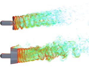
Figure 4 shows the volume rendering of instantaneous vorticity that displays semitransparent volumetric objects according to the vorticity value and figure 5 shows contours of instantaneous vorticity on the xy plane. According to the degree of instability, the outer portion of the NP and DP slipstream (slipstream is the high-speed stream past the rotor) is divided into three regions: the near-wake region, transition region and far-wake region. The near-wake region is close to the propeller disk, where helixes (tip vortices for the NP and tip leakage vortices for the DP) have well-defined helical morphology. The region where the helixes couple with other vortex systems and lose their original morphology is defined as the transition region. The far-wake region is where the helixes are broken down into small-scale, disordered turbulence. The three regions are separated by red and yellow dashed lines in figure 4.

Figure 4. Volume rendering of the normalized instantaneous vorticity magnitude  $\varOmega D/{U_{tip}}$ for the NP at (a) α = 0°, (c) 15°, (e) 30°, (g) 45° and (i) 60°, and the DP at (b) α = 0°, (d) 15°, (f) 30°, (h) 45° and (j) 60°. The three regions are separated by red and yellow dashed lines.

Figure 5. Contours of instantaneous vorticity magnitude  $\varOmega $ for the NP at (a) α = 0°, (c) 15°, (e) 30°, (g) 45° and (i) 60°, and the DP at (b) α = 0°, (d) 15°, (f) 30°, (h) 45° and (j) 60°. The vorticity is normalized by Utip/D.
The key findings in this section are the formation of a tube-shaped wake envelope (referred to as the vortex tube) and its subsequent rolling-up in the wake of the DP in an oblique inflow (figure 6). The generation mechanism of the vortex tube is ascribable to the similar vorticity intensity/magnitude between the helixes and the secondary vortices, which are discussed in detail below.

Figure 6. Schematic of the formation of a vortex tube and its rolling-up for the DP in an oblique flow.
3.1. Vortex interaction mechanisms
This subsection focuses mainly on the destabilization mechanisms of the helixes in the outer slipstream. For illustration purposes, ten cases are classified into two groups: Group 1 includes NP at α = 0°, 15°, 30°, 45° and 60°, and DP at α = 0°; Group 2 includes DP at α = 15°, 30°, 45° and 60°. The destabilization mechanisms in the outer slipstream of the two groups have significant differences.
Under axisymmetric conditions, tip vortices of the NP have a symmetric vorticity intensity and vortex core size/radius with respect to the propeller axis (figure 5a). When the propeller is confined in a nozzle (i.e. DP configuration), the nozzle exerts a shear on the tip vortices that leak from the gap between the blade tip and the nozzle, and the resulting tip leakage vortices undergo a vorticity redistribution on the nozzle inner sidewall (Gong et al. Reference Gong, Guo, Zhao, Wu and Song2018; Shi et al. Reference Shi, Wang, Zhao and Zhang2022), as shown in figure 5(b). Therefore, in an axisymmetric flow, the vorticity intensity of NP tip vortices is significantly higher than that of DP tip leakage vortices. For the NP in an oblique flow, time-dependent shed vortices and inhomogeneous blade circulation cause an asymmetric vortex core size of helixes, and the vortex core size is larger in the windward region than in the leeward region (figure 5c,e,g,i).
In the near-wake region of Group 1, the interaction between the trailing edge vortices and the helixes destabilizes the outer slipstream. As documented by Shi et al. (Reference Shi, Wang, Zhao and Zhang2022), the convection velocity of the trailing edge vortices is faster than that of the helixes; as a result, each trailing edge vortex disconnects from its corresponding helix and moves towards the downstream, previously shed helixes.
The torsion exerted on the helixes by the trailing edge vortices plays a crucial role in the short-wave instability of helixes, as highlighted by Ricca (Reference Ricca1994), Ahmed, Croaker & Doolan (Reference Ahmed, Croaker and Doolan2020), Gong et al. (Reference Gong, Ding and Wang2021) and Shi et al. (Reference Shi, Wang, Zhao and Zhang2022). During the interaction between the trailing edge vortices and the helixes, the vortex filaments in the helixes are ripped out by the trailing edge vortices, and consequently, the helixes undergo short-wave instability (areas enclosed by ellipses in figure 4a,b,c,e,g,i). Simultaneously, the trailing edge vortices shift the vortex filaments from the upstream helixes to the downstream helixes, forming secondary vortices between adjacent helixes (areas enclosed by circles in figure 5a,b,c,e,g,i).
The secondary vortices enhance the mutual inductance between adjacent helixes, and consequently, two adjacent helixes begin to pair/merge (rectangular boxes in figures 4a,b,c,e,g,i and 5a,b,c,e,g,i). In the transition region of Group 1, the dominant wake destabilization mechanism in the outer slipstream is helix pairing (Felli et al. Reference Felli, Camussi and Di Felice2011), which subsequently produces merged helixes (marked by rectangular boxes with rounded corners in figures 4a,b,c,e,g,i and 5a,b,c,e,g,i). The merged helixes are extremely unstable, with strong secondary vortices between them.
The generation mechanisms of secondary vortices are different in the near-wake and transition regions of Group 1. In the near-wake region, the secondary vortices are essentially vortex filaments ripped out by the trailing edge vortices from the helixes. However, in the transition region, the trailing edge vortices are gradually broken down due to viscous dissipation, and the secondary vortices are dominated by the shear exerted by the free stream on the merged helixes, consistent with the findings of Di Mascio et al. (Reference Di Mascio, Muscari and Dubbioso2014).
In Group 2, vortex shedding is defined as the phenomenon of flow separation from the nozzle as a result of the yawed misalignment. In figure 5(d,f,h,j), the vortex shedding from the leeward nozzle leading edge is stronger than that from the windward nozzle leading (significant only for the DP at α = 60°, as shown in figure 5j) and trailing edges.
In an oblique flow, the helixes of DP have a vorticity intensity similar to the secondary vortices due to the shear and vorticity redistribution experienced by the helixes on the nozzle inner sidewall. In the near-wake region of Group 2, the coupling between the helixes and the secondary vortices forms a coherent tube-shaped wake envelope (i.e. a vortex tube that separates the undisturbed flow from the slipstream, as shown in figure 5d,f,h,j), that is, the vortex tube is formed by a helix frame covered by secondary vortices.
The formation mechanisms of the vortex tube are different in the windward and leeward regions of Group 2. Figure 6 illustrates the four mechanisms that contribute to the generation of secondary vortices in the windward region: (i) the interaction between the trailing edge vortices and the helixes; (ii) the disturbance of the time-dependent shed vortices on helix formation and vorticity redistribution; (iii) the interference of the vortex shedding from the windward nozzle leading edge on the helix formation and vorticity redistribution, which is significant only for the DP at α = 60° (figure 5j); (iv) the interaction between the vortex shedding from the windward nozzle trailing edge and the helixes. In the leeward region of Group 2, in addition to mechanisms (i) and (ii), another decisive trigger to form the vortex tube is (v) the strong interaction between the vortex shedding from the leeward nozzle leading edge and the helixes, as illustrated in figures 4(d,f,h,j) and 5(d,f,h,j).
Since the vortex tube has been formed in the near-wake region of Group 2 due to the strong interaction among helixes, shed vortices and vortex shedding, the helix pairing phenomenon is invisible in the transition region. Instead, the rolling-up of the vortex tube is a new destabilization mechanism in the transition region of Group 2, especially in the windward region, as marked by rectangular boxes with rounded corners in figures 4(d,f,h,j) and 5(d,f,h,j). The rolling-up of the vortex tube in the present study is similar to the generation mechanism of vortex rings at the nozzle exit (Allen & Auvity Reference Allen and Auvity2002; Le et al. Reference Le, Borazjani, Kang and Sotiropoulos2011; Steinfurth & Weiss Reference Steinfurth and Weiss2020). The difference between them is that the former is a secondary instability process because the vortex tube consists of helixes and secondary vortices, but the latter is a primary process. During the downstream convection, the vortex tube always rolls up outwards with respect to the inner slipstream, and the rolling-up direction of the vortex tube matches the helix rotation direction (figure 6). Additional analysis of vortex tube rolling-up is provided in § 4.3.2 using modal decomposition techniques.
The trailing edge vortices entirely break down when the wake evolves to the far-wake region. Without the brace of the trailing edge vortices between the inner slipstream and the outer slipstream, the wake is susceptible to wiggling under the shear from the free stream. As a result, in the far-wake region of Groups 1 and 2, the dominant destabilization mechanism in the outer slipstream is wake meandering characterized as large-scale, low-frequency and stochastic (Felli et al. Reference Felli, Camussi and Di Felice2011; Magionesi et al. Reference Magionesi, Dubbioso, Muscari and Di Mascio2018), as shown in figures 4 and 5.
Wake meandering is a common phenomenon in wind farms (Kang et al. Reference Kang, Yang and Sotiropoulos2014; Howard et al. Reference Howard, Singh, Sotiropoulos and Guala2015; Viola et al. Reference Viola, Iungo, Camarri, Porté-Agel and Gallaire2015; Bastankhah & Porté-Agel Reference Bastankhah and Porté-Agel2016, Reference Bastankhah and Porté-Agel2017; Foti et al. Reference Foti, Yang, Guala and Sotiropoulos2016; Foti et al. Reference Foti, Yang, Campagnolo, Maniaci and Sotiropoulos2018a,Reference Foti, Yang and Sotiropoulosb; Mao & Sørensen Reference Mao and Sørensen2018; Gupta & Wan Reference Gupta and Wan2019; Li & Yang Reference Li and Yang2021), but its generation mechanism is still not fully understood. For the wind turbine and propeller wake, some previous investigations hypothesized that global meandering is ascribed to hub vortex distortions (Felli et al. Reference Felli, Camussi and Di Felice2011; Iungo et al. Reference Iungo, Viola, Camarri, Porté-Agel and Gallaire2013; Viola et al. Reference Viola, Iungo, Camarri, Porté-Agel and Gallaire2014; Howard et al. Reference Howard, Singh, Sotiropoulos and Guala2015; Ashton et al. Reference Allen and Auvity2016). However, without modelling a hub vortex, Mao & Sørensen (Reference Mao and Sørensen2018) and Foti et al. (Reference Foti, Yang, Campagnolo, Maniaci and Sotiropoulos2018a) found that stochastic wake meandering is driven by shear from the free stream and is dominated by large-scale vortices with helical morphology. Unfortunately, it is difficult to identify the generation mechanism of wake meandering via traditional flow visualization methods. Instead, modal decomposition techniques are employed to investigate the wake meandering mechanism in depth in § 4.3.4.
In the internal portion of the slipstream, the hub vortex is observed near the hub of the NP in axisymmetric and oblique flow conditions, as shown in figure 5(a,c,e,g,i). The hub vortex is formed by the coalescence of root vortices shed from the blade roots and the shear layers detached from the hub under the propeller rotation (Felli & Falchi Reference Felli and Falchi2018). However, the NP hub vortex is weak in this study, and additionally, the centrifugal effect of the DP nozzle further breaks down the weak hub vortex into chaotic turbulence (figure 5b,d,f,h,j). The breakdown of the hub vortex gives us a chance to investigate the far-wake meandering phenomenon without interference from hub vortex distortions.
For both the NP and DP in an oblique flow, the vortices shed from the propeller stem are referred to as inflow vortices, consistent with the findings of Felli & Falchi (Reference Felli and Falchi2018). The inflow vortices are strong in the wake of the NP and DP when the inflow angle α ≥ 45° (figure 5g,h,i,j). For the NP, the inflow vortices are coupled with the hub vortex, making it challenging to identify the hub vortex. However, for the DP, the inflow vortices have minimal effects on the fully destabilized chaotic turbulence.
3.2. Quantitation analysis of the wake deflection angle
An oblique flow significantly deflects the alignment angle of various vortex systems in the wake of the NP and DP. The deflection angles of wake vortices are different in the windward and leeward regions, and the hub vortex in the NP wake centre also has a distinct deflection angle. The deflection angle of each vortex system is determined based on the phase-averaged vorticity on the xy plane shown in figure 7. In figure 8, the locations of well-defined and merged helixes in the windward and leeward regions of the NP and DP wakes are mapped on the xy plane, and a linear fit is used to evaluate the deflection angle of the outer slipstream based on the locations of these well-defined and merged helixes. Note that NP helix 0 and DP helixes 0 to 2 in figures 7 and 8 are not considered in the linear fit because they are newly formed and unstable.

Figure 7. Contours of phase-averaged vorticity magnitude  $\varOmega $ for the NP at (a) α = 0°, (c) 15°, (e) 30°, (g) 45° and (i) 60°, and the DP at (b) α = 0°, (d) 15°, (f) 30°, (h) 45° and (j) 60°. The vorticity is normalized by Utip/D. The well-defined helixes marked by blue numbers are mapped on the xy plane in figure 8. Here, βh, βw and βl denote the deflection angle of the hub vortex, windward outer slipstream and leeward outer slipstream, respectively, as reported in figure 9; γw and γl defined in figure 7(b) denote the hydrodynamic pitch angle of the windward trailing edge vortex and leeward trailing edge vortex, respectively, as reported in figure 10.

Figure 8. Locations of the well-defined helixes (unfilled markers) and merged helixes (filled markers) on the (a,b) windward side and (c,d) leeward side of the NP and DP at α = 0°, 15°, 30°, 45° and 60°. Linear fits are used to evaluate the deflection angle of the outer slipstream. (a) NP windward, (b) DP windward, (c) NP leeward and (d) DP leeward.
Figure 9 shows the variations in the deflection angles of the hub vortex βh, and the windward βw and leeward βl outer slipstream with inflow angle α. For both the NP and DP in an oblique flow, the deflection angle of the outer slipstream is greater on the windward side than on the leeward side, as shown in figure 9(a). On the windward side, the deflection angle of the NP outer slipstream is higher than that of the DP outer slipstream at the same inflow angle when α ≥ 30°. Similarly, on the leeward side, the deflection angle of the DP outer slipstream is almost zero, and the deflection angle of the NP outer slipstream is always higher than that of the DP outer slipstream at the same inflow angle. For the NP in an oblique flow, the deflection angle of the hub vortex is always higher than that of the leeward outer slipstream, which implies that the hub vortex tends to penetrate the leeward outer slipstream. The deflection angle of the hub vortex at NP α = 60° is not considered because the inflow vortices from the propeller stem severely disturb the inner slipstream (figure 7i).

Figure 9. Inflow angle versus the (a) deflection angle and (b) deviation angle of the hub vortex and outer slipstream on the windward and leeward sides of the NP and DP at α = 0°, 15°, 30°, 45° and 60°. (c) Inflow angle versus the deflection and deviation angles of the NP and DP wake centre.
The angle deviation between the inflow angle α and the deflection angle β is defined as the deviation angle, α−β, which is positively correlated with the resistance of the wake against the inclined inflow. The deviation angle in figure 9(b) implies that oblique flow has a minimal effect on the leeward outer slipstream of the DP. Conversely, the windward outer slipstream of the DP, the windward and leeward outer slipstream of the NP, and the hub vortex of the NP are susceptible to deflection in an oblique flow, but their resistance against the oblique flow enhances with increasing inflow angle.
According to figure 7, for the NP and DP in an oblique flow, the deflection angle of the outer slipstream is different on the windward and leeward sides, so the fitted lines on the two sides necessarily have an intersection point in the wake region. Here, the line between the intersection point and the origin (0, 0) is defined as the nominal wake centre (different from the hub vortex) to measure the deflection of the overall wake (main flow), and the deflection and deviation angles of the nominal wake centre are reported in figure 9(c). The deflection angle of the NP and DP main flow follows approximately a linear function with the inflow angle, and the nozzle can effectively weaken the wake deflection in an oblique flow. In general, the resistance of the wake against the oblique flow can be ascribed to the following four factors: (i) shelter effect of the nozzle against oblique inflow; (ii) acceleration delivered by the propeller rotation; (iii) fluid viscosity; (iv) brace of the trailing edge vortices between the inner slipstream and the outer slipstream, as mentioned by Felli & Falchi (Reference Felli and Falchi2018).
In figure 7, an oblique flow also affects the hydrodynamic pitch angle γ of the trailing edge vortices (figure 7b), and the pitch angle of the first three unbroken trailing edge vortices is measured in figure 10. In the windward (leeward) region, the pitch angle is expected to decrease (increase) with increasing inflow angle due to wake deflection. However, for both the NP and DP, the inflow vortices that are shed from the propeller stem severely disrupt the inner slipstream and alter the pitch angle of the trailing edge vortices, especially when α ≥ 45° (figure 7).

Figure 10. Inflow angle versus the hydrodynamic pitch angle of the (a) first, (b) second and (c) third trailing edge vortices on the windward and leeward sides of the NP and DP at α = 0°, 15°, 30°, 45° and 60°.
The interference of the inflow vortices on the pitch angle of the trailing edge vortices is insignificant only in the NP windward region, where the pitch angles of the first three trailing edge vortices monotonically decrease with increasing inflow angle, with maximum variations of 20, 25 and 32 degrees for the first, second and third trailing edge vortices, respectively. For the first three trailing edge vortices in the NP leeward region, their variations in pitch angle with inflow angle are within 10 degrees, which is relatively moderate compared to the variations in the NP windward region. For the DP, under the shelter of the nozzle, the pitch angles of the first three trailing edge vortices in both the windward region and leeward region are insensitive to the inflow angle.
The velocity magnitude  $U = {(U_x^2 + U_y^2 + U_z^2)^{0.5}}$ is a desirable quantity to illustrate the velocity characteristics of various vortex systems as it is independent of the inflow angle and can show the differences in the deflection angle and value of the wake velocity for various cases. Figure 11 shows the profiles of the time-averaged velocity U along the lines of x/D = 0.4, 0.7, 1, 1.5, 2, 2.5 and 3 on the xy plane to evaluate the effects of an oblique flow on the wake velocity of the NP and DP.

Figure 11. Profiles of time-averaged velocity magnitude U of the (a) NP and (b) DP at α = 0°, 15°, 30°, 45° and 60°. The profiles are located at x/D = 0.4, 0.7, 1, 1.5, 2, 2.5 and 3 on the xy plane. The velocity is normalized by Utip.
In the axisymmetric condition with α = 0°, the minimum velocity of the NP and DP wakes is always in the hub region of approximately y/D = 0. Within 1D downstream of the propeller disk (x/D < 1), the maximum velocity of the NP wake at α = 0° is approximately |y/D| = 0.4, and this radial position moves outward to approximately |y/D| = 0.45 when the nozzle is mounted around the propeller, i.e. DP α = 0°. In figure 7(a,b), the helixes are located at approximately |y/D| = 0.5 for both the NP and DP at α = 0°, and |y/D| = 0.4 for the NP or 0.45 for the DP corresponds to the ends of the trailing edge vortices. The difference in the velocity value between |y/D| = 0.5 and |y/D| = 0.4 or 0.45 explains the destabilization mechanism that each trailing edge vortex interacts with the downstream, previously shed helixes, as detailed in § 3.1. Further downstream (x/D ≥ 1), the maximum velocity of the NP wake progressively shrinks towards the internal portion of the wake, but that of the DP wake is always at |y/D| = 0.45, which implies that the presence of the nozzle can inhibit the slipstream contraction behaviour (Felli et al. Reference Felli, Camussi and Di Felice2011; Di Mascio et al. Reference Di Mascio, Muscari and Dubbioso2014). Moreover, the nozzle reduces the wake velocity. Using the line of x/D = 0.4 at α = 0° as an example, the minimum velocity in the hub region of the wake is U/Utip = 0.09 for the NP and U/Utip = 0.06 for the DP, and the maximum velocity is U/Utip = 0.39 for the NP and U/Utip = 0.34 for the DP.
When the inflow is inclined, the oblique flow deflects the wake and alters the radial position and value of the maximum velocity. In figure 12(a–d), the locations of the local maximum velocity on the windward and leeward sides of the NP and DP wakes from x/D = 0.3 to 3 are mapped on the xy plane with the profiles spaced at x/D = 0.1. The alteration of the local maximum velocity's radial positions during the downstream convection is illustrated by the deflection angle of the maximum velocity βUmax, which is obtained by linear curve fitting of the data in figure 12(a–d). The variation in the deflection angle βUmax with inflow angle α is reported in figure 12(e). The evolution of the minimum wake velocity is not discussed as the strong flow coupling in the hub region of the wake makes it difficult to define the minimum velocity in each profile.

Figure 12. Locations of the peaks of time-averaged velocity magnitude U on the (a,b) windward side and (c,d) leeward side of the NP and DP at α = 0°, 15°, 30°, 45° and 60°. A linear fit is applied to evaluate the deflection angle of the velocity peak. (e) Inflow angle versus the velocity peak deflection angle. (a) NP windward, (b) DP windward, (c) NP leeward, (d) DP leeward and (e) statistics.
For both the NP wake and DP wake, the deflection angle βUmax on the windward side is higher than that on the leeward side due to the direct interaction of the windward wake with the oblique flow. Moreover, compared with the deflection angle βUmax on the NP leeward side, the shelter effect of the nozzle significantly reduces the deflection angle βUmax on the DP leeward side, especially for α ≥ 30°.
For the value of the maximum velocity, an apparent difference between the NP at α = 15° and 30° and the NP at α = 45° and 60° is observed in figure 11. At x/D = 0.4 and 0.7, the maximum velocity values of the NP at α = 15° and 30° are approximately equivalent to that of the NP at α = 0° on both the windward side and leeward side. As the inclination angle is further increased, on the NP leeward side, the maximum velocity values at α = 45° and 60° approximate those at α = 0°, 15° and 30°. However, on the NP windward side, the maximum velocity values at α = 45° and 60° are significantly higher than those at α = 0°, 15° and 30°, and the difference in the maximum velocity values increases with increasing inflow angle (as shown in the x/D = 0.4 and 0.7 profiles in figure 11a).
A contrary trend is observed in the DP windward region at x/D = 0.4 and 0.7 (figure 11b). The maximum velocity values in the DP windward region decrease with increasing inflow angle due to the obstruction of the inflow by the nozzle. However, the maximum velocity values in the DP leeward region are still insensitive to the inflow angle, following the same trend as those in the NP leeward region.
4. Modal analysis
In this section, two modal decomposition techniques, proper orthogonal decomposition (POD, Lumley Reference Lumley1970; Sirovich Reference Sirovich1987) and dynamic mode decomposition (DMD, Rowley et al. Reference Rowley, Mezić, Bagheri, Schlatter and Henningson2009; Schmid Reference Schmid2010), are employed to analyse space-frequency information in the NP and DP wakes. Detailed theories of POD and DMD are provided in § A.2.
4.1. Dataset
Both POD and DMD are performed based on the snapshot matrix X, which includes the variable being analysed and the spatial n and temporal m dimensions.
4.1.1. Analysis variable
Our previous study demonstrated that the modes obtained based on the vorticity magnitude can resolve various wake vortex structures and their instability (Shi et al. Reference Shi, Wang, Zhao and Zhang2022). Thus, the vorticity is still chosen for modal analysis in the present work.
According to Chen, Tu & Rowley (Reference Chen, Tu and Rowley2012) and Tu et al. (Reference Tu, Rowley, Luchtenburg, Brunton and Kutz2014), subtracting the mean data from the dataset allows the POD eigenvalues (square of singular values  $\sigma _i^2$) to be interpreted as the variance in fluctuations, but it might reduce the DMD to the temporal discrete Fourier transform (DFT). The removal of the mean data would distribute all DMD modes at a uniform frequency interval and disturb the frequencies of non-periodic modes. Therefore, the mean vorticity is retained in the datasets for DMD but is subtracted from the datasets for POD.
4.1.2. Spatial dimension of the snapshot matrix
The mesh number of the computational domain determines the spatial dimension n of snapshots. To reduce the calculation costs, a cylindrical computational subdomain with 7D in length (x/D = −1 to 6) and 4D in diameter (|z/D| = 0 to 2, and |y/D| = 0 to 2 for axisymmetric conditions and y/D = −1 to 3 for oblique flow conditions) is chosen to ensure that the core flows are contained in the subdomain. Moreover, the dynamic domain contained in the subdomain is not considered as the time delay in the data transmission between the dynamic domain and stationary domain might affect the modal decomposition (Magionesi et al. Reference Magionesi, Dubbioso, Muscari and Di Mascio2018; Shi et al. Reference Shi, Wang, Zhao and Zhang2022; Wang et al. Reference Wang, Liu and Wu2022). The mesh numbers of the subdomain for the ten cases are listed in table 3.
Table 3. Mesh number of the computational subdomain for the ten cases.

4.1.3. Temporal dimension of the snapshot matrix
The snapshot number m in the dataset depends on the snapshot sampling time interval and sampling size. The sampling time interval must be sufficiently small to resolve the high-frequency flows and the sampling size must be sufficiently long to record the low-frequency phenomena. Based on the modal convergence analysis in § A.3, datasets with a sampling time interval of  $\Delta {t_s} = \Delta t = 4.725 \times {10^{ - 4}}\;\textrm{s}$ and a sampling size of nine propeller revolutions are chosen for modal analysis, with 1080 POD and DMD modes in each case.
4.2. Modal statistics
To select a subset of POD and DMD modes that dominates the wake destabilizations, a sparse selection method is necessary to identify the critical modes. This section will identify the dominant modes according to the POD and DMD spectra.
4.2.1. Energy and spectra of POD modes
Figure 13 shows the relative and cumulative energy of POD modes based on (A3). The relative energy of each mode reflects the spatial information the mode contains, while the convergence rate of the cumulative energy curve is related to flow destabilization. The convergence rate of the energy content of a severely destabilized wake is generally slow because the disordered small-scale turbulence occupies a considerable proportion of the energy content (Magionesi et al. Reference Magionesi, Dubbioso, Muscari and Di Mascio2018; Shi et al. Reference Shi, Wang, Zhao and Zhang2022). For the NP and DP wakes at α = 0°, 15°, 30°, 45° and 60°, the first 404, 420, 477, 608, 657 modes and 189, 206, 207, 249, 423 modes, respectively, reach 99 % of the total modal energy, which indicates that the convergence rate of the cumulative energy decreases with increasing inflow angle (figure 13c,d), but the nozzle of DP can accelerate the energy convergence.

Figure 13. (a,b) Relative and (c,d) cumulative energy of POD modes for the NP and DP cases. (a) NP relative energy, (b) DP relative energy, (c) NP cumulative energy and (d) DP cumulative energy.
Figure 14 shows the normalized PSD (i.e. POD spectra) obtained by performing the fast Fourier transform on the time coefficient of each POD mode (A2), with the black pixels representing the location of spectral peaks. Only the spectra of the NP and DP at α = 0°, 45° and 60° are shown here. The spectra of the remaining NP and DP cases are similar to the results at α = 0°. The non-dimensional frequency is defined as  $\kappa = f/\,{f_{shaft}} = f/17.65$, where f is the modal frequency and fshaft is the shaft frequency. For the four-bladed rotor, the non-dimensional shaft frequency is denoted by κ = 1, the half blade frequency is κ = 2 and the blade frequency is κ = 4.

Figure 14. Spectral peak distribution of POD modes for the NP at (a) α = 0°, (c) 45° and (e) 60° and the DP at (b) α = 0°, (d) 45° and (f) 60°. The PSD is normalized by the spectral peak value of each mode.
For both the NP wake and DP wake, the spectral peaks of the POD modes are linear functions of the modal order. However, the modal order of a few modes dramatically drops away from the diagonal line and moves to the left; this drop is referred to as the ‘jumping-order’, as illustrated by the zoom-in view in figure 14. Shi et al. (Reference Shi, Wang, Zhao and Zhang2022) reported that the jumping order is a characteristic behaviour of dominant POD modes. For the NP wake, the jumping-order modes are characterized by spectral peaks at κ = [2: 2: 60] (i.e. κ = 2, 4, 6, …, 60). For the DP wake, the jumping-order behaviour of the modes with spectral peaks at κ = [2: 4: 58] (i.e. κ = 2, 6, 10, …, 58) is not significant compared with that of NP, and the jumping-order behaviour of these modes gradually weakens with increasing inflow angle.
4.2.2. Eigenvalues and spectra of DMD modes
The importance of each DMD mode is quantified by the dynamic factor  ${d_i} = |{s_i}|\times |{\lambda _i}{|^m}$ proposed by Statnikov, Meinke & Schröder (Reference Statnikov, Meinke and Schröder2017), where superscript ‘m’ is the snapshot number, and si and λi are the amplitude and eigenvalue, respectively, of the DMD mode, as shown in (A10). In addition to amplitude |si|, a decay term $|{\lambda _i}{|^m}$ in the dynamic factor can identify transient or spurious modes with high amplitudes but high decay rates. The dynamic factor of each mode is normalized by the maximum dynamic factor in each case. Similar to the sparsity-promoting (SP) method (Jovanović, Schmid & Nichols Reference Jovanović, Schmid and Nichols2014), the dynamic factor method was demonstrated to be effective for identifying the dominant modes in the rotor wake (Magionesi et al. Reference Magionesi, Dubbioso, Muscari and Di Mascio2018; Shi et al. Reference Shi, Wang, Zhao and Zhang2022).
According to the DMD spectra in figure 15, the DMD modes can be classified into four clusters (the modal clusters are independent of the group classification of destabilization mechanisms in § 3.1): (i) κ = [4: 4: 60]; (ii) κ = [2: 4: 58]; (iii) κ = [1: 2: 59]; and (iv) among the leading 25 modes with the highest dynamic factors, with the exception of the modes in the first three clusters, the remaining modes are classified as Cluster 4. Magionesi et al. (Reference Magionesi, Dubbioso, Muscari and Di Mascio2018) and Shi et al. (Reference Shi, Wang, Zhao and Zhang2022) classified similar modal clusters for the propeller wake based on SP-DMD and the reduced-order reconstruction method, respectively. Analogously, the cluster classification of DMD modes is also effective for POD modes according to the modal jumping-order behaviour in figure 14.

Figure 15. Spectral distribution of DMD modes for the (a) NP cases and (b) DP cases. The DMD spectra are normalized by the maximum dynamic factor in each case.
In Clusters 1–3, the dynamic factor (importance) in each cluster decreases with increasing modal frequency. Cluster 1 is important for both the NP wake and DP wake, and its importance is not influenced by the inflow angle α. The importance of Cluster 2 is higher in the NP wake than in the DP wake, and the importance of Cluster 2 in the NP wake decreases with increasing α. Cluster 3 is important only for the NP at α = 0°. The number of modes in Cluster 4 reflects the degree of wake instability. With the aggravation of wake instability, some high-frequency modes in Clusters 1–3 become insignificant and the number of modes in Cluster 4 increases.
Figure 16 shows the eigenvalue distribution of DMD modes for the NP and DP at α = 60°. Assuming that a DMD mode has a complex eigenvalue of  ${\lambda _i} = a + \textrm{i}b$, the modal frequency and growth/decay rate are denoted as
 \begin{align}{g_i} + \textrm{i}2{\rm \pi}{f_i} = \ln ({\lambda _i})/\Delta {t_s} = \ln (a + \textrm{i}b)/\Delta {t_s} = \ln (a2 + {b^2})/(2\Delta {t_s}) + \textrm{i}\,{\tan ^{ - 1}}(b/a)/\Delta {t_s},\end{align}
Figure 16. Eigenvalue distribution of DMD modes for the (a) NP at α = 60° and the (b) DP at α = 60°. The eigenvalues of low-frequency modes with κ ≤ 4 are shown enlarged on the right.
as shown in (A6) and (A7). Consequently, pairs of eigenvalues with the same frequency are symmetric with respect to the real axis, and the modal frequency increases with increasing argument. The growth/decay rate of modes is represented by the absolute value of their eigenvalues. Even for the severely destabilized wakes of the NP and DP at α = 60°, the eigenvalues are tightly clustered along the unit circle except for a few outliers (i.e. transient or spurious modes). Therefore, most modes have nearly zero growth/decay rates, indicating that the modes converge (Aaron, Schmidt & Colonius Reference Aaron, Schmidt and Colonius2018).
4.3. Modal results
Based on the modal classification in § 4.2.2, the spatial and temporal characteristics of the dominant modes in the four clusters are discussed in this section. Since the mean flow is not subtracted from the datasets for DMD, DMD identifies the mean flow modes as the κ = 0 modes in figure 16. The mean flow modes present only a mean vorticity distribution but have no contribution to the turbulence effects in the wake. In addition, according to previous reduced-order reconstruction results (Shi et al. Reference Shi, Wang, Zhao and Zhang2022), the spatial scale of modes decreases with increasing modal frequency. The low-frequency modes in each cluster play a dominant role in reproducing large-scale flow structures, while the contribution of high-frequency modes to the wake dynamics is small. Therefore, both zero-frequency and high-frequency modes are not discussed in this section.
4.3.1. κ = 4
Figures 17 and 18 demonstrate the first POD mode and the κ = 4 DMD modes, respectively. The iso-surface value and the legend of contours are not detailed in the modal visualization as the POD and DMD modes represent only the flow morphologies in space, and the iso-surface values and the minimum and maximum values of the contours have no physical relevance (Hamilton, Tutkun & Cal Reference Hamilton, Tutkun and Cal2015; Noack et al. Reference Noack, Stankiewicz, Morzyński and Schmid2016; Magionesi et al. Reference Magionesi, Dubbioso, Muscari and Di Mascio2018). The combination of the spatial modes with the time coefficients ((A2) for POD and (A9) for DMD) is applied to reconstruct the wake field (Shi et al. Reference Shi, Wang, Zhao and Zhang2022).

Figure 17. Iso-surfaces (left) and contours (right) of the first POD modes for the NP at (a) α = 0°, (c) 15°, (e) 30°, (g) 45° and (i) 60°, and the DP at (b) α = 0°, (d) 15°, (f) 30°, (h) 45° and (j) 60°.

Figure 18. Iso-surfaces (left) and contours (right) of the κ = 4 DMD modes for the NP at (a) α = 0°, (b) 15°, (c) 30°, (d) 45° and (e) 60°.

Figure 18. (Continued). Iso-surfaces (left) and contours (right) of the κ = 4 DMD modes for the DP at (f) α = 0°, (g) 15°, (h) 30°, (i) 45° and (j) 60°.
The κ = 4 DMD modes in figure 18 are correlated to the interaction between the trailing edge vortices and the helixes. Compared with the spatiotemporally coupled vorticity field in figure 5, the modal decomposition methods better identify the individual helixes in the outer slipstream, especially for the DP wakes in an oblique inflow where the helixes are coupled with the secondary vortices into a vortex tube. Furthermore, the occurrence of helix short-wave instability at the frequency of κ = 4 indicates that the short-wave instability is caused by the torsion exerted on the helixes by the trailing edge vortices during their interaction, as reported by Ricca (Reference Ricca1994), Ahmed et al. (Reference Ahmed, Croaker and Doolan2020), Gong et al. (Reference Gong, Ding and Wang2021) and Shi et al. (Reference Shi, Wang, Zhao and Zhang2022).
Another destabilization mechanism characterized by κ = 4 is the merging between the helixes and the ends of the trailing edge vortices, as marked by rectangular boxes in figure 18. Since the trailing edge vortices are susceptible to viscous dissipation, they gradually break down during downstream convection, and subsequently, the broken trailing edge vortices merge with the helixes under the induction of the helixes.
Moreover, in the windward region of the DP at α = 60°, the vortex shedding from the windward nozzle leading edge and the time-dependent shed vortices perturb the vorticity distribution on the nozzle inner sidewall (figures 5 and 6). The vorticity on the nozzle inner sidewall is involved in the formation of the helixes, while the unused vorticity is induced by the trailing edge vortices to form the strong trailing edge vortex ends near the helixes. However, the strong trailing edge vortex ends are easily separated from the trailing edge vortices and form additional vortex structures that are independent of the helixes and the trailing edge vortex main bodies, as shown in figure 18(j). Note that the trailing edge vortex ends are not separated from the trailing edge vortices in the spatiotemporally coupled vorticity field in figure 5(j) because the disconnected part of the trailing edge vortices are characterized by other frequencies and are invisible in the κ = 4 mode.
In figures 17 and 18, the spatial morphologies of the κ = 4 DMD modes are similar to those of the first POD modes. DMD modes have a single-frequency characteristic, but the first POD modes are characterized by multiple frequencies, with a dominant spectral peak at κ = 4, a second lower peak at κ = 8, a third lower peak at κ = 12, etc. (figure 17). To investigate the temporal characteristics of the POD and DMD modes, figure 19 illustrates the time coefficients of the first and second POD modes and the real and imaginary parts of the κ = 4 DMD modes, and the Lissajous figure is further applied to depict the phase portraits and to evaluate the phase difference between the time coefficients of the mode pairs, as shown in figure 20. The circular trajectories of the real and imaginary parts of the κ = 4 DMD modes imply that their time coefficients follow a sinusoidal function but with a 90-degree phase shift. However, for the first and second POD modes, their multifrequency characteristics (figure 17) and amplitude fluctuations (figure 19) result in irregular circular trajectories in figure 20.

Figure 19. Time coefficients of the first and second POD modes and the real and imaginary parts of the κ = 4 DMD modes for the NP at (a) α = 45° and (c) 60°, and the DP at (b) α = 45° and (d) 60°.

Figure 20. Phase portraits of the first and second POD modes and the real and imaginary (imag.) parts of the κ = 4 DMD modes for the NP at (a) α = 45° and (c) 60°, and the DP at (b) α = 45° and (d) 60°.

Figure 21. Iso-surfaces (left) and contours (right) of the κ = 2 DMD modes for the NP at (a) α = 0°, (b) 15°, (c) 30°, (d) 45° and (e) 60°.
For periodic flow phenomena, the real and imaginary parts of a complex DMD mode ϕi can be approximately represented by the pair of same-frequency POD modes  ${\boldsymbol{\psi }_j} + \textrm{i}{\boldsymbol{\psi }_{j + 1}}$ (Schmid, Violato & Scarano Reference Schmid, Violato and Scarano2012). Even if the POD mode pair has multiple spectral peaks, the two POD modes have similar spatial morphologies to the corresponding complex DMD mode if the POD modes have the same dominant spectral peak as the single-frequency DMD mode (Shi et al. Reference Shi, Wang, Zhao and Zhang2022). The frequency matching holds for the κ = 4 DMD modes and the first and second POD modes in the present work.
For both POD mode and DMD mode, their spatial scale decreases with increasing frequency. According to Magionesi et al. (Reference Magionesi, Dubbioso, Muscari and Di Mascio2018) and Shi et al. (Reference Shi, Wang, Zhao and Zhang2022), the κ = 8 DMD mode (or the POD mode with a dominant spectral peak at κ = 8) has the same spatial features as the κ = 4 DMD mode (or the POD mode with a dominant spectral peak at κ = 4), but the spatial scale of the former high-frequency mode is half that of the latter low-frequency mode. Furthermore, based on the DMD reconstruction, Shi et al. (Reference Shi, Wang, Zhao and Zhang2022) reported that the large-scale mode characterized by κ = 4 is dominant in the modal cluster κ = [4: 4: 60], and the remaining κ = [8: 4: 60] modes mainly add small-scale flow features. Therefore, high-frequency modes with κ > 4 are not the focus of this work and are not shown here for the sake of conciseness.
Since the spatial morphologies of DMD modes are similar to those of the corresponding POD modes and the single-frequency characteristic of DMD modes is convenient for seeking the physical relevance of the modes, the modal analysis in the remaining discussion is mainly based on the DMD modes.
4.3.2. κ = 2
The κ = 2 DMD modes shown in figure 21 are mainly associated with the merging of adjacent helixes, especially for the NP at α = 0°, 15°, 30°, 45°, 60° and the DP at α = 0° (i.e. Group 1; details in § 3.1), where the helix pairing phenomenon is visible in the outer slipstream in figures 4 and 5. However, for the DP at α = 15°, 30°, 45°, 60° (i.e. Group 2), a vortex tube is formed in the outer slipstream, followed by the rolling-up of the vortex tube in the windward region (figures 4 and 5). Therefore, the pairing between adjacent helixes is invisible in the spatiotemporally coupled flow field of Group 2.

Figure 21. (Continued). Iso-surfaces (left) and contours (right) of the κ = 2 DMD modes for the DP at (f) α = 0°, (g) 15°, (h) 30°, (i) 45° and (j) 60°.
In general, if the rolled-up vortex tube does not contain any helixes, its generation should be a stochastic process and its characteristic frequency should not be κ = 2. However, the helix pairing characterized by κ = 2 occurs in the windward region of Group 2 (figure 21g,h,i,j), implying that the rolled-up vortex tube contains the pairing of two adjacent helixes, as depicted in figure 6. However, in the leeward region of Group 2, the vortex shedding from the leeward nozzle leading edge interacts so strongly with the helixes that the helixes break down before they pair up, and consequently, the helix pairing is insignificant in this region in figure 21(g,h,i,j).
4.3.3. κ = 1
According to the DMD spectra in figure 15, the κ = 1 mode is important only for the NP at α = 0°. The κ = 1 mode shown in figure 22 is associated with the hub vortex instability and the expansion of merged helixes in the radial direction. The merged helixes expand in the radial direction at approximately x/D = 1.5, immediately after the completion of the helix pairing characterized by κ = 2 in figure 21(a). As highlighted by Felli et al. (Reference Felli, Camussi and Di Felice2011), Kumar & Mahesh (Reference Kumar and Mahesh2017) and Ahmed et al. (Reference Ahmed, Croaker and Doolan2020), the trailing edge vortices have a crucial role in maintaining the relative position between the helixes and the hub vortex. After the trailing edge vortices are fully broken down (at approximately x/D = 1.5, as shown in figure 5a), the merged helixes in the outer slipstream are no longer induced by the trailing edge vortices and expand in the radial direction with great rotational inertia.

Figure 22. Iso-surfaces (a) and contours (b) of the κ = 1 DMD mode for the NP at α = 0°.
Similarly, for the E779A propeller in an axisymmetric flow with α = 0°, Magionesi et al. (Reference Magionesi, Dubbioso, Muscari and Di Mascio2018) and Wang et al. (Reference Wang, Liu and Wu2022) related the κ = 1 modes to the precession motion of the propeller outer slipstream and the long-wave instability of the hub vortex. In contrast to the unstable hub vortex in this work, the hub vortex in their work is stable near the propeller and begins to distort at approximately two diameters downstream of the propeller disk.
4.3.4. κ < 1
The modes in the range of 0 < κ < 1 are mainly correlated with the shear motion and rotational effects in the wake. Among these modes, the modes near zero frequency are dominated by the shear effect. From the DMD spectra in figure 15, the modes near zero frequency are insignificant for the NP at α = 0° and 15°, and thus, figure 23 demonstrates the modes near κ = 0.1 in the other eight cases.

Figure 23. Iso-surfaces (left) and contours (right) of the DMD modes near zero frequency for the NP at (a) α = 0°, (b) 15° and (c) 30°. (a) NP α = 30°, κ = 0.11; (b) NP α = 45°, κ = 0.13 and (c) NP α = 60°, κ = 0.12.

Figure 23. (Continued). Iso-surfaces (left) and contours (right) of the DMD modes near zero frequency for the DP at (d) α = 0°, (e) 15°, (f) 30°, (g) 45° and (h) 60°. (d) DP α = 0°, κ = 0.13; (e) DP α = 15°, κ = 0.11; (f) DP α = 30°, κ = 0.09; (g) DP α = 45°, κ = 0.11 and (h) DP α = 60°, κ = 0.14.

Figure 24. Iso-surfaces (left) and contours (right) of the wake meandering DMD modes for the NP at (a) α = 0°, (b) 15°, (c) 30°, (d) 45° and (e) 60°. (a) NP α = 0°, κ = 0.60; (b) NP α = 15°, κ = 0.61; (c) NP α = 30°, κ = 0.57; (d) NP α = 45°, κ = 0.53 and (e) NP α = 60°, κ = 0.66.
For the NP, the modes near zero frequency are characterized by large-scale vortex clumps in the outer slipstream and shear deformation of the hub vortex. In figure 9(c), the angle deviation between the inflow angle and the deflection angle of the nominal wake centre (representative of the main flow) increases with increasing inflow angle. Consequently, the velocity component in the main flow direction decreases with increasing inflow angle. The shear effect becomes increasingly intense with increasing inflow angle, and the shear modes are prominent for the NP only at large inflow angles (α ≥ 30°).
For the DP, the nozzle exerts a strong shear on the helixes, and the shear modes are strong at any inflow angle. Three-layer vortex surfaces are observed in the DP wake in figure 23(d–h). For the DP wake in an axisymmetric flow and the DP windward wake in an oblique flow, the outermost shear layer vortex surfaces are related to the shear exerted by the nozzle and the free stream on the helixes. In contrast, in the leeward region of the DP in an oblique flow, the outermost vortex surfaces are generated by the interaction between the helixes and the low-frequency vortex shedding from the leeward nozzle leading edge.
In the windward and leeward regions of the DP at any inflow angle (including α = 0°), the middle and innermost vortex surfaces are associated with the convection of the trailing edge vortices with the outer helixes and the inner turbulence. Eventually, the middle and innermost vortex surfaces tend to merge after the breakdown of the trailing edge vortices (figure 23d–h).
With increasing κ, the shear effect in the wake weakens, but the rotational effect is enhanced. Figure 24 shows the dominant modes with the highest dynamic factor in the range of 0 < κ < 1, with the exception of the modes near κ = 0.1. Compared with the shear modes near zero frequency in figure 23, the modes with an increased frequency have a more pronounced helical morphology in the outer slipstream. According to previous reduced-order reconstruction results (Shi et al. Reference Shi, Wang, Zhao and Zhang2022), the far-wake meandering phenomenon is dominated by low-frequency modes with large-scale helical vortices in the outer slipstream. Thus, the modes in figure 24 are associated with wake meandering. Some previous literature reported that the long-wave instability of the hub vortex drives wake meandering as the large-scale helical vortices in the outer slipstream propagate downstream at the same frequency as the hub vortex distortions (Felli et al. Reference Felli, Camussi and Di Felice2011; Iungo et al. Reference Iungo, Viola, Camarri, Porté-Agel and Gallaire2013; Howard et al. Reference Howard, Singh, Sotiropoulos and Guala2015; Foti et al. Reference Foti, Yang, Campagnolo, Maniaci and Sotiropoulos2018a; Magionesi et al. Reference Magionesi, Dubbioso, Muscari and Di Mascio2018). Similarly, the same-frequency oscillations of the hub vortex with the outer helical vortices are also identified in the NP wake (figure 24a–e).

Figure 24. (Continued). Iso-surfaces (left) and contours (right) of the wake meandering DMD modes for the DP at (f) α = 0°, (g) 15°, (h) 30°, (i) 45° and (j) 60°. (f) DP α = 0°, κ = 0.36; (g) DP α = 15°, κ = 0.52; (h) DP α = 30°, κ = 0.42; (i) DP α = 45°, κ = 0.44 and (j) DP α = 60°, κ = 0.42.
However, Kang et al. (Reference Kang, Yang and Sotiropoulos2014) and Yang & Sotiropoulos (Reference Yang and Sotiropoulos2019) reported that hub vortex distortion is not the trigger for wake meandering, but it might energize large-scale meandering motions. Furthermore, Mao & Sørensen (Reference Mao and Sørensen2018) and Foti et al. (Reference Foti, Yang, Campagnolo, Maniaci and Sotiropoulos2018a) reproduced wake meandering without modelling a hub vortex and stated that the shear from the free stream induces the meandering motion. In the current work, wake meandering is present in the DP wake, where the hub vortex is broken down into chaotic turbulence. Therefore, the meandering motion seems to be directly induced by the large-scale helical vortices in the outer slipstream but not driven by the hub vortex.
The helical vortices are initially generated by the unstable vortices at the outer boundary of the slipstream via shear. After the trailing edge vortices break down, the vortex structures in the inner slipstream progressively expand outwards and eventually merge with the outer helical vortices. Under strong shear and large rotational inertia, the precession motion of merged large-scale helical vortices in the outer slipstream dominates the wake meandering.
Generally, hub vortex distortions and far-wake meanderings are low-frequency, stochastic processes. The frequency of the dominant modes characterizing the two large-scale destabilization mechanisms is independent of the inflow angle, but these modes have a lower frequency for the DP than the NP at the same inflow angle, which is probably ascribable to the shear and deceleration effects of the nozzle on the propeller wake, as reported in figure 11.
5. Conclusions
This study numerically investigates the destabilization mechanisms of the wake of a four-bladed (S5810 R) marine propeller with and without a (1393 type 19A) nozzle (NP and DP) in yawed conditions using a combination of the DDES turbulence model and the AMI mesh rotation method. The evolution characteristics of the NP and DP wakes under the axisymmetric (α = 0°) and oblique flow conditions (α = 15°, 30°, 45° and 60°) are systematically analysed at the moderate advance coefficient J = 0.4 using flow field and modal analysis.
Previous studies have highlighted the effect of the nozzle on the propeller wake in an axisymmetric flow, i.e. the nozzle decelerates the wake, weakens the vorticity intensity of helixes and breaks down the hub vortex into chaotic turbulence (Shi et al. Reference Shi, Wang, Zhao and Zhang2022). As an extension work, the present study focuses mainly on the differences in the wake dynamic and destabilization mechanisms between the NP and the DP in an oblique flow, and in particular, the contribution of the nozzle to the wake deflection. The conclusions are summarized as follows.
(i) The deflection angles of the helixes in the outer slipstream obtained from the phased-averaged vorticity are employed to evaluate the wake deflection. In general, the outer slipstream in the windward region undergoes a more intense deflection than that in the leeward region, and the nozzle mitigates the wake deflection in the two regions.
(ii) For the NP in an oblique flow, the helixes are stronger on the windward side than on the leeward side, and the difference in the vortex core size of the helixes between the two sides becomes more pronounced as the inflow angle increases. In contrast, the DP helixes have similar vortex core sizes on the two sides and are independent of the inflow angle as their generation is dominated by the vortex redistribution on the nozzle inner sidewall.
(iii) The dominant destabilization mechanisms in the outer slipstream of the NP in an oblique flow are the interaction between the blade trailing vortices and the helixes in the near-wake region, the helix pairing in the transition region, and the stochastic wake meandering in the far-wake region, as shown in figure 25(a). The short-wake instability of the helixes and the generation of secondary vortices are caused by the interaction between the downstream previously shed helixes and the upstream trailing edge vortices. Generally, the NP wake in an oblique flow has similar destabilization mechanisms in the outer slipstream to the NP and DP wakes in axisymmetric flow. However, in the windward region of the NP wake in an oblique flow, helixes with large vortex core sizes accelerate the vortex interaction and wake destabilization.
(iv) For the DP in an oblique flow, a tube-shaped wake envelope, as a consequence of the similar vorticity intensity between the helixes and the secondary vortices wrapping around adjacent helixes, is generated in the near-wake region, followed by the rolling-up of the vortex tube in the transition region (figure 25b). The vortex tube rolls up in the same direction as the helix rotation, and the rolling-up process involves the pairing of two adjacent helixes. In addition, in the leeward region of the DP, the low-frequency vortex shedding from the leeward nozzle leading edge due to the inflow misalignment strongly interacts with the helixes.

Figure 25. Vortex systems and dominant modes of the NP and DP wakes in an oblique flow. The serial numbers (i)−(iii) correspond to the modes characterized by the blade frequency, half blade frequency and a frequency lower than or equal to the shaft frequency.
Modal decomposition methods, especially for DMD (detailed comparisons between POD and DMD are summarized by Shi et al. Reference Shi, Wang, Zhao and Zhang2022), are powerful tools for visualizing modes with characteristic frequencies and for identifying the dominant destabilization mechanisms while avoiding the interference of disorder secondary turbulence.
From modal analysis, the spatial scale of flow phenomena decreases with increasing flow frequency. For both the NP and DP, even though disorder and small-scale vortices perturb the flow field, the dominant destabilization mechanisms in the near-wake, transition and far-wake regions are the interaction between the trailing edge vortices and the helixes (characterized by the blade frequency, i.e. κ = 4), the helix pairing (characterized by the half blade frequency, i.e. κ = 2), and wake meandering (characterized by frequencies lower than or equal to the shaft frequency, i.e. κ ≤ 1), respectively (figure 25). Although the wake meandering oscillates at the same frequency as the hub vortex long-wave distortions, the meandering is fundamentally dominated by the large-scale helical vortices driven by the propeller rotation and free stream shear. Furthermore, the occurrence frequency of wake meandering is independent of the inflow angle. Compared with the NP wake, the DP nozzle reduces the occurrence frequency of wake meandering and results in a more pronounced helical morphology of wake meandering.
Acknowledgements
The authors acknowledge Professor N. Wang for his valuable guidance and discussions. The authors are also grateful to Ir H. Cozijn and Dr Ir A. Koop from MARIN for providing the thruster geometry.
Funding
This work was supported by the National Natural Science Foundation of China (Q.Z., grant number 51979260), (H.D.S., grant numbers 52111530047 and 52071303); the National Key R & D Program of China (H.D.S., grant number 2018YFB1501900); the Shandong Provincial Natural Science Foundation (H.D.S., grant number ZR2021ZD23); the Shandong Provincial Key Research and Development Program (H.D.S., grant number 2019JZZY010902); the Joint Project of NSFC-SD (H.D.S., grant number U1906228); and the Taishan Scholars Program of Shandong Province (H.D.S., grant number ts20190914).
Declaration of interests
The authors report no conflict of interest.
Data availability statement
The data that support the findings of this study are available from the corresponding author upon reasonable request.
Author contributions
T.Y.W. performed the modal analysis and Q.Z. performed the simulations. All authors contributed equally to analysing data and reaching conclusions, and in writing the paper.
Appendix
A.1. Grid sensitivity study

Figure 26. Comparison of time-averaged, x-direction velocity Ux along the line of (y/D, z/D) = (0, 0) among the coarse, medium and fine meshes for the DP at α = 0°. The probes are inserted along the line of (y/D, z/D) = (0, 0) from x/D = 0.5 to 9.5 with a spatial spacing of 0.1D. The velocity is normalized by Utip.
Previous work (Zhang & Jaiman Reference Zhang and Jaiman2019) has compared the differences in the loadings and wake topology between the numerical simulations and the experimental measurements for the DP in zero inflow velocity, axisymmetric condition (J = 0 and α = 0°). With the same propeller and nozzle geometries and grid configuration, a grid sensitivity study of the DP with J = 0.4, α = 0° case is further conducted in the present work. Detailed information about the adopted three grid densities, namely, coarse mesh (total 5.79 × 10⁶), medium mesh (total 13.26 × 10⁶) and fine mesh (total 32.91 × 10⁶), is in table 4. Based on the three meshes, the time-averaged x-direction velocity Ux along the axis centreline (y/D = 0, z/D = 0) obtained by the transient simulation combining the DDES model and AMI method is shown in figure 26. The comparison of the velocity results indicates a slight difference between the medium mesh and fine mesh.
Table 4. Three grid densities for the DP at α = 0°.

Apart from the velocity, the non-dimensional propeller thrust  ${K_{TPx}} = {T_{px}}/(\rho {n^2}{D^4})$, nozzle thrust ${K_{TNx}} = {T_{nx}}/(\rho {n^2}{D^4})$ and propeller torque ${K_{QPx}} = {Q_{px}}/(\rho {n^2}{D^5})$ are also considered to evaluate the numerical uncertainty, where Tpx, Tnx and Qpx are the propeller thrust, nozzle thrust and propeller torque, respectively, in the x direction. The grid convergence index (GCI) analysis described in Celik et al. (Reference Celik, Ghia, Roache, Freitas, Coloman and Raad2008) is further performed on these quantities obtained by the transient DDES simulation, and the results of the DP case with J = 0.4 and α = 0° are summarized in table 5. With the exception of the velocity at x/D = 7, the uncertainty of the fine mesh (GCI value) is lower than that of the medium mesh. Furthermore, the uncertainty in all quantities is lower than 6 % for the fine mesh. Overall, the propeller and nozzle loads and wake velocity obtained from the medium mesh are similar to the fine mesh results, and thus, the wake prediction based on the fine mesh is considered reliable.
Table 5. Grid convergence analysis for the DP case with J = 0.4 and α = 0° based on the thrust and torque coefficients and time-averaged, x-direction velocity Ux along the axis centreline using GCI.

A.2. Modal decomposition theory
Proper orthogonal decomposition (POD) and dynamic mode decomposition (DMD) are the most useful modal analysis methods to identify flow patterns via dimensionality reduction decomposition (Rowley & Dawson Reference Rowley and Dawson2017; Taira et al. Reference Taira, Brunton, Dawson, Rowley, Colonius, McKeon, Schmidt, Gordeyev, Theofilis and Ukeiley2017; Brunton et al. Reference Brunton, Budišić, Kaiser and Kutz2022). The basic elements of POD and DMD are briefly reviewed, and detailed theories are presented in the cited references.
A.2.1. POD
The objective of POD analysis is to determine the optimal basis functions (modes) that best represent the given data. Roots of the POD can be traced to the diagonalization technique, which is ultimately related to the singular value decomposition (SVD). Given a snapshot matrix with its temporal mean subtracted  $\boldsymbol{\mathsf{X}} = [\boldsymbol{x}({t_1}),\boldsymbol{x}({t_2}), \ldots ,\boldsymbol{x}({t_m})] \in {{\mathbb R}^{n \times m}}$ (m is the snapshot number with each snapshot vector $\boldsymbol{x}({t_j}) \in {{\mathbb R}^n}$ being sampled at a constant time interval $\Delta {t_s} = {t_{j + 1}}-{t_j},\;j = 1,2, \ldots ,m - 1$ and n is the discretized spatial mesh number of the snapshot data), the SVD-based POD is computed by
 \begin{equation}\boldsymbol{\mathsf{X}} = \boldsymbol{\varPsi \varSigma }{\boldsymbol{\mathsf{V}}^\textrm{T}},\end{equation}
 where  $\boldsymbol{\varPsi } = [{\boldsymbol{\psi }_1},{\boldsymbol{\psi }_2}, \ldots ,{\boldsymbol{\psi }_m}] \in {{\mathbb R}^{n \times m}}$ is the left singular (POD mode) matrix, $\boldsymbol{\varSigma } = \textrm{diag}({\sigma _1},{\sigma _2}, \ldots ,{\sigma _m}) \in {{\mathbb R}^{m \times m}}$ is the singular value matrix and $\boldsymbol{\mathsf{V}} = [{\boldsymbol{v}_1},{\boldsymbol{v}_2}, \ldots ,{\boldsymbol{v}_m}] \in {{\mathbb R}^{m \times m}}$ is the right singular matrix. The POD time coefficient matrix $\boldsymbol{\mathsf{A}}$POD is obtained by
 \begin{equation}{\boldsymbol{\mathsf{A}}_{POD}} = {\boldsymbol{\varPsi }^\textrm{T}}\boldsymbol{\mathsf{X}} = \boldsymbol{\varSigma }{\boldsymbol{\mathsf{V}}^\textrm{T}},\end{equation}
 where  ${\boldsymbol{\mathsf{A}}_{POD}} = {[{\boldsymbol{a}_1}(t),{\boldsymbol{a}_2}(t), \ldots ,{\boldsymbol{a}_m}(t)]^\textrm{T}} \in {{\mathbb R}^{m \times m}}$. Each POD mode is ranked according to the spatial information it contains, namely, ${\sigma _1} \ge {\sigma _2} \ge \cdots \ge {\sigma _m} \ge 0$. The relative energy of the ith POD mode and the cumulative energy of the first i modes are defined as
 \begin{equation}{E_i} = {{\sigma _i^2} / {\sum\limits_{j = 1}^m {\sigma _j^2} }},\quad E_i^{cum} = \sum\limits_{k = 1}^i {{E_k}} .\end{equation}
A.2.2. DMD
The DMD algorithm proposed by Schmid (Reference Schmid2010) assumes a time-invariant linear operator  $\boldsymbol{\mathsf{O}} \in {{\mathbb R}^{n \times n}}$ between adjacent snapshots $\boldsymbol{\mathsf{X}}^{\boldsymbol{\prime}}$= $\boldsymbol{\mathsf{OX}}$, where the mean flow is retained in the snapshot matrices $\boldsymbol{\mathsf{X}} = [\boldsymbol{x}({t_0}),\boldsymbol{x}({t_1}), \ldots ,\boldsymbol{x}({t_{m - 1}})] \in {{\mathbb R}^{n \times m}}$ and $\boldsymbol{\mathsf{X}}^{\boldsymbol{\prime}} = [\boldsymbol{x}({t_1}),\boldsymbol{x}({t_2}), \ldots ,\boldsymbol{x}({t_m})] \in {{\mathbb R}^{n \times m}}$. The operator $\boldsymbol{\mathsf{O}}$ is then defined by $\boldsymbol{\mathsf{O}}$ = $\boldsymbol{\mathsf{X}}^{\boldsymbol{\prime}}$ $\boldsymbol{\mathsf{X}}$†, where † denotes the Moore–Penrose pseudoinverse. Since the size of $\boldsymbol{\mathsf{O}}$ (n × n) is generally too large, it is inefficient to compute $\boldsymbol{\mathsf{O}}$. Instead, an algorithm similar to the exact DMD algorithm proposed by Tu et al. (Reference Tu, Rowley, Luchtenburg, Brunton and Kutz2014) is given as follows.
(i) Perform the SVD of $\boldsymbol{\mathsf{X}}$ to obtain m orthogonal bases (POD modes), which makes $\boldsymbol{\mathsf{X}}$ = Ψ$\boldsymbol{\varSigma}$$\boldsymbol{\mathsf{V}}$T, similar to (A1).
(ii) Project
$\boldsymbol{\mathsf{O}}$ onto the POD subspace; then, a reduced matrix $\tilde{\boldsymbol{\mathsf{O}}}$ is defined as $\tilde{\boldsymbol{\mathsf{O}}} = {\boldsymbol{\varPsi }^\textrm{T}}\boldsymbol{\mathsf{O}}\boldsymbol{\varPsi } = {\boldsymbol{\varPsi }^\textrm{T}}\boldsymbol{\mathsf{X}}^{\boldsymbol{\prime}}\boldsymbol{\mathsf{V}}{\boldsymbol{\varSigma }^{ - 1}} \in {{\mathbb R}^{m \times m}}$. The eigenvalue decomposition of $\tilde{\boldsymbol{\mathsf{O}}}$ is computed by
(A4)where\begin{equation}\tilde{\boldsymbol{\mathsf{O}}}\boldsymbol{\mathsf{W}} = \boldsymbol{\mathsf{W}}\boldsymbol{\varLambda},\end{equation}$\boldsymbol{\mathsf{W}} = [{\boldsymbol{w}_1},{\boldsymbol{w}_2}, \ldots ,{\boldsymbol{w}_m}] \in {{\mathbb C}^{m \times m}}$ and $\boldsymbol{\varLambda } = \textrm{diag}({\lambda _1},{\lambda _2}, \ldots ,{\lambda _m}) \in {{\mathbb C}^{m \times m}}$ are the eigenvector matrix of $\tilde{\boldsymbol{\mathsf{O}}}$ and eigenvalue matrix of $\tilde{\boldsymbol{\mathsf{O}}}$, respectively. Each non-zero λi is a DMD eigenvalue, and the DMD mode matrix $\boldsymbol{\varPhi } = [{\boldsymbol{\phi }_1},{\boldsymbol{\phi }_2}, \ldots ,{\boldsymbol{\phi }_m}] \in {{\mathbb C}^{m \times m}}$ is then given by
(A5)
\begin{equation}
\boldsymbol{\varPhi } = \boldsymbol{\mathsf{X}}^{\boldsymbol{\prime}}\boldsymbol{\mathsf{V}}{\boldsymbol{\varSigma }^{ -
1}}\boldsymbol{\mathsf{W}}{\boldsymbol{\varLambda}^{-1}}.\end{equation}


The growth rate matrix  $\boldsymbol{\mathsf{G}} = \textrm{diag}({g_1},{g_2}, \ldots ,{g_m}) \in {{\mathbb R}^{m \times m}}$ and modal frequency matrix $\boldsymbol{\mathsf{F}} = \textrm{diag}({f_1},{f_2}, \ldots ,{f_m}) \in {{\mathbb R}^{m \times m}}$ are defined based on $\boldsymbol{\varLambda}$ as
 \begin{gather}\boldsymbol{\mathsf{G}} = \ln (Re (\boldsymbol{\varLambda }))/\Delta {t_s},\end{gather}
 \begin{gather}\boldsymbol{\mathsf{F}} = \ln ({\mathop{\rm Im}\nolimits} (\boldsymbol{\varLambda }))/(2{\rm \pi}\Delta {t_s}).\end{gather}
(iii) With the DMD modes and eigenvalues, it is possible to approximately reconstruct the flow field
$\boldsymbol{\mathsf{X}}$:
(A8)where
\begin{equation}\boldsymbol{\mathsf{X}} \approx
\underbrace{{[{\boldsymbol{\phi }_1},{\boldsymbol{\phi
}_2}, \ldots ,{\boldsymbol{\phi
}_m}]}}_{\boldsymbol{\varPhi }}\underbrace{{\left[
{\begin{array}{*{20}{@{}cccc@{}}}
{{s_1}}& & &\\
{}&{{s_2}} &{}&{}\\
{}&{} & \ddots &{}\\
{}&{} & &{{s_m}} \end{array}}
\right]}}_{\boldsymbol{\mathsf{S}}}\underbrace{{\left[
{\begin{array}{*{20}{c}}
1&{{\lambda_1}}&\cdots &{\lambda_1^{m - 1}}\\
1&{{\lambda_2}} &\cdots &{\lambda_2^{m - 1}}\\
\vdots & \vdots &\ddots & \vdots \\
1&{{\lambda_m}} & \cdots &{\lambda_m^{m - 1}} \end{array}}
\right]}}_{{{\boldsymbol{\mathsf{V}}_{and}}}},\end{equation}$\boldsymbol{\mathsf{S}}$$\,\,\in\,\,$ℂm ×m is the DMD amplitude matrix and ${\boldsymbol{\mathsf{V}}_{and}} \in {{\mathbb C}^{m \times m}}$ is the Vandermonde matrix. The procedure for obtaining $\boldsymbol{\mathsf{S}}$ is written as a residual minimization problem: $\textrm{minimize}\,{_{\boldsymbol{S}}}||\boldsymbol{\mathsf{X}} - \boldsymbol{\varPhi}\boldsymbol{\mathsf{S}}{\boldsymbol{\mathsf{V}}_{and}}|{|_F}$, where || ⋅ || is the Frobenius norm. Based on the solution of $\boldsymbol{\mathsf{S}}$, the DMD time coefficient matrix ${\boldsymbol{\mathsf{A}}_{DMD}} = {[{\boldsymbol{a}_1}(t),{\boldsymbol{a}_2}(t), \ldots ,{\boldsymbol{a}_m}(t)]^\textrm{T}} \in {{\mathbb C}^{m \times m}}$ and the dynamic factor matrix $\boldsymbol{\mathsf{D}} = \textrm{diag}({d_1},{d_2}, \ldots ,{d_m}) \in {{\mathbb R}^{m \times m}}$ proposed by Statnikov et al. (Reference Statnikov, Meinke and Schröder2017) are given by
(A9)\begin{gather}{\boldsymbol{\mathsf{A}}_{DMD}} = \boldsymbol{\mathsf{S}}{\boldsymbol{\mathsf{V}}_{and}},\end{gather}(A10)\begin{gather}\boldsymbol{\mathsf{D}} = |\boldsymbol{\mathsf{S}}|\times |\boldsymbol{\varLambda }{|^m},\end{gather}


where | ⋅ | returns the absolute value of each element in the matrix.
A.3. Modal convergence analysis
The modal convergence is determined by the sampling time interval Δts and sampling size of the dataset. The sample size is the overall length of the time window in the modal analysis, which is measured in revolutions (Rev). The converged dataset should ensure that the modal results no longer vary with the decreasing sampling time interval and the increasing sampling size. Thus, the modal convergence analysis focuses on the modal growth/decay rate in (A6), amplitude (A8), spatial morphology (A5) and temporal coefficients (A2) and (A9).
According to the Nyquist‒Shannon criterion (Desoer & Wang Reference Desoer and Wang1979), the snapshot sampling frequency fsamp should be at least two times the shaft frequency fshaft to capture flow features in the range of the shaft frequency, i.e.  ${f_{samp}} = 1/\Delta {t_s} \ge 2\,{f_{shaft}} = 35.3\;\textrm{Hz}$. Based on the numerical output interval of Δt = 4.725 × 10⁻⁴ s (§ 2.2), a series of time intervals Δts = [1, 2, 3, 4, 5]Δt is set to investigate the effect of the time interval on the modal convergence, and these time intervals can resolve the modes in the frequency range of κ ≤ 60, 30, 20, 15 and 12, respectively. Moreover, DMD is not sensitive to whether the dataset covers an integer number of periods (Chen et al. Reference Chen, Tu and Rowley2012), but POD might generate spurious modes when the dataset does not cover integral periods. Therefore, the modal convergence study is conducted on the datasets covering 2−10 revolutions.
In figure 15, the κ = 2, 4 and 8 DMD modes are important for the NP and DP wakes, and the decay rate and amplitude of these representative modes serve as measures for modal convergence, as shown in figures 27 and 28. For the NP and DP at α = 15°, the decay rate and amplitude stop changing when the sampling size reaches nine revolutions, and the differences between the results from Δts = 1Δt and 2Δt are negligibly small at nine revolutions.

Figure 27. Variation in decay rate with sampling length and sampling time interval for κ = 2, 4 and 8 DMD modes for the (a, c and e) NP at α = 15° and the (b, d and f) DP at α = 15°. (a) NP α = 15°, κ = 2 DMD mode; (b) DP α = 15°, κ = 2 DMD mode; (c) NP α = 15°, κ = 4 DMD mode; (d) DP α = 15°, κ = 4 DMD mode; (e) NP α = 15°, κ = 8 DMD mode and (f) DP α = 15°, κ = 8 DMD mode.

Figure 28. Variation in amplitude with sampling length and sampling time interval for κ = 2, 4 and 8 DMD modes for the (a, c and e) NP at α = 15° and the (b, d and f) DP at α = 15°. (a) NP α = 15°, κ = 2 DMD mode; (b) DP α = 15°, κ = 2 DMD mode; (c) NP α = 15°, κ = 4 DMD mode; (d) DP α = 15°, κ = 4 DMD mode; (e) NP α = 15°, κ = 8 DMD mode and (f) DP α = 15°, κ = 8 DMD mode.
Figure 29 shows the spatial morphologies of the κ = 4 DMD modes obtained by the datasets covering nine and ten revolutions with Δts = 1Δt for the NP and DP at α = 15°. The results show negligible differences in morphologies between nine and ten revolutions for both the NP and DP at α = 15°. Figure 30 further compares the time coefficients of the first POD modes and the real part of the κ = 4 DMD modes obtained by four different datasets (Δts = 1Δt, ten revolutions; Δts = 1Δt, nine revolutions; Δts = 1Δt, eight revolutions; and Δts = 2Δt, nine revolutions) for the NP and DP at α = 60°. Even for the severely destabilized cases (figures 17–19), the dataset with Δts = 1Δt and nine revolutions can identify the fluctuations in the time coefficients, and its results match those obtained by the other three datasets. Based on the analysis above, for each case, a dataset with a time interval of Δts = 1Δt and a sampling size of nine revolutions is eventually chosen for modal analysis.

Figure 29. Comparison of spatial morphology of the κ = 4 DMD modes obtained based on the datasets covering nine and ten revolutions with the time interval Δts = 1Δt for the (a,b) NP at α = 15° and the (c,d) DP at α = 15°. (a) NP α = 15°, Rev = 9; (b) NP α = 15°, Rev = 10; (c) DP α = 15°, Rev = 9 and (d) DP α = 15°, Rev = 10.

Figure 30. Comparison of time coefficient between the (a,b) first POD mode and the (c,d) real part of κ = 4 DMD mode for the NP and DP at α = 60° obtained based on different datasets. (a) NP α = 60°, first POD mode; (b) DP α = 60°, first POD mode; (c) NP α = 60°, κ = 4 POD mode and (d) DP α = 60°, κ = 4 POD mode.


