


1. Introduction
Pulsars are rapidly rotating neutron stars that emit beamed emission, which is observed as a pulsed signal. Among the different types of pulsars, millisecond pulsars (MSPs) have the most stable periods, making them the most precise clocks in the universe. The precise timing of MSPs has been used to search for nanohertz gravitational waves (GWs) by multiple consortia, known as Pulsar Timing Arrays (PTAs) (Foster & Backer Reference Foster and Backer1990), such as the North American Nanohertz Observatory for Gravitational Waves (McLaughlin Reference McLaughlin2013,NANOGrav), the European Pulsar Timing Array (Kramer & Champion Reference Kramer and Champion2013, EPTA), the Parkes Pulsar Timing Array (Hobbs Reference Hobbs2013; Manchester et al. Reference Manchester2013, PPTA), the Indian Pulsar Timing Array (Joshi et al. Reference Joshi2018, Reference Joshi2022, InPTA), the Chinese Pulsar Timing Array (Lee Reference Lee, Qain and Li2016, CPTA) and the MeerTime Pulsar Timing Array (Bailes et al. Reference Bailes2020; Spiewak et al. Reference Spiewak2022, MPTA). Recently, NANOGrav, EPTA+InPTA, PPTA, and CPTA announced evidence for nanohertz stochastic gravitational wave background (SGWB) with statistical significance ranging between $2-4\sigma$
(Agazie et al. Reference Agazie2023b; Antoniadis et al. Reference Antoniadis2023b; Reardon et al. Reference Reardon2023a; Xu et al. Reference Xu2023). With the next generation, high-sensitivity telescopes, such as the Square Kilometre Array (SKA) it will be possible to obtain sufficient signal-to-noise ratio (S/N) within short observation duration to measure the pulse times of arrival (TOA). In the future, a large number of high cadence timing observations on a much larger pulsar sample will be made during the SKA era, which will lead to significant improvements in the sensitivity to detection of nanohertz GWs from the PTAs. This will not only facilitate the detection of SGWB at high confidence level, but will also open our horizon towards continuous GWs from individual supermassive black hole binaries, thereby ushering in the era of multi-wavelength GW astronomy.
$2-4\sigma$
(Agazie et al. Reference Agazie2023b; Antoniadis et al. Reference Antoniadis2023b; Reardon et al. Reference Reardon2023a; Xu et al. Reference Xu2023). With the next generation, high-sensitivity telescopes, such as the Square Kilometre Array (SKA) it will be possible to obtain sufficient signal-to-noise ratio (S/N) within short observation duration to measure the pulse times of arrival (TOA). In the future, a large number of high cadence timing observations on a much larger pulsar sample will be made during the SKA era, which will lead to significant improvements in the sensitivity to detection of nanohertz GWs from the PTAs. This will not only facilitate the detection of SGWB at high confidence level, but will also open our horizon towards continuous GWs from individual supermassive black hole binaries, thereby ushering in the era of multi-wavelength GW astronomy.
In order to maximise the PTA sensitivity to GWs, a detailed characterisation of the different noise sources is of crucial importance. There are many noise sources that contribute to the uncertainty in the TOAs. Noise can be classified according to several characteristics, one of which is the temporal correlation. A noise with long-term correlation is called red noise. Some examples of red noise include rotational irregularities in the pulsar’s spin period, also known as spin noise or timing noise (Boynton et al. Reference Boynton1972; Cordes Reference Cordes1980; Shannon & Cordes Reference Shannon and Cordes2010), temporal variation in the Dispersion Measure (DM) caused by the interstellar plasma (Keith et al. Reference Keith2013; Tarafdar et al. Reference Tarafdar2022), and errors in the Solar System ephemeris (Champion et al. Reference Champion2010). On the other hand, noise without temporal correlation is called white noise. Another feature to classify the different sources of noise is their dependence on the observation frequency. While dispersive delays depend on the frequency, errors in the Solar System ephemeris are achromatic. Furthermore, whether a noise source is common to multiple pulsars or unique to each pulsar is of vital importance for distinguishing the GW signal from noise. The PTA experiments attempt to extract the GW signals by modelling these kinds of noise and incorporating them into their data analysis pipelines (Chalumeau et al. Reference Chalumeau2022; Srivastava et al. Reference Srivastava2023; Agazie et al. Reference Agazie2023a; Antoniadis et al. Reference Antoniadis2023a; Reardon et al. Reference Reardon2023b). Although, many sources of noise are well understood both statistically and physically, there is room for further improvement in noise modelling.
Jitter noise refers to stochastic fluctuations in the pulsar timing residuals with a white noise spectrum and is one of the noise sources that should be characterised precisely to improve pulsar timing analysis. We, however, note that jitter is temporally correlated in the phase of the pulsar. The white noise spectrum also includes a contribution from the radiometer noise originating from the instrument. The amplitude of the radiometer noise depends on the instrument and this noise can be reduced, thereby improving the S/N ratio. On the other hand, jitter noise does not decrease, even if the S/N ratio improves and its amplitude is independent of the instrument (Shannon & Cordes Reference Shannon and Cordes2012; Shannon et al. Reference Shannon2014; Lam et al. Reference Lam2016). Furthermore, radiometer noise is always uncorrelated in time (barring instrumental issues) and homoscedastic across the pulse phase, while jitter is both correlated and heteroscedastic (Osłowski et al. Reference Osłowski, van Straten, Hobbs, Bailes and Demorest2011). Hence, this noise is considered intrinsic to each pulsar, and it occurs due to pulse shape variations on pulse-to-pulse scale. Since it behaves like white noise, its amplitude decreases with an increase in the integration time. However, with the shorter duration of observations, which are likely to be planned for the next generation PTA experiments due to their higher sensitivity, these experiments may suffer from jitter noise, if its implications are not understood properly. Therefore, it is important to investigate the nature and amplitude of the jitter noise with current observational campaigns in order to develop efficient observation strategies for the future.
For this work, we study the jitter noise in the pulsar PSR J0437 $-$
4715. This pulsar was discovered in the Parkes 70 cm survey and is the brightest known MSP (Johnston et al. Reference Johnston1993). Due to its high brightness, it has been extensively studied especially for its single-pulse behaviour. (Ables et al. Reference Ables, McConnell, Deshpande and Vivekanand1997; Jenet Q5 et al. 1998;Vivekanand et al. Reference Vivekanand, Ables and McConnell1998;Vivekanand Reference Vivekanand2000; Liu et al. Reference Liu2012; Osłowski et al. Reference Osłowski, van Straten, Hobbs and Bailes2014; De et al. Reference De, Gupta and Sharma2016).
$-$
4715. This pulsar was discovered in the Parkes 70 cm survey and is the brightest known MSP (Johnston et al. Reference Johnston1993). Due to its high brightness, it has been extensively studied especially for its single-pulse behaviour. (Ables et al. Reference Ables, McConnell, Deshpande and Vivekanand1997; Jenet Q5 et al. 1998;Vivekanand et al. Reference Vivekanand, Ables and McConnell1998;Vivekanand Reference Vivekanand2000; Liu et al. Reference Liu2012; Osłowski et al. Reference Osłowski, van Straten, Hobbs and Bailes2014; De et al. Reference De, Gupta and Sharma2016).
This pulsar has also been the focus of previous jitter studies, which measured its jitter amplitude at different frequencies (Shannon et al. Reference Shannon2014; Parthasarathy et al. 2021, hereafter S14 and P21, respectively). S14 measured its jitter amplitude using 700, 1 400, and 3 100 MHz observations by the Parkes Murriyang telescope, whereas P21 investigated the wideband feature of its jitter using the MeerKAT telescope (856–1 712 MHz). Both studies found that the jitter amplitude of PSR J0437 $-$
4715 has a weak frequency dependence, and its amplitude is larger at lower frequencies. PSR J0437
$-$
4715 has a weak frequency dependence, and its amplitude is larger at lower frequencies. PSR J0437 $-$
4715 has been subsequently observed by PPTA, MPTA, and InPTA, since it is located in the southern sky. Among these three PTAs, only InPTA covers the low-frequency range (300–500 MHz). Therefore, we are the only PTA, which can investigate whether the jitter amplitude of PSR J0437
$-$
4715 has been subsequently observed by PPTA, MPTA, and InPTA, since it is located in the southern sky. Among these three PTAs, only InPTA covers the low-frequency range (300–500 MHz). Therefore, we are the only PTA, which can investigate whether the jitter amplitude of PSR J0437 $-$
4715 is actually getting larger in the lower frequency bands, and this investigation has important ramifications for developing a future strategy for low-frequency timing observations.
$-$
4715 is actually getting larger in the lower frequency bands, and this investigation has important ramifications for developing a future strategy for low-frequency timing observations.
In this paper, we report the pulse jitter measurements of PSR J0437 $-$
4715 for low (300–500 MHz) and mid (1 260–1 460 MHz) radio frequency observations using the upgraded Giant Metrewave Radio Telescopeu (GMRT). The rest of this paper is structured as follows: In Section 2, we briefly describe the observations used in this work and the data processing methods used for analysis. In Section 3, we describe the methodology used for estimating jitter noise and the results of these measurements. In Section 4, we discuss the inferences and conclusions made from our analysis. Finally, we summarise our findings and conclude in Section 5.
$-$
4715 for low (300–500 MHz) and mid (1 260–1 460 MHz) radio frequency observations using the upgraded Giant Metrewave Radio Telescopeu (GMRT). The rest of this paper is structured as follows: In Section 2, we briefly describe the observations used in this work and the data processing methods used for analysis. In Section 3, we describe the methodology used for estimating jitter noise and the results of these measurements. In Section 4, we discuss the inferences and conclusions made from our analysis. Finally, we summarise our findings and conclude in Section 5.
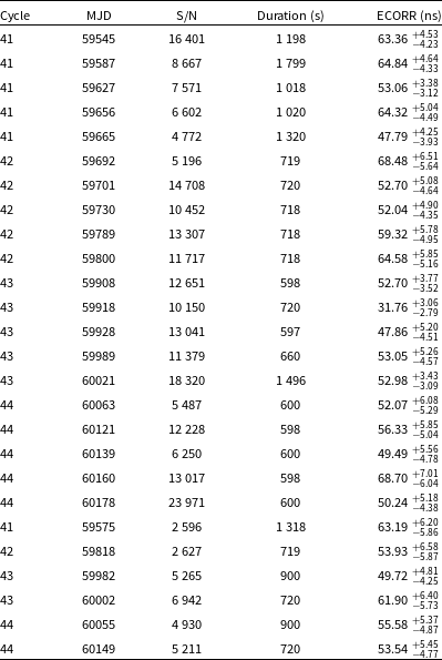
Table 1. Band 3 observations used in this work and their estimated jitter amplitudes. The first column lists the uGMRT observation cycle. The second column shows the date of the observations. The third column gives the integrated S/N ratios for this band obtained from the pdmp command of PSRCHIVE software package. The fourth column is the observation duration in seconds. The last column shows the ECORR value scaled to one hour and these values are plotted in Fig. 5. The bottom six epochs were selected to see the difference between Band 3 and 5 for the same epochs (see Section 3.3).
2. Observations and data processing
2.1. Observations
In this work, we have used the observations of PSR J0437 $-$
4715 conducted using uGMRT (Gupta et al. Reference Gupta2017) as a part of the InPTA experiment from the observation Cycle 41 to 44 (October 2021 to September 2023). The InPTA observations were carried out either using two sub-arrays of 10–15 antennae at Band 3 (300–500 MHz) and Band 5 (1 260–1 460 MHz), respectively or using the complete array set at Band 3. The voltages from individual antennas were added after compensating for the phase difference between different antennas to form phased array beams for both Band 3 and Band 5. This Nyquist sampled time series was converted to 1 024 frequency channels for Band 5 by taking a 2 048 point discrete Fourier Transform in the GMRT wideband backend. The Band 3 data were coherently dedispersed with the known DM of the pulsar to 128 frequency channels using a real-time pipeline (De & Gupta Reference De and Gupta2016) and sampled every 5.12
$-$
4715 conducted using uGMRT (Gupta et al. Reference Gupta2017) as a part of the InPTA experiment from the observation Cycle 41 to 44 (October 2021 to September 2023). The InPTA observations were carried out either using two sub-arrays of 10–15 antennae at Band 3 (300–500 MHz) and Band 5 (1 260–1 460 MHz), respectively or using the complete array set at Band 3. The voltages from individual antennas were added after compensating for the phase difference between different antennas to form phased array beams for both Band 3 and Band 5. This Nyquist sampled time series was converted to 1 024 frequency channels for Band 5 by taking a 2 048 point discrete Fourier Transform in the GMRT wideband backend. The Band 3 data were coherently dedispersed with the known DM of the pulsar to 128 frequency channels using a real-time pipeline (De & Gupta Reference De and Gupta2016) and sampled every 5.12 $\mu$
s. As the dual-band observation mode with the uGMRT allows the coherent dedispersion pipeline to be used only at one of the bands, the spectral time series was recorded with 1 024 channels for Band 5, in the regular phased array mode and sampled every 40.96
$\mu$
s. As the dual-band observation mode with the uGMRT allows the coherent dedispersion pipeline to be used only at one of the bands, the spectral time series was recorded with 1 024 channels for Band 5, in the regular phased array mode and sampled every 40.96 $\mu$
s. Given the low DM (2.6 pc cm
$\mu$
s. Given the low DM (2.6 pc cm $^{-3}$
) of the pulsar, the dispersion smear across a Band 5 channel is much smaller (
$^{-3}$
) of the pulsar, the dispersion smear across a Band 5 channel is much smaller ( $\sim$
2
$\sim$
2 $\mu$
s) than the sampling time used for Band 5, which is approximately equal to a phase bin across the profile. Thus, we do not expect significant aliasing to affect our results despite our observations being limited by the allowed observing mode and the lack of coherent dedispersion. The Julian dates and S/N ratio for each epoch used for our analysis can be found in Tables 1 and 2 for Band 3 and Band 5, respectively. More details about the InPTA observations and the associated observing strategy can be found in Tarafdar et al. (Reference Tarafdar2022) and Joshi et al. (Reference Joshi2022).
$\mu$
s) than the sampling time used for Band 5, which is approximately equal to a phase bin across the profile. Thus, we do not expect significant aliasing to affect our results despite our observations being limited by the allowed observing mode and the lack of coherent dedispersion. The Julian dates and S/N ratio for each epoch used for our analysis can be found in Tables 1 and 2 for Band 3 and Band 5, respectively. More details about the InPTA observations and the associated observing strategy can be found in Tarafdar et al. (Reference Tarafdar2022) and Joshi et al. (Reference Joshi2022).
2.2. Data processing
The processing of uGMRT pulsar observations was done using publicly available pulsar analysis tools described in this section. Here, we briefly summarise the data processing steps involved and the relevant software that was used in the analysis. The raw spectral time series was first reduced by converting it into RFI-mitigated partially folded profiles averaged every 10 s for each frequency channel using pinta Footnote a (Susobhanan et al. Reference Susobhanan2021) pipeline. The steps involved are as follows:
Table 2. Band 5 observations used in this work. The different columns refer to same parameters as in Table 1.
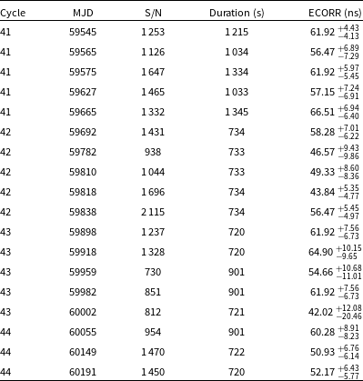
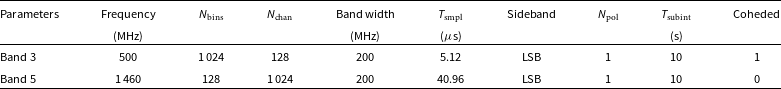
Table 3. Parameters used in pinta reduction. The first column is the local oscillator frequency of the observing band. The second column is the number of phase bins. The third column is the number of frequency channels. The fourth columns denotes the observation bandwidth. The fifth column is the sampling time used for observation. The sixth column is the sideband. The seventh column is number of polarisations. The eighth column is the duration of individual sub-integrations. The last column is whether the data has been coherently dedispersed (1) or not (0). More details on the description of these parameters can be found in Susobhanan et al. (Reference Susobhanan2021).
-
1. Convert the raw spectral data to filterbank format after removing impulsive and periodic RFI using algorithms developed for the uGMRT data with RFIClean Footnote b (Maan et al. Reference Maan, van Leeuwen and Vohl2021), which automatically remove periodic RFI in the Fourier domain.
-
2. The RFI-mitigated filterbank data were then folded for every frequency channel using an updated ephemeris of the pulsar every 10 s. This was done in the pipeline using DSPSR Footnote c (van Straten & Bailes Reference van Straten and Bailes2011). Each profile folded every 10 s represents a sub-integration in the observations consisting of all frequency channels that are recorded (128 and 1 024 in Band 3 and 5, respectively). These partially folded profiles were then written in the standard PSRFITS format for subsequent manipulation.
More details can be found in Susobhanan et al. (Reference Susobhanan2021) (and references therein). The pipeline parameters used are listed in Table 3. The subsequent analyses used tools provided by PSRCHIVE Footnote d software package (Hotan et al. Reference Hotan, van Straten and Manchester2004; van Straten et al. Reference van Straten, Demorest and Oslowski2012). For each epoch, an optimised S/N was obtained using the pdmp command provided by PSRCHIVE. The resulting S/N values were used for selecting the optimal observations analysed in this paper. We selected five epochs from each cycle for both Band 3 and Band 5, except for Band 5 in Cycle 44, since we did not have enough high S/N epochs. We also analysed six additional epochs, which have moderate S/N ratio in Band 3, and which were already selected for Band 5, to check the difference between Band 3 and 5 in the same epoch. In total, we analysed 26 epochs for Band 3 and 18 epochs for Band 5 as listed in Tables 1 and 2, respectively.
We first collapsed all the frequency channels in each PSRfits file into eight sub-bands after de-dispersing them, using the pam command of PSRCHIVE. Here, pam (which stands for Pulsar Archive Manipulator) is one of the commands within PSRCHIVE, which is widely used for post-processing partially folded profiles, such as dedispersion, collapsing the data over frequency and time and modifying the meta-data in the PSRFITS header. Next, the time-of-arrival (ToA) for each partially folded profile was obtained by cross-correlating these with a frequency resolved template. The template was formed by averaging all the sub-intergations using pam while preserving the eight sub-bands. These time-collapsed data were then dedispersed to obtain a final noise-free template using a wavelet filter implemented in psrsmooth command of PSRCHIVE. ToAs for every sub-integration in each observations were then obtained by cross-correlating the partially folded profiles with the noise-free template using the pat command of PSRCHIVE.
Finally, we obtained the timing residuals using the TEMPO2 Footnote e software packages for further analysis described in the next section. TEMPO2 is a package for pulsar timing analysis. This software compares the observed ToA with that predicted from a timing model, consisting of rotational, astrometric and binary parameters of a pulsar (Hobbs et al. Reference Hobbs, Edwards and Manchester2006; Edwards et al. Reference Edwards, Hobbs and Manchester2006). The sum of squares of the differences between the observed and predicted ToAs, called timing residuals, is minimised to obtain the best fit parameters of the pulsar. TEMPO2 is also used for simulating the TOAs using plug-ins provided in the software. We used TEMPO2 for simulations to estimate pulse jitter as explained in the next section. Before proceeding with the jitter measurements, we removed the TOAs with large uncertainties from a visual check. Finally, we carried out parameter fitting using only the spin frequency and DM, since the observations typically span 10 minutes in duration.
3. Jitter measurements
In this section, we first describe the noise models and the methods used to measure the jitter amplitudes. Thereafter, we present the results of jitter measurements.
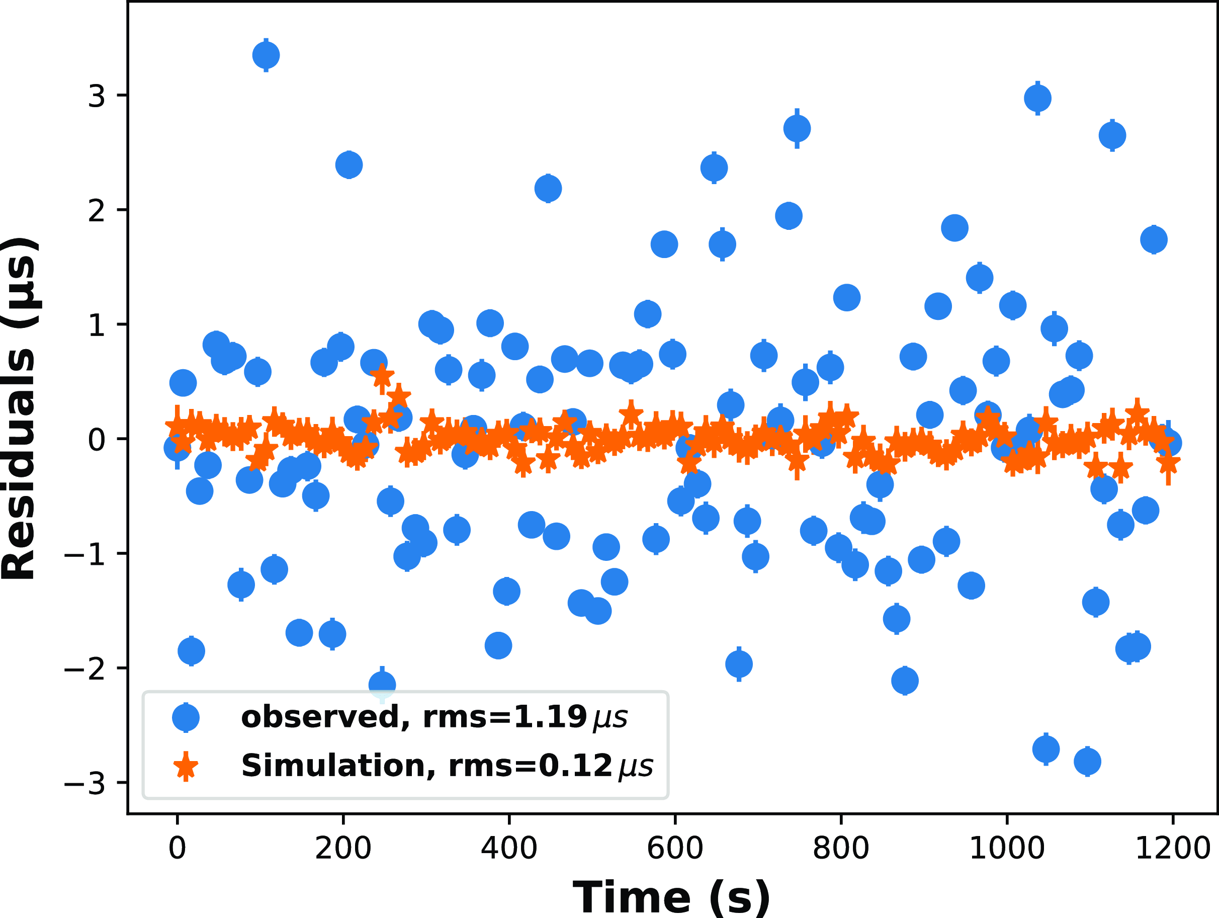
Figure 1. An example of the frequency-averaged timing residuals. The blue circles and orange stars denote the observed residuals obtained from 10 s sub-integrated profiles and residuals obtained with libstempo simulation, respectively (see the beginning of Section 3). The TOAs are obtained from Cycle 41 Band 3 observations for MJD 59545.
Traditionally, the jitter amplitudes have been estimated by computing the quadrature difference of the root-mean-square (rms) of frequency-averaged residuals, $\sigma_\textrm{obs}$
and the rms expected from the radiometer noise, (
$\sigma_\textrm{obs}$
and the rms expected from the radiometer noise, ( $\sigma_\textrm{rad}$
):
$\sigma_\textrm{rad}$
):
 \begin{equation} \sigma_\textrm{J}^2(T) = \sigma_\textrm{obs}^2(T) - \sigma_\textrm{rad}^2(T), \end{equation}
where T is the length of a sub-integration. We can estimate $\sigma_\textrm{rad}$
by considering the Gaussian noise expected from the observed TOA uncertainties. The simulated TOAs can be obtained using the fakepulsar method from the libstempo
Footnote f package, with the frequency-averaged TOAs and errors as input. fakepulsar is a plug-in within the TEMPO2 package. This particular plug-in enables the user to create simulated TOAs that fit a given timing model in the form of a given parameter file (Hobbs et al. Reference Hobbs, Edwards and Manchester2006). The timing model may correspond to either a real or a hypothetical pulsar. The addition of red and white noise is possible in this plug-in. The simulated timing residuals are encoded in an array with the same length as the total number of TOAs, which is filled with zeros. Then we can obtain the timing residuals containing radiometer noise by adding Gaussian noise using add_efac option. The rms of the timing residuals is denoted by
$\sigma_\textrm{rad}$
by considering the Gaussian noise expected from the observed TOA uncertainties. The simulated TOAs can be obtained using the fakepulsar method from the libstempo
Footnote f package, with the frequency-averaged TOAs and errors as input. fakepulsar is a plug-in within the TEMPO2 package. This particular plug-in enables the user to create simulated TOAs that fit a given timing model in the form of a given parameter file (Hobbs et al. Reference Hobbs, Edwards and Manchester2006). The timing model may correspond to either a real or a hypothetical pulsar. The addition of red and white noise is possible in this plug-in. The simulated timing residuals are encoded in an array with the same length as the total number of TOAs, which is filled with zeros. Then we can obtain the timing residuals containing radiometer noise by adding Gaussian noise using add_efac option. The rms of the timing residuals is denoted by $\sigma_\textrm{rad}$
. We obtain
$\sigma_\textrm{rad}$
. We obtain $\sigma_\textrm{rad}$
with 1 000 realisations and then calculate the jitter amplitude
$\sigma_\textrm{rad}$
with 1 000 realisations and then calculate the jitter amplitude $\sigma_\textrm{J}$
using Equation (1). One example of the frequency-averaged timing residuals and the simulated residuals is shown in Fig. 1. We can see that the frequency-averaged timing residuals have large fluctuations compared to the simulated timing residuals, suggesting that the remaining TOA fluctuation is due to pulse jitter. Jitter noise behaves like a white noise source and hence its amplitude scales inversely with the square root of the integration time, as shown below.
$\sigma_\textrm{J}$
using Equation (1). One example of the frequency-averaged timing residuals and the simulated residuals is shown in Fig. 1. We can see that the frequency-averaged timing residuals have large fluctuations compared to the simulated timing residuals, suggesting that the remaining TOA fluctuation is due to pulse jitter. Jitter noise behaves like a white noise source and hence its amplitude scales inversely with the square root of the integration time, as shown below.
 \begin{equation} \sigma_\textrm{J}(T_1) = \sigma_\textrm{J}(T_2) \sqrt{T_2/T_1}\end{equation}
For the rest of the paper, we report the jitter amplitudes, after rescaling them to 1 hour for the ease of comparison with previous studies.
3.1. Noise model
For the purpose of this study, we use Bayesian inference to estimate the jitter amplitude and used the traditional method described in the beginning of this section for crosscheck. In this subsection, we briefly describe the noise model used to estimate the jitter amplitude in this work. The following description is based on previous works (Lentati et al. Reference Lentati2014; van Haasteren & Vallisneri Reference van Haasteren and Vallisneri2014; Arzoumanian et al. Reference Arzoumanian2015; Srivastava et al. Reference Srivastava2023), where more details can be found.
The observed timing residuals can be defined in terms of an $N_\textrm{TOA}$
length vector, where
$N_\textrm{TOA}$
length vector, where $N_\textrm{TOA} = N_{\textrm{subint}} \times N_\textrm{subband}$
for a given observation, and can be modelled as a sum of various deterministic and stochastic noise sources. Since we are interested in the stochastic noise within a single epoch, we assume that the timing residual vector (
$N_\textrm{TOA} = N_{\textrm{subint}} \times N_\textrm{subband}$
for a given observation, and can be modelled as a sum of various deterministic and stochastic noise sources. Since we are interested in the stochastic noise within a single epoch, we assume that the timing residual vector ( $\delta$
t) can be fully described by the white noise term after removing the deterministic term. Therefore, the likelihood function can be written as follows:
$\delta$
t) can be fully described by the white noise term after removing the deterministic term. Therefore, the likelihood function can be written as follows:
 \begin{equation} L(\delta \textbf{t} | \theta) = \frac{1}{\sqrt{(2\pi)^{N_\textrm{TOA}} \det(\textbf{C}(\theta)) }}\exp\left(-\frac{1}{2}\delta\textbf{t}^T \textbf{C}(\theta)^{-1} \delta\textbf{t} \right),\end{equation}
where $\textbf{C}(\theta)$
is the covariance matrix and
$\textbf{C}(\theta)$
is the covariance matrix and $\theta$
is a set of parameters.
$\theta$
is a set of parameters.
In pulsar timing analysis, there are three parameters that are used to characterise white noise: EFAC, EQUAD, and ECORR. EFAC is a multiplicative scale factor that corrects for the underestimation of the TOA uncertainty that may be due to errors in calibration. EQUAD is a term that adds white noise in quadrature to represent the range of fluctuations beyond the TOA uncertainty. ECORR is similar to EQUAD, where white noise is again added in quadrature, but ECORR is uncorrelated in different time bins, but perfectly correlated at different frequencies. It represents the fluctuation of the TOA due to pulse profile variation. Therefore, ECORR corresponds to the jitter noise. EQUAD also corresponds to jitter as far as a single sub-band TOA is concerned. In this work, we use EFAC and EQUAD, when we estimate the jitter amplitude for each sub-banded TOA, and use EFAC and ECORR from the whole set of TOAs. We used the following three models to estimate the jitter amplitude:
-
Model I common EFAC and ECORR throughout the band.
-
Model II common EFAC throughout the band and different EQUAD for each sub-band.
-
Model III different EQUAD for each sub-band without EFAC.
In Model I, ECORR corresponds to the jitter amplitude for the given band. In Model II and III, we estimate the jitter for each sub-band. The aim of Model III is to eliminate any correlation between the sub-bands, since we used a common EFAC in Model II. The covariance matrix for each model can be written as follows:Footnote g
 \begin{align} &\textbf{Model, I} \quad \textbf{C}_{ij} = F ^2\sigma_{\textrm{TOA},i}^2\delta_{ij} + J^2 \delta_{t_i,t_j} \\[-29pt] \nonumber\end{align}
 \begin{align} &\textbf{Model, II} \quad \textbf{C}_{ij} = \left( F^2 \sigma_{\textrm{TOA},i}^2 + Q_{\nu_i}^2 \right) \delta_{ij}\\[-29pt] \nonumber \end{align}
 \begin{align} &\textbf{Model,III} \quad \textbf{C}_{ij} = \left( \sigma_{\textrm{TOA},i}^2 + Q_{\nu_i}^2 \right) \delta_{ij}\end{align}
where $\sigma_{{\textrm{TOA}},i}$
is the uncertainty of the ith TOA.
$\sigma_{{\textrm{TOA}},i}$
is the uncertainty of the ith TOA. $F,\, J$
refer to EFAC and ECORR, respectively.
$F,\, J$
refer to EFAC and ECORR, respectively. $Q_{\nu_i}$
denotes EQUAD for the ith sub-band. The index
$Q_{\nu_i}$
denotes EQUAD for the ith sub-band. The index $t_i$
represents the sub-integration of the ith TOA to incorporate ECORR in the same sub-integration. We used uniform prior distribution in [0.5, 5.0] for EFAC and log-uniform prior distribution in [-10.0, -5.0] for EQUAD and ECORR.
$t_i$
represents the sub-integration of the ith TOA to incorporate ECORR in the same sub-integration. We used uniform prior distribution in [0.5, 5.0] for EFAC and log-uniform prior distribution in [-10.0, -5.0] for EQUAD and ECORR.
3.2. Data analysis
To measure the jitter amplitude using Bayesian inference, we used the libstempo and the ENTERPRISE python packages (Ellis et al. Reference Ellis, Vallisneri, Taylor and Baker2020). libstempo is a Python wrapper to the tempo2 package. ENTERPRISE is a pulsar timing analysis software for pulsar noise analysis, GW searches and pulsar timing model analysis. We used the sub-banded TOAs and the corresponding par file as input. We then define the likelihood function depending on the Model I-III, from which the noise parameters are then estimated. We used the Markov Chain Monte Carlo (MCMC) sampler implemented in the PTMCMCSampler package (Ellis&van Haasteren Reference Ellis and van Haasteren2017) to sample the posterior and estimate the EFAC and ECORR or EQUAD. PTMCMCSampler is an acronym for Parallel Tempering Markov Chain Monte Carlo sampler and utilises an adaptive jump proposal mechanism by default, incorporating both standard and single-component Adaptive Metropolis (AM) as well as Differential Evolution (DE) jumps. Moreover, MPI (mpi4py) is employed to execute the parallel chains in this implementation. One example of such a posterior plot along with the marginalised posteriors for EFAC and ECORR is shown in Fig. 2.
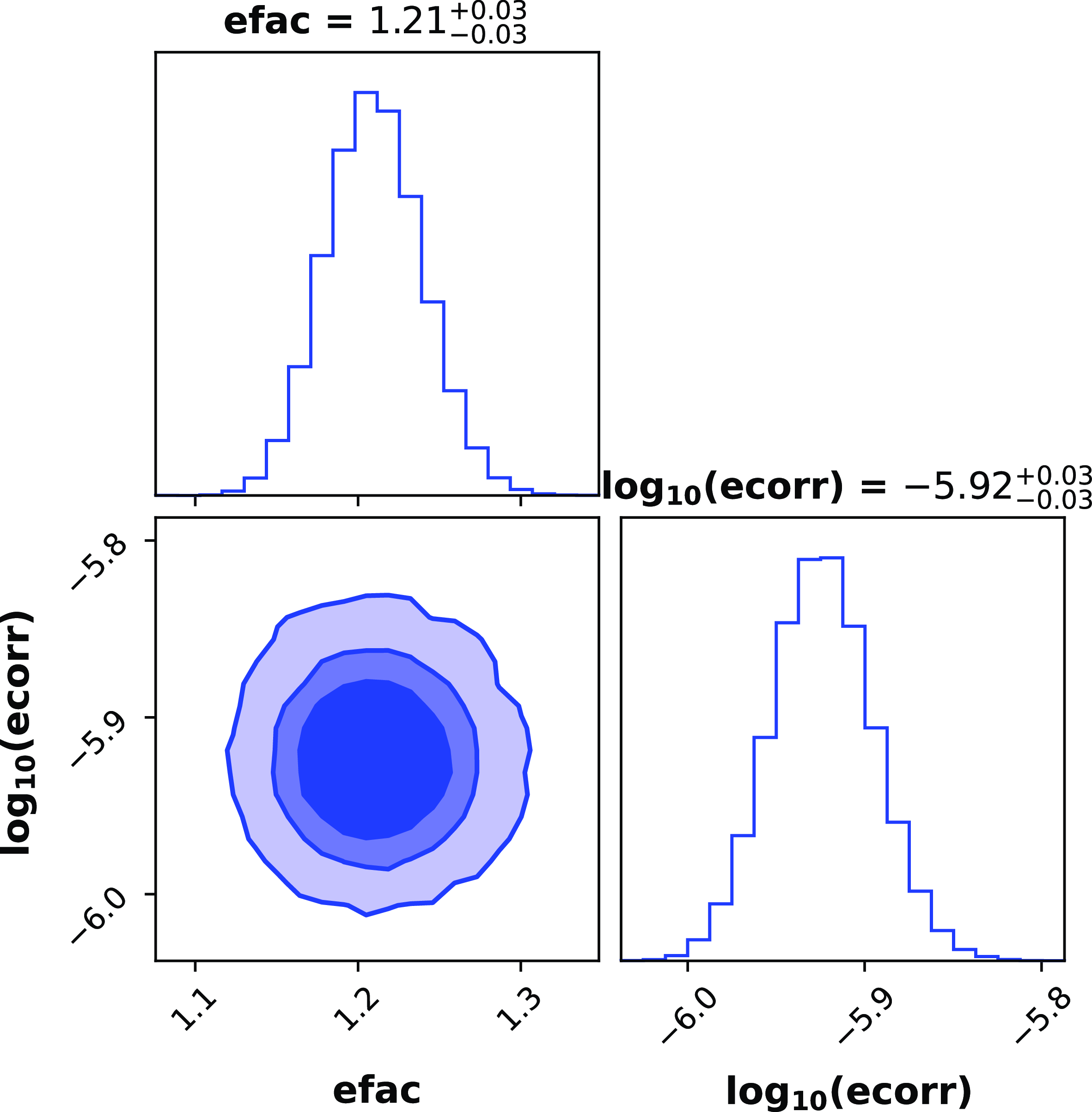
Figure 2. An example of the posterior distribution with 68%, 90%, 99% credible intervals of the Model I parameter estimation. The point estimates shown above the plots represent the median values and marginalised 68% credible intervals. The TOAs are obtained from Cycle 41 Band 3 observations on MJD 59545.
As mentioned at the beginning of Section 3, we rescale the estimated values of EQUAD and ECORR to one hour duration, using the same scaling relation as in Equation (2). However, in order to reaffirm whether they would follow the same relation as Equation (2), we recalculate ECORR for Model I by changing the sub-integration time to 20 and 40 seconds. The result is shown in Fig. 3, and we confirm that ECORR also follows the correct scaling law in accord with Equation (2). Although we do not have data for observation durations longer than one hour, we assume that the scaling law would hold even if the integration time is extended to one hour. Therefore, we scaled the jitter amplitude obtained by Bayesian analysis to one hour for ease of comparison with previous studies.
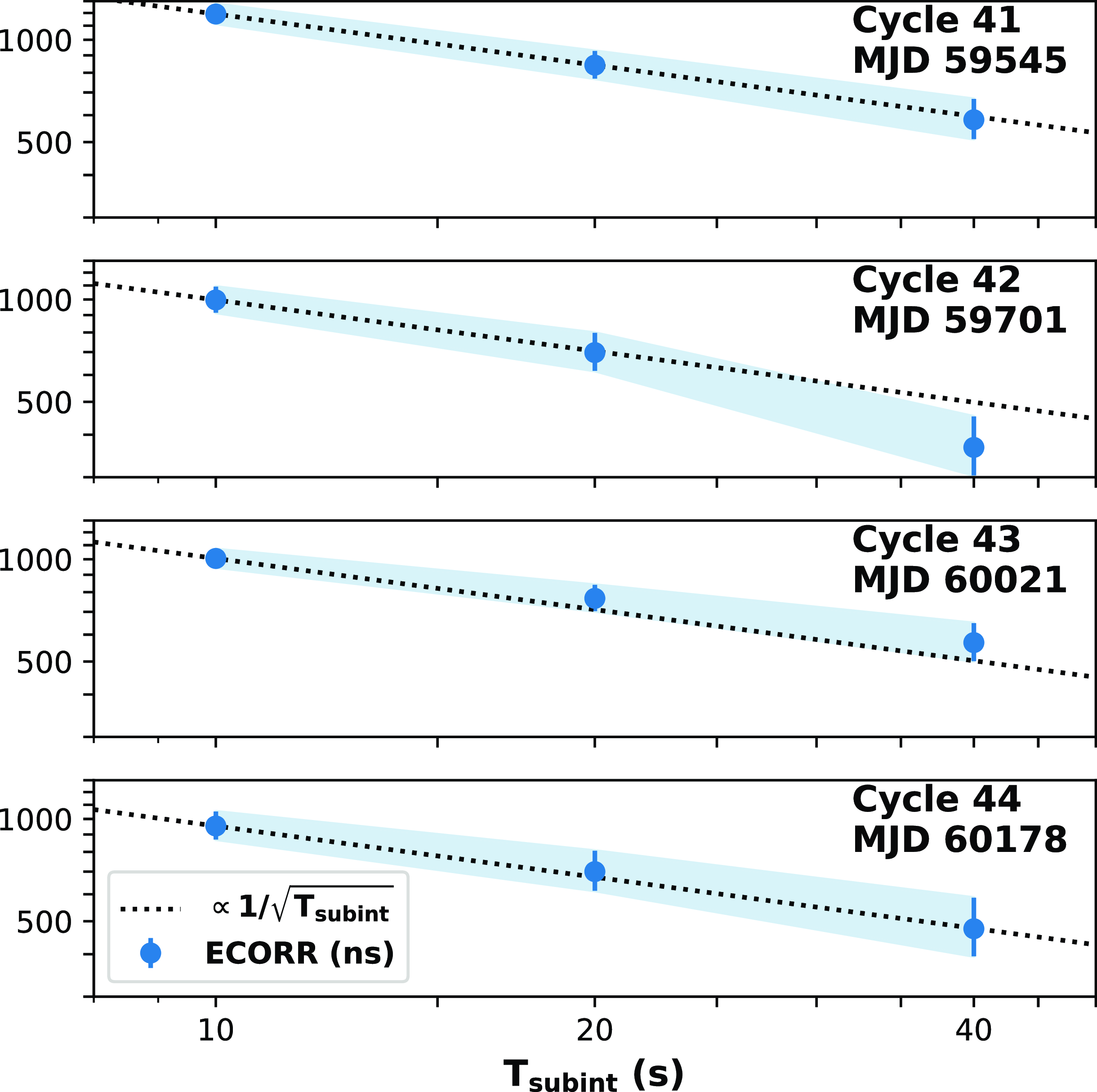
Figure 3. ECORR obtained with different sub-integration. Blue circles denote the ECORR values obtained from different sub-integration times. The black dotted lines shows the fit, which is proportional to the inverse square root of the sub-integration times.
As a consistency check, we also verify whether the ECORR values obtained with ENTERPRISE are consistent with the jitter amplitude obtained with the traditional method described in the beginning of this section (see Fig. 4). We find that all the $\sigma_\textrm{J }$
values agree with the ECORR values to within
$\sigma_\textrm{J }$
values agree with the ECORR values to within $1\sigma$
, thereby showing that our results are self-consistent.
$1\sigma$
, thereby showing that our results are self-consistent.
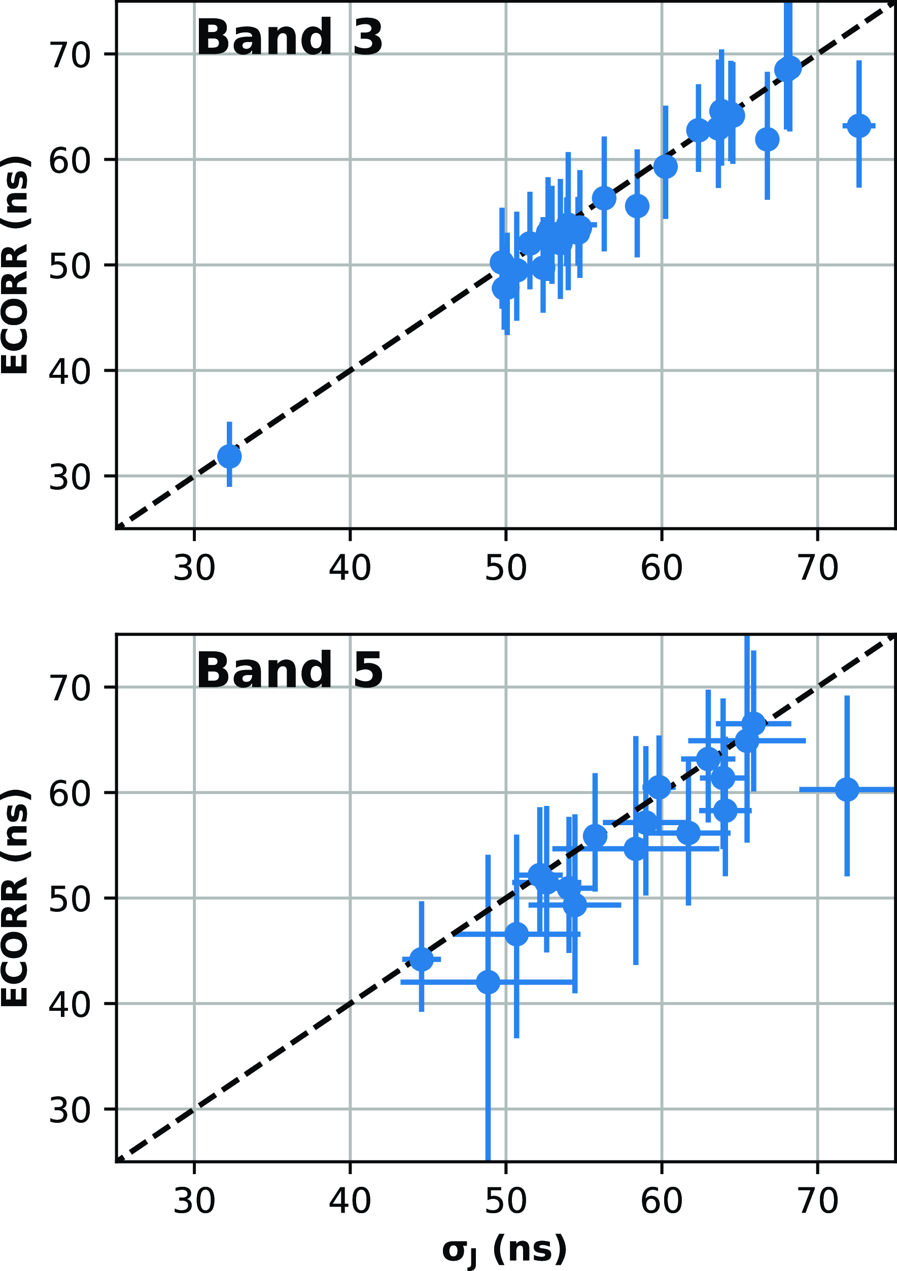
Figure 4. Comparison of jitter amplitudes obtained from Bayesian analysis and traditional method. The blue points denote jitter amplitude. The dashed black line represents the straight line given by $y=x$
. All values are scaled to 1 hour value using Equation (2).
$y=x$
. All values are scaled to 1 hour value using Equation (2).
3.3. Jitter amplitude within the band
Using the TOAs obtained by the method described in Section 2.2, we obtained ECORR values for all the selected epochs which are listed in Tables 1 and 2, for Model I of Section 3.1, which considers ECORR as a proxy for the jitter amplitude throughout the band. The resulting values of ECORR are rescaled to one hour and are listed in column 5 of Tables 1 and 2.
The rescaled ECORR values are plotted in Fig. 5 for each epoch. We estimate the weighted average of ECORR to be $53.2 \pm 0.9$
ns in Band 3 and
$53.2 \pm 0.9$
ns in Band 3 and $56.2 \pm 1.6$
ns in Band 5 from our observations. We find that our Band 5 result is consistent with P21. The jitter amplitude in S14 was reported for a single observation only. Though our weighted average value for Band 5 differs from that quoted in S14, the spread in our overall results ensures that we are in good agreement with S14 as well.
$56.2 \pm 1.6$
ns in Band 5 from our observations. We find that our Band 5 result is consistent with P21. The jitter amplitude in S14 was reported for a single observation only. Though our weighted average value for Band 5 differs from that quoted in S14, the spread in our overall results ensures that we are in good agreement with S14 as well.
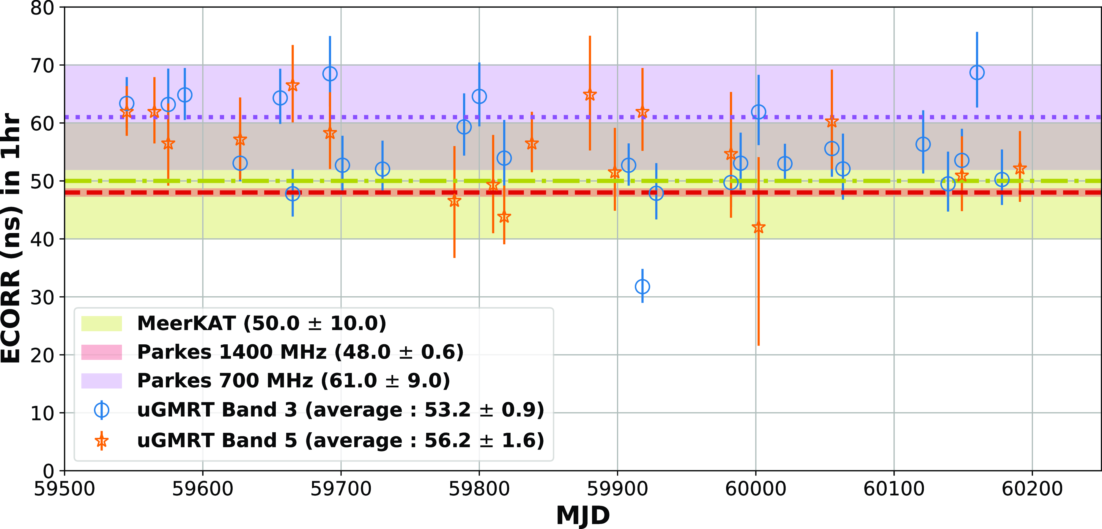
Figure 5. ECORR time series scaled to one hour obtained from Model I estimation. The blue circles and orange stars denote the ECORR values obtained from Band 3 and Band 5 observations, respectively. The purple shaded region and the dotted line show the results of MeerKAT observations (P21). The red shaded region and the dashed line and the yellow shaded region and dot-dashed line show the corresponding results for the Parkes observations (S14). Note that the values shown in the previous studies are not ECORR, but $\sigma_\textrm{J}$
defined by the Equation (1), which is measured by the traditional method described in the beginning of Section 3.
$\sigma_\textrm{J}$
defined by the Equation (1), which is measured by the traditional method described in the beginning of Section 3.
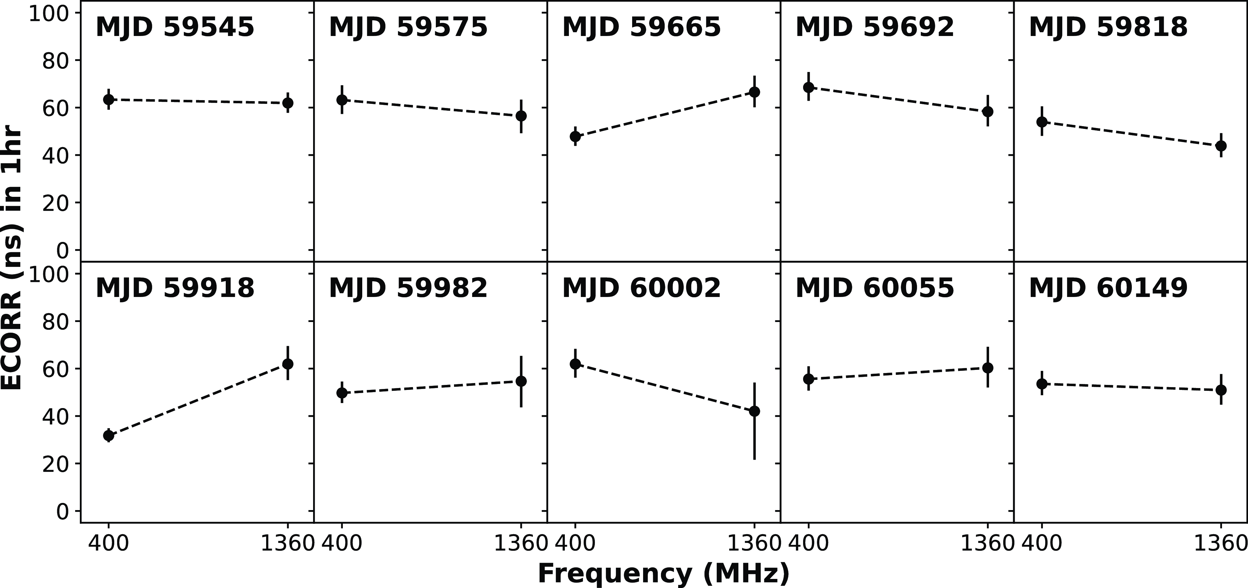
Figure 6. Comparison plots of ECORR for Band 3 and Band 5 for the same epoch obtained from Model I estimation.
Our results for ECORR at Band 3 are the first jitter measurements calculated for PSR J0437 $-$
4715 below 700 MHz. Therefore, we do not have previous studies to directly compare our results. The frequency dependence suggested by S14 and P21 point to a higher jitter at lower frequencies. The results we derive are, however, not in agreement with this conclusion since we find that ECORR at Band 3 is consistent with that seen in Band 5. Also, we see that the weighted average of the jitter amplitude at Band 3 is slightly lower than that of Band 5. We calculated the weighted average again after excluding the epoch corresponding to MJD 59918, since it is likely to be an outlier as it is strongly affected by scintillation. This gave a new weighted average value of jitter at Band 3, equal to
$-$
4715 below 700 MHz. Therefore, we do not have previous studies to directly compare our results. The frequency dependence suggested by S14 and P21 point to a higher jitter at lower frequencies. The results we derive are, however, not in agreement with this conclusion since we find that ECORR at Band 3 is consistent with that seen in Band 5. Also, we see that the weighted average of the jitter amplitude at Band 3 is slightly lower than that of Band 5. We calculated the weighted average again after excluding the epoch corresponding to MJD 59918, since it is likely to be an outlier as it is strongly affected by scintillation. This gave a new weighted average value of jitter at Band 3, equal to $55.47 \pm 0.94$
ns. Therefore, even after removing the outlier, the jitter in Band 3 is consistent with that in Band 5 within
$55.47 \pm 0.94$
ns. Therefore, even after removing the outlier, the jitter in Band 3 is consistent with that in Band 5 within $1\sigma$
. One possible reason that the jitter in Band 3 is not so large could be due to epoch to epoch variations, since we are comparing different epochs. In Fig. 6, we plot the ECORR values for Band 3 and Band 5 from same epochs, for comparing their behaviour. We see that while there are some epochs where the jitter in Band 3 is larger, there are also epochs where the jitter values at Band 3 are the same or smaller. From our whole band jitter (ECORR) estimates, we conclude that it is not possible to say with certainty whether the jitter is larger or smaller at lower frequencies than at higher frequencies.
$1\sigma$
. One possible reason that the jitter in Band 3 is not so large could be due to epoch to epoch variations, since we are comparing different epochs. In Fig. 6, we plot the ECORR values for Band 3 and Band 5 from same epochs, for comparing their behaviour. We see that while there are some epochs where the jitter in Band 3 is larger, there are also epochs where the jitter values at Band 3 are the same or smaller. From our whole band jitter (ECORR) estimates, we conclude that it is not possible to say with certainty whether the jitter is larger or smaller at lower frequencies than at higher frequencies.
We see that there is a large scatter in the Band 3 jitter estimates. On investigating the Band 3 pulsar profiles in the frequency domain, we find that this scatter in the jitter values might be caused by the scintillation present in many profiles. Further, we notice that in this band, the S/N varies significantly with frequency as well as from epoch to epoch, which again can possibly be explained by the presence of interstellar scintillation in the data. This may have caused the failure in measuring the fluctuations of the timing residuals for some of the sub-bands which have low-S/N, thereby resulting in higher jitter estimates. As a result, we further scrutinise the Band 3 data for further insights on the nature of jitter.
3.4. Intra-band frequency dependence of Jitter
In Section 3.3, we have demonstrated that the jitter estimates at low frequency may be affected by scintillation. This prompted us to look at the sub-banded data to get additional insight into the nature of jitter in the different frequency channels of Band 3. In this analysis, we estimate EQUAD for each sub-band using Model II and III from the 20 highest S/N epochs listed in Table 1. EQUAD is used to account for the unaccounted (besides telescope noise) noise in the TOA uncertainty, and it corresponds to the jitter amplitude estimated using the traditional method described in the beginning of Section 3 (S14; P21).
Learning from our experience in Section 3.3, where low S/N hindered us from getting accurate jitter estimates at Band 3, we obtain credible EQUAD values by first calculating the sub-banded S/N and then adopting EQUAD values from only those high S/N observations that lie above a given threshold. The sub-banded S/N is defined as follows:
 \begin{equation} \textrm{S/N}_{\textrm{sub}} = \frac{\sum_{i, j} I_{i,j}}{\sigma_I}, \end{equation}
where $I_{i,j}$
is the intensity of
$I_{i,j}$
is the intensity of $i{\rm th}$
phase bin and
$i{\rm th}$
phase bin and $j{\rm th}$
sub-integration in a certain sub-band,
$j{\rm th}$
sub-integration in a certain sub-band, $\sigma_I=\sqrt{\sum_{i} \sigma_{I, i}^2}$
is the rms of the intensity in a certain sub-band, and
$\sigma_I=\sqrt{\sum_{i} \sigma_{I, i}^2}$
is the rms of the intensity in a certain sub-band, and $\sigma_{I,i}$
is the rms of the intensity in the
$\sigma_{I,i}$
is the rms of the intensity in the $i{\rm th}$
phase bin. We used the median value of the S/N_sub as our threshold, which is equal to S/N_sub = 2 606.
$i{\rm th}$
phase bin. We used the median value of the S/N_sub as our threshold, which is equal to S/N_sub = 2 606.
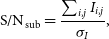
The results from parameter estimation for Model II and III are shown in Fig. 7, which clearly show a tendency for an increase in EQUAD with frequency for both the models. To reaffirm this quantitatively, we performed a Bayesian regression and estimated the slope (a), and EQUAD at 400 MHz ( $Q_{400}$
) using the emcee
Footnote h MCMC sampler (Foreman-Mackey et al. Reference Foreman-Mackey, Hogg, Lang and Goodman2013). The emcee package uses an affine invariant Affine Invariant Markov chain Monte Carlo Ensemble sampler using the algorithm in Goodman &Weare (Reference Goodman and Weare2010). We used the following regression model:
$Q_{400}$
) using the emcee
Footnote h MCMC sampler (Foreman-Mackey et al. Reference Foreman-Mackey, Hogg, Lang and Goodman2013). The emcee package uses an affine invariant Affine Invariant Markov chain Monte Carlo Ensemble sampler using the algorithm in Goodman &Weare (Reference Goodman and Weare2010). We used the following regression model:
 \begin{equation} y = a (f-400) + Q_{400} \end{equation}
where f is the frequency. After performing the regression, we randomly sampled 500 values from the posterior distribution of a and $Q_{400}$
, and then the results using these values are depicted as the blue and orange regions in Fig. 7. We see that the lines have a positive slope implying an increase in EQUAD with frequency, a trend that is opposite to that of S14 and P21.
$Q_{400}$
, and then the results using these values are depicted as the blue and orange regions in Fig. 7. We see that the lines have a positive slope implying an increase in EQUAD with frequency, a trend that is opposite to that of S14 and P21.
Figure 7. Sub-banded EQUAD scaled to one hour obtained from Model II and III estimation for the sub-bands which had the $\textrm{S/N}_\textrm{sub}$
above the threshold value. The blue circles and orange stars represent the sub-banded EQUAD value of Model II (with EFAC) and III (without EFAC), respectively. The orange stars have been offset by 5 MHz to the right for clarity. The blue and orange shaded lines are from 500 random lines obtained from the posterior distribution of Bayesian regression. The reduced
$\textrm{S/N}_\textrm{sub}$
above the threshold value. The blue circles and orange stars represent the sub-banded EQUAD value of Model II (with EFAC) and III (without EFAC), respectively. The orange stars have been offset by 5 MHz to the right for clarity. The blue and orange shaded lines are from 500 random lines obtained from the posterior distribution of Bayesian regression. The reduced $\chi^2$
of the best-fit lines are equal to 4.8 for Model II and 1.7 for Model III.
$\chi^2$
of the best-fit lines are equal to 4.8 for Model II and 1.7 for Model III.
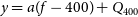
The posterior distributions of a and $Q_{400}$
are shown in Figs. 8 and 9, respectively. These plots show that the slopes have a positive value with significance of about
$Q_{400}$
are shown in Figs. 8 and 9, respectively. These plots show that the slopes have a positive value with significance of about $15\sigma$
. The plots also list the value of
$15\sigma$
. The plots also list the value of $Q_{400}$
, or the jitter amplitude at 400 MHz, which is about
$Q_{400}$
, or the jitter amplitude at 400 MHz, which is about $54.14^{+0.66}_{-0.68}$
ns, in Model II and
$54.14^{+0.66}_{-0.68}$
ns, in Model II and $58.83^{+0.63}_{-0.63}$
ns, in Model III.
$58.83^{+0.63}_{-0.63}$
ns, in Model III.
Figure 8. Posterior distributions with 68%, 90%, 99% credible intervals for the parameters fitted using Model II in Fig. 7. The point estimates shown above the plots represent the median values and marginalised 68 % credible intervals.
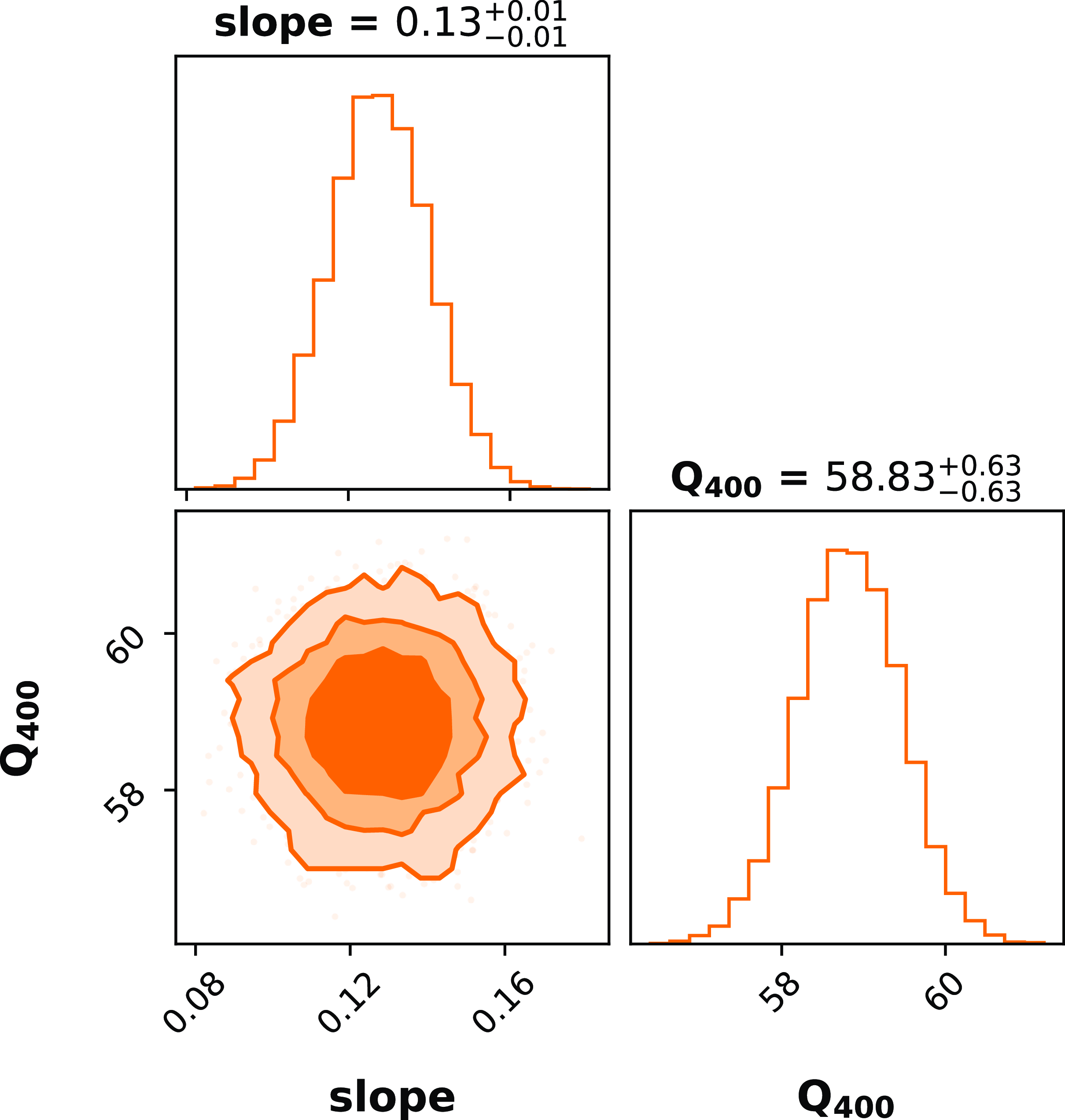
Figure 9. Posterior distributions with 68%, 90%, 99% credible intervals for the parameters fitted using Model III in Fig. 7. The point estimates shown above the plots represent the median values and marginalised 68 % credible intervals.
3.5. Jitter and the DM variations
P21 raised the concern of the jitter being the limiting factor in the DM precision measurements from shorter duration observations in all MSPs and suggested that it can only be overcome by longer integrations, based on their analysis in the high-frequency regime. We investigated the effect of jitter on the DM precision in the low-frequency regime (300–500 MHz) by studying the timing residuals and obtaining the DM uncertainties for 10 second sub-integrations from a 20 minute observation done at the uGMRT.
We measured the timing residuals from each of its 10 second sub-integrations, where each sub-integration is divided into eight frequency channels. We plot in Fig. 10, a small subset of the post-fit timing residuals derived from the TOAs. These are plotted serially in time, with each TOA observation being 10 seconds long. The residuals are colour coded for a given frequency sub-band (as mentioned in Fig. 10). There seems to be a dependence of the timing residuals on frequency on a 10 second timescale, which may be due to the frequency dependence of DM. The dependence of the TOA on frequency at Band 3 is, however, not as strong as that shown for the high-frequency regime in P21. This probably implies a smaller spread in DM at Band 3 compared to that in the higher frequency band reported in P21.
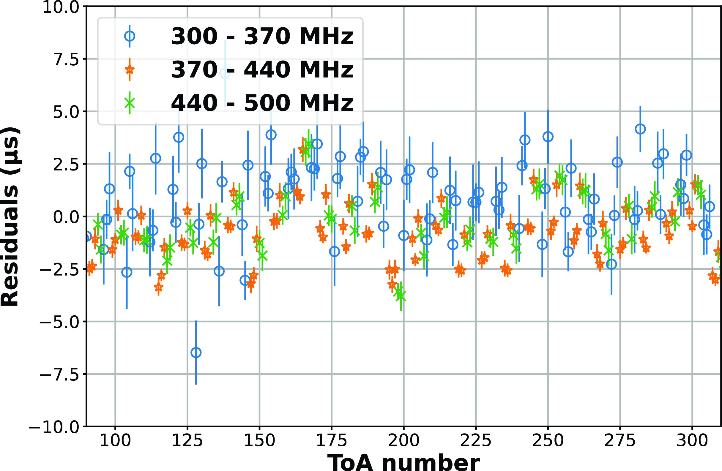
Figure 10. A subset of the ‘Post-fit timing residuals’ of PSR J0437 $-$
4715 estimated using 10 second sub-integrated profiles with each having eight frequency channels. The TOAs are subdivided and colour coded as three sets based on the frequency sub-band as shown in the figure. These residuals are plotted serially against the TOA numbers, to check for any potential frequency dependence and its variation for each TOA set in the plotted subset. The complete observation spanned 20 minutes, and only a subset is plotted in this figure for clarity.
$-$
4715 estimated using 10 second sub-integrated profiles with each having eight frequency channels. The TOAs are subdivided and colour coded as three sets based on the frequency sub-band as shown in the figure. These residuals are plotted serially against the TOA numbers, to check for any potential frequency dependence and its variation for each TOA set in the plotted subset. The complete observation spanned 20 minutes, and only a subset is plotted in this figure for clarity.
To explore this, we measured the DM values independently from the TOAs of each 10 second sub-integration of the observation. From this, we estimated the median DM to be $2.64386$ $\textrm{cm}^{-3} \,\textrm{pc}$
and a standard deviation of
$\textrm{cm}^{-3} \,\textrm{pc}$
and a standard deviation of $8.4 \times 10^{-5} \textrm{cm}^{-3} \,\textrm{pc}$
. This is shown graphically in Fig. 11. We conclude that the scatter in DM is less at Band 3 compared to higher frequency bands (see figure 4 of P21).
$8.4 \times 10^{-5} \textrm{cm}^{-3} \,\textrm{pc}$
. This is shown graphically in Fig. 11. We conclude that the scatter in DM is less at Band 3 compared to higher frequency bands (see figure 4 of P21).
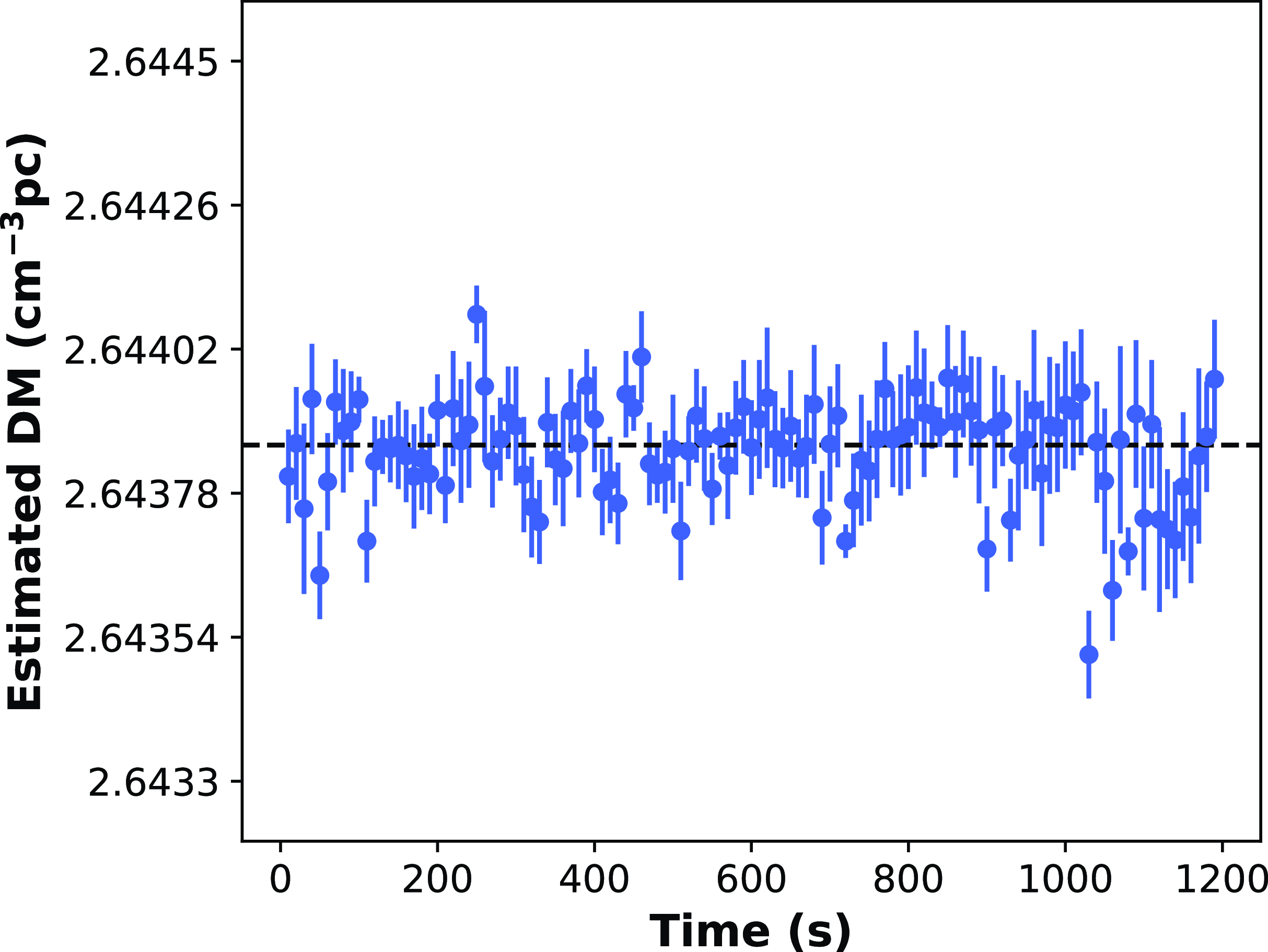
Figure 11. The estimated DM values for each 10 second sub-integration from psrfits to the timing residuals shown in Fig. 10. The horizontal dotted line represents the median estimated DM value of 2.64386 $\textrm{cm}^{-3} \,\textrm{pc}$
Further, to understand the effect of jitter on the DM precision measurements and to get one more independent check on the DM estimation from observations alone, we use the following equation to derive the resultant error in the DM estimation:
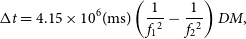 \begin{equation} {\Delta t}= 4.15 \times 10^6 (\textrm{ms}) \left(\frac{1}{ {{f_1}{^ 2}} } - \frac{1} { {{f_2}{^ 2}} }\right)DM,\end{equation}
where $\Delta t$
is the delay in TOAs at the two observing frequencies,
$\Delta t$
is the delay in TOAs at the two observing frequencies, $f_1$
and
$f_1$
and $f_2$
.
$f_2$
.
As shown in Sections 3.3 and 3.4, the pulse jitter is frequency dependent. In Band 3, it has a larger value at higher frequencies, as can be seen from Fig. 7. To estimate the contribution of pulse jitter in the DM precision, we calculate jitter for a 10 second sub-integration at the two extreme frequencies of our observation, namely 311 and 486 MHz, using Equation (2). We find the jitter estimate for a 10 second observation to be 1 121.69 and 1 287.87 ns for 311 and 486 MHz, respectively. Assuming the error in TOAs to be due to jitter alone, we infer the DM error to be $\sim 6.7\times10^{-5} \textrm{cm}^{-3} \,\textrm{pc}$
which is marginally less than our observationally derived error of
$\sim 6.7\times10^{-5} \textrm{cm}^{-3} \,\textrm{pc}$
which is marginally less than our observationally derived error of ${\sim}8.4\times10^{-5}\textrm{cm}^{-3} \,\textrm{pc}$
. However, the error in the TOAs is not due to jitter alone and the other major factor which contributes to this error is the telescope noise. This observation on which the analysis is done is a high S/N observation, with a S/N of at least 1 000 for each 10 second sub-integration. Hence in this case, the telescope noise is about
${\sim}8.4\times10^{-5}\textrm{cm}^{-3} \,\textrm{pc}$
. However, the error in the TOAs is not due to jitter alone and the other major factor which contributes to this error is the telescope noise. This observation on which the analysis is done is a high S/N observation, with a S/N of at least 1 000 for each 10 second sub-integration. Hence in this case, the telescope noise is about $\sim$ $10^{-6}$
, which is slightly less than the jitter noise of
$10^{-6}$
, which is slightly less than the jitter noise of $\sim$ $1.71\times10^{-6}$
, and therefore, we can assert that the error in TOAs is dominated by the jitter noise in high S/N but lower integration time observations. Including the contribution of telescope noise in the aforementioned analysis increases the DM error marginally to be around
$1.71\times10^{-6}$
, and therefore, we can assert that the error in TOAs is dominated by the jitter noise in high S/N but lower integration time observations. Including the contribution of telescope noise in the aforementioned analysis increases the DM error marginally to be around $7.8\times10^{-5} \textrm{cm}^{-3} \,\textrm{pc} $
. Thus, our two independent analyses for the DM uncertainties are in good agreement with each other, thereby providing confidence in our inferences for the jitter measurement and its effect on the DM precision.
$7.8\times10^{-5} \textrm{cm}^{-3} \,\textrm{pc} $
. Thus, our two independent analyses for the DM uncertainties are in good agreement with each other, thereby providing confidence in our inferences for the jitter measurement and its effect on the DM precision.
4. Discussion
4.1. Origin of the frequency dependence in jitter
Our analysis of the high S/N Band 3 observations of PSR J0437 $-$
4715 reveals a positive correlation of jitter with frequency, as shown in Section 3.4. Therefore, we find an opposite trend than that suggested by S14 and P21 for their higher frequency observations. It could be due to two possible reasons. One is due to the possibility that the pulse profile is more stable at lower frequencies than at higher frequencies in Band 3. This is because jitter is caused by the pulse profile variation in the pulse-to-pulse scale. And second, there seems to exist a turnover frequency region at which the jitter trend reverses. This region seems to exist between 500 and 900 MHz, probably around 700 MHz.
$-$
4715 reveals a positive correlation of jitter with frequency, as shown in Section 3.4. Therefore, we find an opposite trend than that suggested by S14 and P21 for their higher frequency observations. It could be due to two possible reasons. One is due to the possibility that the pulse profile is more stable at lower frequencies than at higher frequencies in Band 3. This is because jitter is caused by the pulse profile variation in the pulse-to-pulse scale. And second, there seems to exist a turnover frequency region at which the jitter trend reverses. This region seems to exist between 500 and 900 MHz, probably around 700 MHz.
The existence of a turnover frequency region at which jitter behaviour changes can possibly have two interpretations, which we outline below. The first interpretation comes from the self-absorption effect in the pulsar magnetosphere. It has been shown that the high-frequency radio emission from the pulsar comes from regions closer to its surface, while the low-frequency emission comes from regions farther from the surface (Komesaroff Reference Komesaroff1970; Cordes Reference Cordes1978). This is called the radius-to-frequency mapping (RFM). Of the many pulsars studied, most show this trend but there are a few some exceptions (Posselt et al. Reference Posselt2021). Based on the RFM studies, we can say that since the distance of propagation through the emission region is shorter for lower frequencies, these are less sensitive to the self-absorption effects, thereby resulting in more stable profiles than those at higher frequencies. If this is true, the turnover frequency of the jitter amplitude could be related to the spectral turnover of the pulsar flux density. However, Lee et al. (Reference Lee2022) reported two turnover frequencies of the flux density for PSR J0437 $-$
4715, which are
$-$
4715, which are $\sim$ $285 \,\textrm{MHz}$
and
$285 \,\textrm{MHz}$
and $\sim$ $1\,900 \,\textrm{MHz}$
. This is therefore, not supporting our ansatz for the change in the jitter trend. In any case, it remains to be seen how jitter behaves around these two frequencies. A holistic mapping of the jitter trend over the full span of frequency bands will probably provide a clearer picture.
$1\,900 \,\textrm{MHz}$
. This is therefore, not supporting our ansatz for the change in the jitter trend. In any case, it remains to be seen how jitter behaves around these two frequencies. A holistic mapping of the jitter trend over the full span of frequency bands will probably provide a clearer picture.
The second possibility comes from the profile evolution studies. The analysis in S14 and P21 suggested that the possible reason for the smaller jitter at higher frequencies is due to narrower pulses and the larger modulation of the main pulse component at those frequencies. However, our jitter trend is opposite to their results. PSR J0437 $-$
4715 seems to have a narrow central component in its profile above 700 MHz (Dai et al. Reference Dai2015). Comparing 1 400 MHz observations with 327 MHz observations for this pulsar, we find relatively more stable precursor and postcursor components at lower frequency (Osłowski et al. Reference Osłowski, van Straten, Hobbs and Bailes2014; Vivekanand et al. Reference Vivekanand, Ables and McConnell1998). We notice that the pulse profiles show more significant precursor and postcursor components in our Band 3 observations as well (see Fig. 12). This leads us to posit that the reason for the smaller jitter at lower frequencies at Band 3 is due to the fact that these precursor and postcursor components are more stable, and hence they moderate the fluctuations in the TOAs by the central (main) component. To investigate this further we need to study the phase-resolved modulation index of single pulses, which may help resolve this issue. Hence, it will be worth revisiting single-pulse studies of PSR J0437
$-$
4715 seems to have a narrow central component in its profile above 700 MHz (Dai et al. Reference Dai2015). Comparing 1 400 MHz observations with 327 MHz observations for this pulsar, we find relatively more stable precursor and postcursor components at lower frequency (Osłowski et al. Reference Osłowski, van Straten, Hobbs and Bailes2014; Vivekanand et al. Reference Vivekanand, Ables and McConnell1998). We notice that the pulse profiles show more significant precursor and postcursor components in our Band 3 observations as well (see Fig. 12). This leads us to posit that the reason for the smaller jitter at lower frequencies at Band 3 is due to the fact that these precursor and postcursor components are more stable, and hence they moderate the fluctuations in the TOAs by the central (main) component. To investigate this further we need to study the phase-resolved modulation index of single pulses, which may help resolve this issue. Hence, it will be worth revisiting single-pulse studies of PSR J0437 $-$
4715 with our high-sensitivity, wideband observations, which will be defered to a future paper.
$-$
4715 with our high-sensitivity, wideband observations, which will be defered to a future paper.
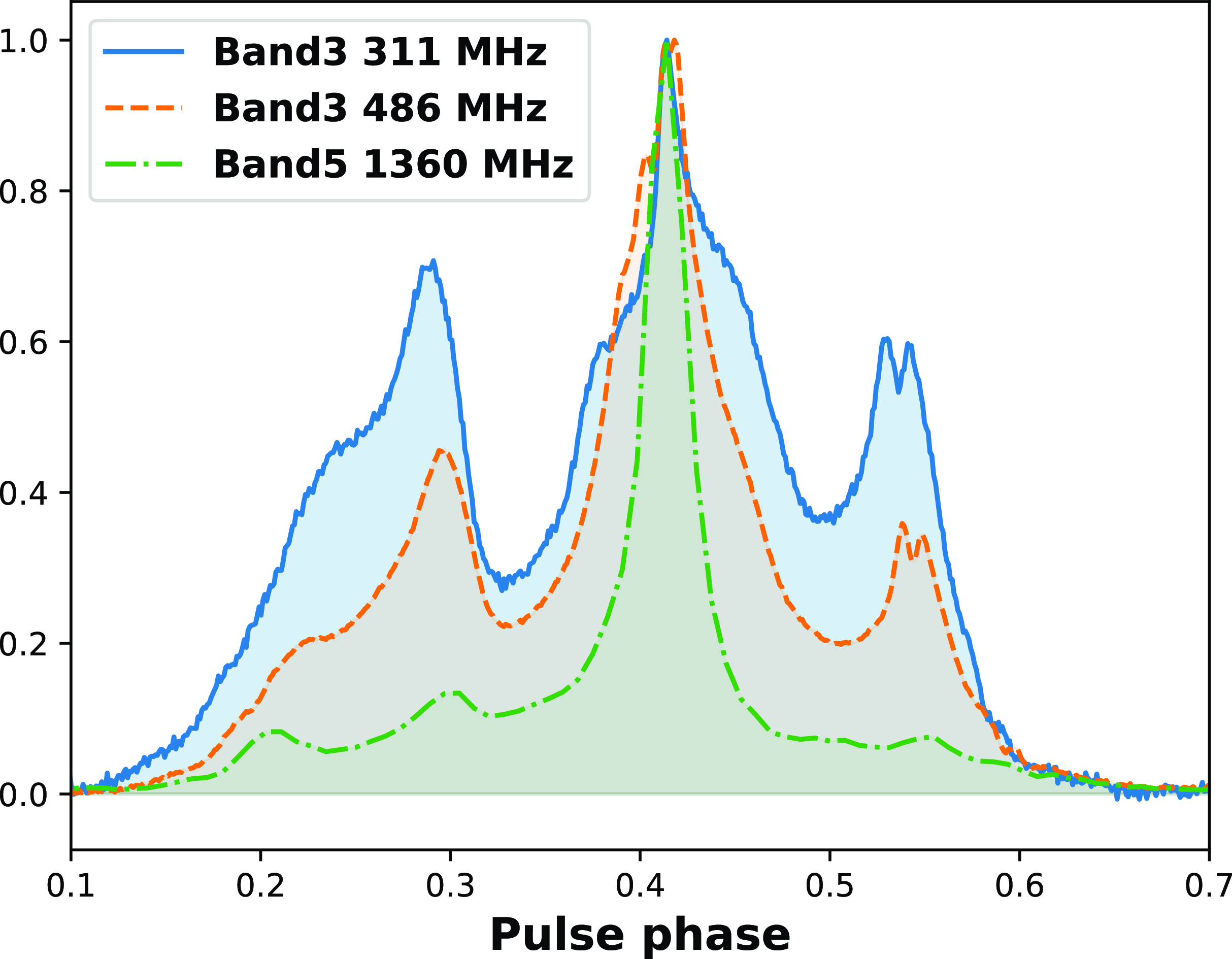
Figure 12. The integrated pulse profile of PSR J0437 $-$
4715 at different frequencies. Intensities are normalised. The data used for this plot were obtained from Cycle 41 observation on MJD 59545.
$-$
4715 at different frequencies. Intensities are normalised. The data used for this plot were obtained from Cycle 41 observation on MJD 59545.
4.2. Effect of jitter on the DM precision measurements
From our analysis, in Section 3.5, we see that the DM precision is limited by jitter noise for high S/N observations on short timescales. Further, if we extrapolate the results from P21, it would indicate that we cannot get high precision DM just by going to lower frequencies. However, our analysis suggests otherwise, and it might be possible to get even better precision DMs by going to lower frequencies ( $\sim$
100 MHz). Though the possibility of low frequency giving better DM precision is supported by our analysis at Band 3, it remains to be seen observationally what trend is followed by pulse jitter at that frequency regime.
$\sim$
100 MHz). Though the possibility of low frequency giving better DM precision is supported by our analysis at Band 3, it remains to be seen observationally what trend is followed by pulse jitter at that frequency regime.
Further, our analysis in tandem with P21 suggests that it is not possible to get DM precision measurements using observations at two (high and low) frequencies only. This is because the DM will depend on the jitter coming from both the observed frequencies; and it is entirely possible that those two frequencies may show entirely opposite trends in jitter (e.g. at Band 3 and Band 5). For more precise estimates of jitter, we need to be able to extrapolate over multiple bands in a frequency resolved manner, since different frequency bands are likely to give different estimate for order of precision.
A comprehensive understanding of the pulse-jitter behaviour over different frequency bands and its effect on DM is warranted for better precision pulsar timing. It also remains to be seen what trend in jitter is followed by different pulsars at different frequency bands. Our data show lower jitter and hence more precise DMs at lower frequencies (than higher frequencies). However, low-frequency studies of other pulsars are required to see if this trend is universal. It is very well possible that the trend is opposite for other pulsars and this is a subject of a subsequent analysis.
5. Conclusions
In this work, we present the first ever jitter measurements of PSR J0437 $-$
4715 in the low-frequency region (300–500 MHz), using Band 3 wideband observations obtained as a part of the InPTA experiment. We were able to estimate the jitter values in both Band 3 and 5 using Bayesian inference. For Band 5, our jitter measurements are in agreement with the previous studies; (S14 and P21). In this band, we estimate the weighted average of jitter to be
$-$
4715 in the low-frequency region (300–500 MHz), using Band 3 wideband observations obtained as a part of the InPTA experiment. We were able to estimate the jitter values in both Band 3 and 5 using Bayesian inference. For Band 5, our jitter measurements are in agreement with the previous studies; (S14 and P21). In this band, we estimate the weighted average of jitter to be $56.2 \pm 1.6$
ns. Our Band 3 weighted average value for the jitter is
$56.2 \pm 1.6$
ns. Our Band 3 weighted average value for the jitter is $53.2 \pm 0.9$
ns, which is lower than that in Band 5. Therefore, we see a positive correlation in the frequency dependence of jitter at low frequencies in the 300–500 MHz range. To explore the reason for this, we measured the jitter amplitude in each frequency sub-band also, using sub-banded TOAs from Band 3 observations. The results from the sub-banded data reaffirmed the positive correlation of the jitter amplitude with frequency. Therefore, positive correlation of the jitter with frequency in our low-frequency (Band 3) analysis in tandem with the negative correlation of jitter with frequency in high-frequency analysis by S14 and P21 suggests the existence of a turnover frequency region for the jitter amplitude. This turnover region probably lies somewhere between 500 and 700 MHz and this explains why our jitter amplitude of Band 3 is not as large as expected from previous high-frequency studies alone. It would be interesting to explore this turnover region further and this turnover frequency could possibly be determined by the uGMRT Band 4 (550–750 MHz) observations, or the next generation, high-sensitivity telescopes, such as the SKA.
$53.2 \pm 0.9$
ns, which is lower than that in Band 5. Therefore, we see a positive correlation in the frequency dependence of jitter at low frequencies in the 300–500 MHz range. To explore the reason for this, we measured the jitter amplitude in each frequency sub-band also, using sub-banded TOAs from Band 3 observations. The results from the sub-banded data reaffirmed the positive correlation of the jitter amplitude with frequency. Therefore, positive correlation of the jitter with frequency in our low-frequency (Band 3) analysis in tandem with the negative correlation of jitter with frequency in high-frequency analysis by S14 and P21 suggests the existence of a turnover frequency region for the jitter amplitude. This turnover region probably lies somewhere between 500 and 700 MHz and this explains why our jitter amplitude of Band 3 is not as large as expected from previous high-frequency studies alone. It would be interesting to explore this turnover region further and this turnover frequency could possibly be determined by the uGMRT Band 4 (550–750 MHz) observations, or the next generation, high-sensitivity telescopes, such as the SKA.
We have also explored the DM measurements for short duration observations and the effect of jitter on its precision. Using two independent approaches, we analysed 10 second sub-integrations of a high S/N epoch to estimate the error in DM measurements. We found that the values inferred from the observational data alone are in good agreement with the analysis done using quasi-theoretical approach, using the estimated jitter values for this pulsar. We conclude that for high S/N but short duration observations, jitter is the dominant source of noise and limits the DM precision which for this pulsar is around $10^{-5}$
.
$10^{-5}$
.
Our interesting results were achieved thanks to the high sensitivity of the uGMRT Band 3 observations. Previous studies have shown that lower frequencies suffer more from jitter noise, but our results suggest otherwise. This may, however, not always be the case. For J0437 $-$
4715, the jitter amplitude in Band 3 is about the same as in 1 400 MHz, which shows that observations at low frequency are not severely affected by the jitter noise, and we may be able obtain more stable TOAs from observations at frequencies below 300 MHz. Also, low-frequency jitter studies of other pulsars are needed for making any conclusive statements on the generic jitter behaviour for pulsars on the whole. Further, for a detailed look into the reason for this opposite trend in jitter, single-pulse analysis would be of immense help. Our future studies will provide single-pulse analysis of PSR J0437
$-$
4715, the jitter amplitude in Band 3 is about the same as in 1 400 MHz, which shows that observations at low frequency are not severely affected by the jitter noise, and we may be able obtain more stable TOAs from observations at frequencies below 300 MHz. Also, low-frequency jitter studies of other pulsars are needed for making any conclusive statements on the generic jitter behaviour for pulsars on the whole. Further, for a detailed look into the reason for this opposite trend in jitter, single-pulse analysis would be of immense help. Our future studies will provide single-pulse analysis of PSR J0437 $-$
4715 and other bright pulsars, as well as comprehensive jitter measurements of the whole InPTA pulsar set, which is important for future timing observation strategies for all PTAs.
$-$
4715 and other bright pulsars, as well as comprehensive jitter measurements of the whole InPTA pulsar set, which is important for future timing observation strategies for all PTAs.
Acknowledgement
We acknowledge the GMRT telescope operators for the observations. The GMRT is run by the National Centre for Radio Astrophysics of the Tata Institute of Fundamental Research, India.
Funding statement
TK is supported by the Terada-Torahiko Fellowship and the JSPS Overseas Challenge Program for Young Researchers. SD is partially supported by T-641 (DST-ICPS) BCJ acknowledges support from Raja Ramanna Chair (Track-I) grant from the Department of Atomic Energy, Government of India. BCJ acknowledges support from the Department of Atomic Energy, Government of India, under project number 12-R&D-TFR-5.02-0700. KT is partially supported by JSPS KAKENHI Grant Numbers 20H00180, 21H01130, and 21H04467, Bilateral Joint Research Projects of JSPS, and the ISM Cooperative Research Program (2023-ISMCRP-2046). AmS is supported by CSIR fellowship Grant number 09/1001(12656)/2021-EMR-I and DST-ICPS T-641. AKP is supported by CSIR fellowship Grant number 09 /0079
(15784)/2022-EMR-I. DD acknowledges the support from the Department of Atomic Energy, Government of India through ‘Apex Project - Advance Research and Education in Mathematical Sciences at IMSc’. JS acknowledges funding from the South African Research Chairs Initiative of the Department of Science and Technology and the National Research Foundation of South Africa. SD acknowledge the support of the Department of Atomic Energy, Government of India, under project identification # RTI 4002. YG acknowledges the support from the Department of Atomic Energy, Government of India, under project No. 12-R&D-TFR-5.02-0700.
Data availability statement
The data underlying this article will be shared on reasonable request to the corresponding author.


