


Introduction
A through-wall radar (TWR) based imaging system enables the determination of target locations behind walls and the remote-mapping of the contents of a room. Such an imaging system is of special interest to the law enforcement, defence, and search and rescue departments in various countries [Reference Yang and Fathy1–Reference Kaushal, Kumar and Singh3]. The electromagnetic (EM) waves at the low microwave frequency range can penetrate common building materials, enabling the radar to image behind the wall. However, due to the complexity of the scattering scenario, the radar signal undergoes multipath propagation phenomena. These typically manifest themselves as environmental clutter, which may impair the detection and tracking of actual targets [Reference Li, Wang, Ding, Zhang, Xiang and Yang4–Reference Bivalkar, Pandey and Singh7].
Ultrawideband (UWB) TWR technology has excellent potential due to the larger frequency range over which performance variation due to propagation characteristics of different building materials can be handled better [Reference Amin8–Reference Dionisio, Tavares, Perotoni and Kofuji10]. It is recommended to use UWB modulation technology to deal with indoor propagation and achieve improved range resolution for human localization [Reference Maaref, Millot, Pichot and Picon11, Reference Protiva, Mrkvica and Macháč12]. A frequency-modulated continuous wave (FMCW) radar can measure both range and Doppler information [Reference Yan13], which makes it valuable for TWR applications. In [Reference Gonzalez-Partida, Almorox-Gonzalez, Burgos-Garcia, Dorta-Naranjo and Alonso14], a millimeter-wave FMCW radar is used for through-wall surveillance applications. However, the wall attenuation increases with the frequency of operation, thereby decreasing the penetration capability [Reference Amin8]. The development of a robust TWR system requires extensive theoretical and experimental studies involving the entire system and its components, such as the radar subsystem and the antenna.
TWR systems provide significant challenges to antenna design due to varying levels of attenuation caused by different types of construction materials such as concrete, brick and mortar, wood, and glass. Hence a TWR antenna should have high directivity and gain. A compact UWB antenna array for TWR applications is proposed in [Reference Ren, Lai, Chen and Narayanan15], and a two-element L-band quasi-Yagi antenna array in [Reference Shiroma and Shiroma16], but the antenna has an omnidirectional radiation pattern. Portability often places a practical limit on antenna size for a given angular resolution. Therefore the antenna has to satisfy size and weight constraints. Ground-based radar systems, specifically TWR systems, operate in extremely complex propagation environments. It is, therefore, necessary to perform a comprehensive study of the radar system in different settings to develop a robust system [Reference Burchett17]. A patch antenna is optimized for through-wall detection applications in [Reference Fioranelli, Salous, Ndip and Raimundo18]. However, the form factor of the antenna is larger than that of the compact quasi-Yagi design proposed in this work. The Vivaldi antenna has also been used in TWR systems [Reference Yang and Fathy1, Reference Fioranelli, Salous, Ndip and Raimundo18, Reference Hu, Zeng, Wang, Feng, Zhang, Lu and Kang19]. However, a more compact antenna working in the desired band with satisfactory gain and radiation efficiency is required to optimize space in portable applications.
In this paper, the design of a UWB high-gain compact planar quasi-Yagi antenna is presented for TWR application. The miniaturization of the total antenna size is achieved by introducing a slot in the ground plane near the feed of the dipoles of the quasi-Yagi antenna. It offers a reduction in the dipole length without affecting the bandwidth. The flaring of the dipoles and increased number of directors are used together with the modified ground plane to achieve greater bandwidth and high gain with a smaller antenna size. The size and performance are compared with planar quasi-Yagi antennas reported in recent literature. The designed miniaturized quasi-Yagi antenna is compared against a planar Vivaldi antenna and a commercial-off-the-shelf (COTS) horn antenna in various scenarios for through-wall imaging. To the best of the authors’ knowledge, only microstrip patch antennas and Vivaldi antennas have been used for TWR applications, and the use of such Yagi–Uda antennas/planar quasi-Yagi has not been reported in the literature.
The rest of this paper is organized as follows. Section “Antenna design” discusses the design process and parameters of portable antennas for TWR applications. In the Section “Test-bench setup for through-wall imaging,” the working principle of an FMCW radar is described with the specifications of a radar-on-chip (RoC) used in this study.
Section “Results and discussion” presents experimental data obtained from radar system tests and its analysis in the context of specific deployment scenarios. The final section concludes the paper.
Antenna design
An RoC enables extremely portable, drone or robot-mounted systems to explore various geophysical phenomena. Large form-factor antennas cannot be used in such systems. FMCW, which is widely used in automotive radars, is a strong candidate for TWR and Ground Penetrating Radar (GPR). However, varying propagation for different frequencies and different building materials impacts wideband FMCW operation. The design of the two antennas presented in this section was influenced by the need to support wideband FMCW radars. Full-wave EM simulations for the design were performed on CST Microwave Studio Suite 2021 [20].
Vivaldi antenna
The design of the Vivaldi antenna with two directors for enhanced gain is shown in Fig. 1. The antenna is designed on an FR-4 substrate of thickness 1.6 mm with a relative permittivity of 4.3 and loss tangent 0.025 (Table 1). The inner edge and outer edge of both the arms of the antenna are exponential and each arm is metallized on either side of the substrate, flaring in the opposite direction to form a tapered slot. EM waves travel along the inner edges of the flared aperture and couple with each other to produce radiation. According to conventional theory [Reference Gazit21], the lower cutoff frequency of a Vivaldi antenna is determined by the width of antenna aperture, which can be expressed as λ cutoff = 2W. The exponential curve for the inner edge C1 is defined as:

where t ∈ [5, 148], fw is the width of feeding microstrip, and a1 = 0.027 is the rate of exponential curve for C1, and for the outer edge C2 is defined as:

where t ∈ [5, 29] and a2 = 0.16 is the rate of exponential curve for C2.

Figure 1. Schematic diagram of a Vivaldi antenna.
Table 1. List of design parameters for Vivaldi antenna

The antenna is designed to be fed through a 50 Ω SMA (SubMiniature version A) connector followed by a gradual transition consisting of an exponentially contoured ground plane and a microstrip line, shown in Fig. 1. Figure 2(a) shows the S 11 plots for the designed Vivaldi antenna. As shown in Fig. 2(b), with 0 directors, the gain of the antenna varies from 6.8 to 8.8 dBi. To enhance the gain of the Vivaldi antenna, two directors are added between the inner edges. Consequently, the gain increases by 1 dB. Table 2 lists the peak memory requirement for matrix calculation, and total solver run for the simulation in CST for Vivaldi antenna.

Figure 2. (a) Frequency variation of |S 11| for the Vivaldi antenna design in Fig. 1, and (b) frequency variation of peak gain for the Vivaldi antenna for different number of directors.
Table 2. Computational burden for simulations of Vivaldi antennas (in CST)

The radiation pattern plots for the E- and H-planes are shown in Fig. 3. The antenna has a directivity of 10.44 dBi and front-to-back ratio of 14.44 dB at 2.4 GHz. The fabricated antenna and the measurement setup are shown in Fig. 4. The measured result is obtained using a Keysight N5230A PNA series network analyzer, and the influence of the coaxial line is eliminated by calibration. It is observed that simulation results match the experimental results reasonably well.

Figure 3. Radiation pattern (a) E-plane and (b) H-plane for the proposed Vivaldi antenna at 2.4 GHz.

Figure 4. Fabricated prototype of the Vivaldi antenna and test setup in the anechoic chamber.
Proposed quasi-Yagi antenna
This section describes the design procedure for the proposed compact quasi-Yagi antenna for the TWR on-chip (TWRoC). Figure 5 illustrates the evolution of the designed antenna structure at various stages. A microstrip-fed printed directive dipole antenna operating at 2.34 GHz with an impedance bandwidth (IBW) of 13.24% (S 11 < −10 dB) is chosen as the initial design (Fig. 5(a)). The directive dipole consists of an x-directed printed dipole antenna with a partial ground plane. The printed dipole is excited by broadside-coupled co-planar strip-lines (BC-CPS). The partial ground plane acts as the reflector, which is essential for the directive operation of the antenna. The antenna is designed on a 1.6 mm thick FR-4 epoxy substrate with a relative permittivity ($\epsilon _{r}$ ) of 4.3 and loss tangent (tan δ) of 0.025 (Table 3). Table 4 lists the computational burden for the simulation of the quasi-Yagi antenna at different design stages.

Figure 5. Design process for the proposed quasi-Yagi antenna. (a) Stage-I: initial design, (b) stage-II: initial design with a rectangular slot introduced in the ground, (c) stage-III: two-element array for the design in stage-II, (d) stage-IV: design in stage-III with flared dipoles, and (e) stage-V: final design of the two-element array for the quasi-Yagi antenna with modified ground, flared dipoles and 12 directors.
Table 3. List of design parameters for quasi-Yagi antenna

Table 4. Computational burden for simulations of quasi-Yagi antennas (in CST)

For a length of 1.25 λ (46 mm) the dipole radiates at 2.34 GHz. To reduce the size of the dipole a rectangular slot is introduced near the BC-CPS (Fig. 5(b)). This modification of the ground plane shifts the center frequency. The introduced slot has two parameters (glc and gwc) which can be tuned to obtain matching at the desired frequency. A parametric study to demonstrate the impact of glc and gwc variation is shown in Fig. 6.

Figure 6. Frequency variation of |S 11| with slot parameters: (a) lgc (mm) and (b) wgc (mm).
The dimensions of the slot were optimized (glc = gwc = 10 mm) to achieve a smaller dipole length (=0.97 λ) for the same resonant frequency. The design was then used to obtain a two-element array (Fig. 5(c)) and to increase the bandwidth, the dipoles were flared at an angle of θ = 15° (Fig. 5(d)). Flaring in the printed microstrip dipole antenna has been shown to improve the IBW without adversely affecting the efficiency [Reference Dey, Venugopalan, Jose, Aanandan, Mohanan and Nair22]. Upon flaring the dipoles, the IBW increased from 13.24 to 27.35%.
Next, to improve the gain of the antenna, directors were added (Fig. 5(d)). Starting with no directors, the number of directors was increased gradually. The gain of the antenna at 2.4 GHz for 0, 2, 6, and 12 directors was observed to be 3.09, 4.90, 6.80, and 8.62 dBi, respectively. Due to the trade-off between the gain and the size of the antenna, the number of directors was chosen to be 12. The final design offers a high IBW of 44.62%. The |S 11| versus frequency plots for the antenna at each design stage are shown in Fig. 7(a) and the gain plot for increasing the number of directors is shown in Fig. 7(b). The radiation patterns for the E- and H-planes at 2.4 GHz are shown in Fig. 8. The antenna has a measured gain of 8.7 dBi and front-to-back ratio of 25.76 dB at 2.4 GHz.

Figure 7. (a) Frequency variation of |S 11| for the proposed quasi-Yagi antenna design in Fig. 5, and (b) frequency variation of peak gain for the proposed quasi-Yagi antenna for different number of directors.

Figure 8. Radiation pattern (a) E-plane and (b) H-plane for the proposed quasi-Yagi antenna at 2.4 GHz.
A comparison between the proposed and previously reported compact planar quasi-Yagi antennas is shown in Table 5. The gain bandwidth product for the antennas is defined as the figure of merit. It can be seen in Table 5 that our final design in Fig. 5(e) has the maximum gain bandwidth product. The proposed quasi-Yagi antenna has a modified ground structure for size reduction and offers a 22.4% reduction in dipole length and 36% reduction in the area of a single element antenna. Figure 5 shows the structure of the antenna at different design stages. The fabricated antenna and measurement setup is shown in Fig. 9. The measured results agree with the simulated results, and the fabrication tolerance can account for the slight discrepancies.

Figure 9. Fabricated prototype of the proposed quasi-Yagi antenna and test setup in the anechoic chamber.
Table 5. Comparison with previously reported compact planar quasi-Yagi antennas

Test-bench setup for through-wall imaging
For the performance evaluation of the designed Vivaldi and quasi-Yagi antennas, a lab-scale test bench was established to carry out a series of experiments and validate the movement of a person behind obstacles. The test bench uses a TWRoC developed in our institute [36]. The TWRoC was designed using a 180-nm CMOS technology integrating one transmitter and three receivers along with a fractional-N frequency synthesizer, which can generate complex radar signals, including FMCW chirps. In the FMCW mode, the radar operates from 2.05 to 2.6 GHz resulting in a 550 MHz bandwidth equivalent to a range resolution of 27 cm. The TWRoC utilizes a 70 MHz sinusoid as a reference for the on-chip PLL, provided by the Agilent ESG E4438C Vector Signal Generator (VSG), and the frequency control words are provided using the National Instruments LabVIEW Software to generate an FMCW chirp. The Spectrum Analyzer from Agilent (MXA N9020A) and Keysight MXR104A Mixed signal oscilloscope are used to visualize the radar output waveforms (S Tx) and the incoming baseband (IF) signal in both the time and frequency domain. Figure 10 shows the complete experimental setup for a through-wall imaging scenario.

Figure 10. Lab-scale radar test-bench setup for system-level measurements includes the radar test board, the hardware peripherals, and the antennas.
Working principle of FMCW radar
Figure 11 shows the block diagram of an FMCW radar system. For an FMCW radar with start frequency f c, chirp bandwidth B, and modulation time T with a target located at a distance d from the radar, the transmitted LFM chirp can be expressed as:

where s is slope of the chirp defined as, s = B/T and ϕ 0 is the initial phase. After reflecting off a target situated at a distance d from the radar, the received signal is a time delayed replica of the transmitted chirp, given by:

The change in the amplitude incorporates the path loss and the radar cross section of the target. The time delay (τ) is the time taken by the EM wave to travel the round-trip distance, 2d given as τ = 2d/c.

Figure 11. Block diagram of an FMCW radar.
The received signal is then mixed with an exact replica of the transmitted signal which is applied to the LO port of the mixer. The resulting waveform at the output port of the mixer is called the intermediate frequency (IF) signal expressed as

This process is termed de-chirping [Reference Amin8] as illustrated in Fig. 12. For a single stationary target, the IF signal is a single tone with its frequency linearly proportional to the delay τ of the echo, and thus related to the beat frequency f b as


Figure 12. Graphical representation of de-chirping.
The target range can thus be determined from the beat frequency using (6). The maximum detected range depends on the transmit power and the sampling frequency of the analog-to-digital converter, used to digitize the de-chirped signal. The range resolution of a radar is its ability to resolve two closely spaced objects. For two objects separated by a distance of Δd, the corresponding difference in their beat frequencies using (6) can be written as

Also, an observation window of T can resolve two frequencies that are separated by more than 1/T Hz, i.e. Δf b ≥ 1/T. Using (7), we get

Thus, the range resolution of the FMCW radar depends directly on the bandwidth of the radar.
Spectrogram
The short-time Fourier transform (STFT) is a standard method to study time-varying signals [Reference Cohen37]. The STFT of a signal x(t) is defined as

where w(t) is a suitably chosen analysis window. The spectrogram corresponds to the squared magnitude of the STFT and is widely used in radar applications. The spectrogram can visualize the strength of the signals reflected from the targets over time at various frequencies [Reference Almeida38]. For all the spectrogram plots in this paper, the x-axis represents frequencies between 1–5 MHz in steps of 5 kHz, and the resolution is 15 kHz with 12 801 frequency points. The y-axis represents the time (in s) and the color-map represents the power (−66 to −15 dBm) of the received echoes. The power level of the color-map is selected to minimize clutter from the environment and to make the signatures of interest clearly visible.
Distance calculation from beat frequency
Since we have used a long coaxial cable (l 1 = 40 m, $\epsilon _{r1}$ ) and other RF cables (l 2 = 7.45 m, $\epsilon _{r2}$
 ), the target is no longer located at a distance of d from the radar. We need to modify (6) to compensate for the additional length which will be reflected in the observed beat frequencies. The total distance of the target from the radar is D given by:

Incorporating the different lengths and dielectric constants of the cables, we modify (6) as:

where v 1 and v 2 are the velocities of wave propagation inside the cables with lengths l 1 and l 2. Hence,

where d 0 is a constant representing the effective length of both the cables given by $d_0 = l_1\epsilon _{r1} + l_2\epsilon _{r2}$ :
:

We have used the modified equation (12) for all our calculations instead of (6). Once we know the value of the constant d 0, we can calculate the distance d of the target from the antennas using (13). The constant d 0 for both the environments as well as for the through-wall setup is 55.97 m.
Results and discussion
In the experiments conducted, the TWRoC transmits an FMCW chirp between 2.052 and 2.6 GHz with a chirp rate of 11.2 MHz/μs at 0 dBm output power. The baseband signal from the radar output is fed to a Keysight 89601B vector signal analyzer (VSA) to obtain real-time spectrograms. The VSA is set to acquire data with a frequency span of 1–20 MHz and samples the incoming IF signal with a bandwidth of 24.32 MHz.
The experimental setup was placed in two different environments (A and B) and behind a brick wall, to test the two antennas. All the setups are real-world scenarios where system-level experiments were performed in the presence of clutter from static objects, multi-path propagation, etc. The obtained results are compared with that of a COTS pyramidal horn antenna. The horn antenna has a high directivity of 15 dBi, but its large and bulky form factor makes it unsuitable for practical applications using the TWRoC.
Environment A
Environment A (Fig. 13) is a corridor with a wall at one end, with the antennas placed at a distance of 10 m from the wall. The spectrograms for the static environment with no moving targets, obtained with the horn, Vivaldi, and quasi-Yagi antennas, is shown in Figs 13(d), 13(e), and 13(f), respectively. We expect the spectrogram to have a prominent straight line at the beat frequency corresponding to the distance of the brick wall from the antenna. Table 6 lists the observed beat frequency ($f_{b_1}$ ) and the corresponding distance of the wall ($d_{obs_1}$
 ) for all three antennas. In addition, several weaker lines are observed, because of multiple reflections due to a scattering-rich environment. A volunteer then walks back and forth between the antenna and the brick wall, and the snapshots of the corresponding spectrograms are shown in Figs 13(g), 13(h), and 13(i), for the horn, Vivaldi, and quasi-Yagi antennas, respectively. We observe that the spectrogram has a triangular waveform depicting the back and forth movement of the person. In Table 6, we have listed the maximum beat frequency ($f_{b_2}$
 ) and the corresponding distance ($d_{obs_2}$
 ) at which the moving target is identified by the same amount of received power in the spectrogram, representing the sensitivity of the setup. Clearly, the horn antenna is able to look the furthest, but the performance of the quasi-Yagi antenna is quite comparable.
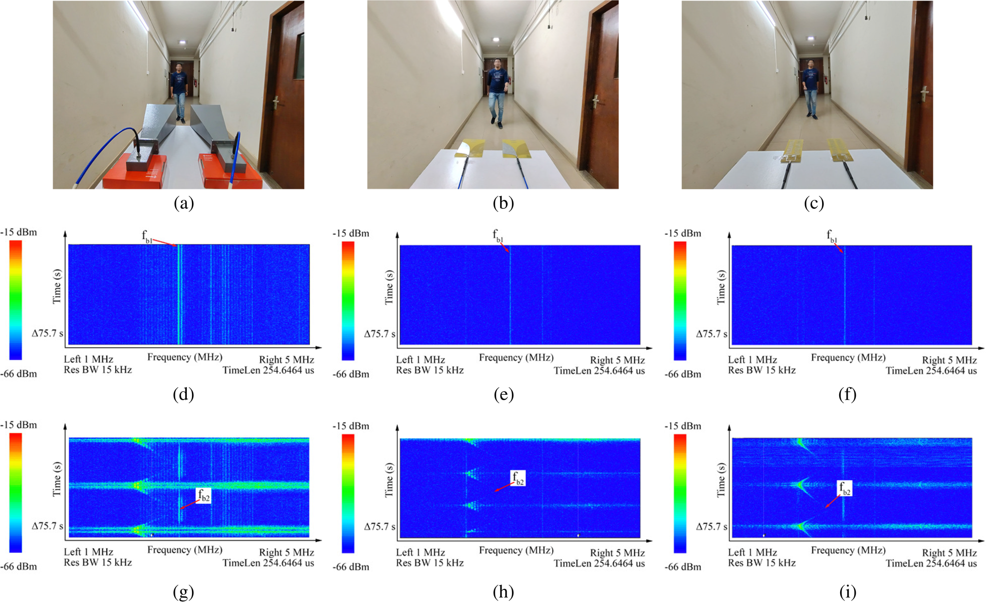
Figure 13. Snapshots showing the experimental setup (a), (b), (c), spectrograms of the static environment (d), (e), (f), and spectrograms of the walking human (g), (h), (i) in environment A for the horn, Vivaldi, and quasi-Yagi antennas, respectively.
Table 6. Environment A

Environment B
In environment B, a section of our laboratory is used. It has a wooden partition, with a sliding wooden door that acts like a low-loss wall in our experiments. The antennas are placed at a distance of 4.5 m from the back wall and the wooden partition lies at a distance of 2 m from the antennas. A volunteer walked back and forth in front of the antennas while the wooden door was kept closed.
The experimental setup, using the closed door, is shown in Figs 14(a), 14(b), and 14(c). The wooden door was closed to create a “wall-like” scenario. The volunteer then walked back and forth, behind the wooden door. First, the spectrograms for a static environment were obtained, as shown in Figs 14(d), 14(e), and 14(f). Table 7 lists the observed beat frequencies ($f_{b_{1}},\; \, f_{b_{2}},\; \, f_{b_{3}}$ ) and the corresponding distances ($d_{obs_{1}},\; \, d_{obs_{2}},\; \, d_{obs_{3}}$
 ) at which the static targets were identified by the three antennas. The closed door provides enough attenuation to make the reflections from the back wall less prominent. In the process, additional reflections due to a nearby metallic reflector are now visible. The measured distance of the wooden partition, metallic reflector, and the back wall from the antennas were d′1 = 1 m, d′2 = 2.5 m, and d′3 = 4.5 m, respectively. Next, the spectrograms for the volunteer walking behind the wooden door were obtained, as shown in Figs 14(g), 14(h), and 14(i). Table 7 lists the maximum beat frequency ($f_{b_4}$
 ) and the corresponding distance ($d_{obs_4}$
 ) up to which the signatures of the volunteer can be traced.

Figure 14. Snapshots showing the experimental setup (a), (b), (c), spectrograms of the static environment (d), (e), (f), and spectrograms of the walking human (g), (h), (i) with the door closed for the horn, Vivaldi, and quasi-Yagi antennas, respectively.
Table 7. Environment B: closed door

Through-wall measurements
For the through-wall measurements, we imaged through a 40 cm thick outer wall (brick and mortar) of our laboratory, which faces another wall on the other side of a 2 m wide corridor (Fig. 15). We used a COTS power amplifier (MAAL-010200-TR3000), which provides a power gain of 10–20 dB in the 2–2.6 GHz frequency band. The TWR setup is shown in Figs 15(a), 15(b), and 15(c). Figures 15(d), 15(e), and 15(f) show the snapshots of the spectrograms for the static environment. We can observe multiple closely spaced lines at a distance corresponding to that of the brick wall and a straight line for the outer wall of the corridor at a distance of d′ = 2 m. Table 8 lists the observed beat frequency ($f_{b_1}$ ) and the corresponding distance of the back wall ($d_{obs_1}$
 ) for all three antennas. The spectrogram signatures for the volunteer walking back and forth in front of all three antennas are shown in Figs 15(g), 15(h), and 15(i), respectively. Table 8 lists the maximum beat frequency ($f_{b_2}$
 ) and the corresponding distance ($d_{obs_2}$
 ) at which the moving target is identified. The power level of the spectrogram is kept the same for all the antennas (−25 to −125 dBm) to show the system's sensitivity. Clearly, the signatures for the case of horn antenna are more prominent than that of the Vivaldi and quasi-Yagi antennas. However, the quasi-Yagi antenna is able to identify moving targets behind the wall to distances that are quite comparable with the horn.

Figure 15. Snapshots showing the experimental setup (a), (b), (c), spectrograms of the static environment (d), (e), (f), and spectrograms of the walking human (g), (h), (i) for thru-wall measurements for the horn, Vivaldi, and quasi-Yagi antennas, respectively.
Table 8. Through-wall measurements

Using the above experiments, we have identified the range of the static objects (wall, wooden partition, metallic reflector, etc.) very close to the measured distance, as reported in Tables 6–8. Slight mismatches are due to the multiple reflections from a number of other static objects and the multi-path propagation of the waves since the experiments are conducted in a real-world situation instead of an ideal environment like an anechoic chamber. We have successfully observed the signatures of a walking human in two different environments and behind a brick wall using all three antennas. Table 9 compares the physical dimensions and weight of the three antennas used in this work. The signatures obtained from the planar antennas (Vivaldi and quasi-Yagi) may look faint when compared to the horn antenna on the same power scale but stronger signatures can be obtained by separately adjusting the mapping of the power levels for individual antennas to their respective color maps. Thus, the designed quasi-Yagi antenna can do the job as well as the horn antenna while significantly improving the portability and form factor of the complete radar system.
Table 9. Comparison of antenna size

Conclusions
This paper presents a UWB high-gain compact planar quasi-Yagi antenna with a modified ground plane for TWR application. A slot is introduced near the feed of the dipoles of the quasi-Yagi antenna in the ground plane, leading to increased effective electrical length, thereby causing miniaturization of the total antenna size. The technique offers a 22.4% reduction in dipole length and a 36% reduction in the area of a single-element antenna. The proposed antenna provides a high gain of 7.8–9.8 dBi in the entire band of interest. The antenna has a measured gain of 8.7 dBi and a front-to-back ratio of 25.76 dB at 2.4 GHz. Its size and performance are compared with planar quasi-Yagi antennas reported in recent literature and the proposed design has the maximum gain bandwidth product. The performance of the designed antennas has been characterized in an ideal anechoic chamber environment and a real-world scenario using an RoC-based system. The TWR system is then tested in different environments to study the environmental effects. The radar can successfully identify movement behind a wooden partition and a brick wall. The quasi-Yagi antenna, when compared to a horn antenna, exhibits similar levels of performance when used in a real-world system. The proposed antenna is planar, lightweight, and compact in size, compared to a bulky horn antenna and thus helps make the RoC system portable and easy to deploy.
Acknowledgments
The authors express their gratitude to Mr, Himanshu B. Sandhibigraha, Mr. Alok C. Joshi, and Mr, Rituraj Kar for their help with the experiments.
Conflict of interest
The authors declare none.
 Anand Kumar earned his B.Tech. in electronics and communication engineering (with Hons.) from the Indian Institute of Technology (ISM), Dhanbad, India, in 2020. He is presently pursuing a Ph.D. in electrical communication engineering at the Indian Institute of Science (IISc), Bengaluru, India, and was awarded the prestigious Prime Minister's Research Fellowship (PMRF) in 2022. Mr. Kumar's current research interests revolve around computational electromagnetic methods, such as finite-difference time-domain (FDTD), to model and analyze dielectrics and metamaterials with spatial and temporal dependence. He also specializes in MIMO antenna design and radar systems. Mr. Kumar has presented his research at various national and international conferences and has published his work in several peer-reviewed journals. He is dedicated to expanding our understanding of electromagnetic fields and their applications in engineering and technology, and his contributions hold great promise for the future of the field.
 Easha is a Ph.D. scholar in electrical communication engineering at the Indian Institute of Science (IISc), Bengaluru, India. She completed her B.Tech. in electronics and communication engineering from the National Institute of Technology, Patna, India, in 2020. Easha's research is focused on developing a radar-on-chip for human gait recognition and elderly fall detection, an area of great interest due to the increasing elderly population worldwide. Additionally, she is interested in phased-array antenna designs, vital signs monitoring, and through-wall imaging with radars. In recognition of her research potential, Easha was awarded the prestigious Prime Minister's Research Fellowship (PMRF) in 2022. This fellowship aims to encourage young researchers to pursue cutting-edge research and develop solutions to address challenging societal problems. Through her work, Easha seeks to develop innovative technologies that can improve the quality of life for elderly individuals and contribute to the field of radar systems.
 Dr. Debdeep Sarkar is an assistant professor in the Department of Electrical Communication Engineering (ECE), Indian Institute of Science (IISc), Bengaluru. He obtained his B.E. in ETCE from Jadavpur University, India in 2011, and his M.Tech. and Ph.D. in EE (electrical engineering) from the Indian Institute of Technology, Kanpur, in 2013 and 2018, respectively. He worked as a visiting researcher (May 2017–Aug 2017) and post-doctoral fellow (November 2018–February 2020) in the Department of Electrical and Computer Engineering, Royal Military College, Canada. He has authored one book, one book chapter, 46+ peer-reviewed journal papers, and 100+ conference papers, and he has filed three Indian patents to his credit. He regularly peer-reviews in multiple IEEE Transactions and Letters and serves as an associate editor of IET MAP and IEEE Access. He has received URSI Young Scientist Award (2019 and 2020), Infosys Young Investigator award (2020–2022), IETE Sri C. Viswanatha Reddy Memorial Award (2022), and several best paper awards.
 Dr. Gaurab Banerjee received his B.Tech. from IIT Kharagpur, Kharagpur, India, in 1997, his M.S. from Auburn University, Auburn, AL, USA, in 1999, and his Ph.D. from the University of Washington, Seattle, WA, USA, in 2006, all in electrical engineering. He has held positions at Intel Corporation (1999–2001), Intel Labs (2001–2007), and Qualcomm Inc. (2007–2010), where he worked on the design of analog and mixed-signal integrated circuits for communication systems. Since 2010, he has been a faculty member with the Department of Electrical Communication Engineering, Indian Institute of Science, Bengaluru, India. His current research interests include analog and RFICs and systems for communication and sensor applications. Dr. Banerjee has received multiple awards, including the National Talent Search Scholarship (India), Abdul Kalam Technology Innovation National Fellowship (India's highest award for translational research), and the Qualcomm Faculty Award. He was an associate editor of the IEEE Transactions on Circuits and Systems–Part I: Regular Papers from 2008 to 2010. He has served as a reviewer for many IEEE journals and conferences.


