


1. Introduction
The three-dimensional (3D) elliptical flow instability is very generic and occurs in many flow configurations, when the basic velocity field (or base flow) consists of large horizontal vortices with elliptical streamlines in their core. The elliptic instability is a parametric resonance of internal (usually inertial) waves due to an elliptical deformation of the streamlines of a rotating flow. The reader is referred to Kerswell (Reference Kerswell2002) for a detailed review and references therein. The origin of the ellipticity in the core of eddies is multifold. In the study of the stability of airplane wakes, we have to consider the presence, before their possible breaking, of a pair of large counter-rotating vortices: this is the mutual induction of these eddies that render their core elliptic. More generally, the characteristics and behaviour of counter-rotating and corotating vortex pairs have been recently reviewed in the study by Leweke, Le Dizes & Williamson (Reference Leweke, Le Dizes and Williamson2016).
In line with former studies, McKeown et al. (Reference McKeown, Ostilla-Mónico, Pumir, Brenner and Rubinstein2020) showed that iterations of the elliptical instability, arising from the interactions between counter-rotating vortices, lead to the emergence of turbulence. As a second example, in rotating flows subjected to precession, the gyroscopic torque, mediated by the misalignment of solid-body rotation and system angular velocity, induces an additional shear that, superimposed to solid-body rotation, results in elliptical streamlines, as shown by Kerswell (Reference Kerswell1993a) and by Salhi & Cambon (Reference Salhi and Cambon2009) in the simplest geometry. More generally, elliptical shape caused by tidal forces is very common in many astrophysical systems such as planetary cores, binary stars, gaseous planets and accretion discs. The importance of elliptical instability, in a purely hydrodynamic context, in the tidal dissipation mechanism in such astrophysical systems has been the subject of several studies in the literature (Barker & Lithwick Reference Barker and Lithwick2013; Cébron et al. Reference Cébron, Le Bars, Le Gal, Moutou, Leconte and Sauret2013; Barker Reference Barker2016; Barker, Braviner & Ogilvie Reference Barker, Braviner and Ogilvie2016). Note that tidal dissipation generates heat in astrophysical systems, which in some cases may be important for their structure and evolution (Ogilvie Reference Ogilvie2014).
Being the ellipticity due to the mutual induction of adjacent vortices or not, the elliptical instability is local, so that it is generally sufficient to consider a single elliptic eddy for the base (or mean) flow. For trailing vortices again, it has been shown that the Moore–Saffman–Tsai–Widnall (MSTW) instability (Moore & Saffman Reference Moore and Saffman1975; Tsai & Widnall Reference Tsai and Widnall1976), in the short-wavelength regime, is an elliptical instability (Éloy & Le Dizes Reference Éloy and Le Dizes2001; Fukumoto Reference Fukumoto2003; Sipp & Jacquin Reference Sipp and Jacquin2003; Chang & Smith Reference Chang and Smith2021). It is worth mentioning that the MSTW instability encompasses the long-wave instability bearing with Crow's instability (Crow Reference Crow1970) which occurs through the mutual induction of a pair of parallel counter-rotating vortex columns (McKeown et al. Reference McKeown, Ostilla-Mónico, Pumir, Brenner and Rubinstein2020): the Biot–Savart law is generally used to compute the induced velocity on one of the trailing vortices owing to the presence of the other. Recently, Feys & Maslowe (Reference Feys and Maslowe2016) have examined the elliptical instability of the Moore and Saffman model Moore & Saffman (Reference Moore and Saffman1975) for a single trailing vortex. Their results demonstrate the significant effect of the distribution and intensity of the axial flow on the elliptical instability of a trailing vortex. Such a robust 3D instability leads to vortex decay under most circumstances, as reviewed by Lesur & Papaloizou (Reference Lesur and Papaloizou2009). Rather old experimental evidences are quoted in the following historical review, and recently the nonlinear fate of libration-induced elliptical instability in low-dissipation and low-forcing regimes has been explored experimentally by Le Reun, Favier & Le Bars (Reference Le Reun, Favier and Le Bars2019). They showed that once the saturation of the elliptical instability is reached, a turbulent state is observed for which the energy is injected only in the resonant inertial waves.
It is clear that the elliptical instability has a very long history, and deserves a survey, as follows. This allows us to discuss what is the simplest mathematical way to identify it and to quantify its effects, first in the neutral (non-stratified), purely hydrodynamical case. After some experimental evidences of that instability (Gledzer et al. Reference Gledzer, Dolzhansky, Obukhov and Pononmarev1975; Malkus Reference Malkus1989), see also the recent review by McKeown et al. (Reference McKeown, Ostilla-Mónico, Pumir, Brenner and Rubinstein2020), a sudden interest arose when Pierrehumbert (Reference Pierrehumbert1986) discovered its characteristic properties by a conventional normal mode analysis approach, whereas at the same time Bayly (Reference Bayly1986) found the same results using the simpler and more elegant method using Kelvin modes, or mean-flow-advected (Lagrangian) Fourier modes along elliptical trajectories. The latter study, similar to that by Craik & Criminale (Reference Craik and Criminale1986), was foreshadowed by a rapid distortion theory (RDT) analysis by Cambon (Reference Cambon1982), and Cambon, Teissedre & Jeandel (Reference Cambon, Teissedre and Jeandel1985) (in French). This is re-discussed, in English, by Godeferd, Cambon & Leblanc (Reference Godeferd, Cambon and Leblanc2001), with especially its figure 3, and in Sagaut & Cambon (Reference Sagaut and Cambon2008) for a recent overview. Waleffe (Reference Waleffe1989, Reference Waleffe1990) clearly described the physical mechanism of the elliptical instability as a vortex stretching mechanism and showed how the growing Kelvin modes found by Bayly (Reference Bayly1986) in the case of unbounded strained vortex could be superimposed to create a localised, unstable disturbance of the form found in the bounded elliptical cylinder case (Gledzer et al. Reference Gledzer, Dolzhansky, Obukhov and Pononmarev1975).
From the previous studies, let us summarise the advantages of the formalism with projection of the disturbance fields onto Kelvin modes. The Kelvin modes are essentially 3D Fourier modes, even if the wave vector can become time-dependent following the mean flow streamlines. The time dependency of the wave vector represents the convection of the plane wave  $\exp (\mathrm {i} \boldsymbol {k}(t)\boldsymbol {\cdot }\boldsymbol {x})$ by the base flow. Both the direction and magnitude of $\boldsymbol {k}$ change as wave crests rotate and approach or separate from each other due to basic velocity gradients. Accordingly, all the formal advantages of Fourier space remain valid: pure algebraic formulation of integro-differential equations, including Poisson equation for pressure disturbances, algebraic dissipation term instead of Laplacian operator, algebraic linkage from vorticity to velocity (instead of a Biot–Savart relationship). It is worth emphasising that the system of equations for disturbances in terms of Lagrangian Fourier modes is universal under a typical length scale. Indeed, such a system is recovered for small-scale disturbances traveling near any smooth base-flow trajectory, in the zonal asymptotic method of Lifschitz & Hameiri (Reference Lifschitz and Hameiri1991) with close connection with geometric optics; the velocity gradients of the base flow are treated as space-uniform in a domain of unspecified length scale, asymptotically small (see also Godeferd et al. Reference Godeferd, Cambon and Leblanc2001).
Can the elliptic instability, in the pure hydrodynamic context, survive in the presence of vertical basic density stratification, that is stabilising considered alone? A first answer is given by the study of the stability of inertia-gravity waves when it is altered by the ellipticity of streamlines. In relation to the dynamics of ocean and atmosphere (Miyazaki & Fukumoto Reference Miyazaki and Fukumoto1992; Miyazaki Reference Miyazaki1993) investigated the influence of the Coriolis force and density stratification, caused by temperature or salinity gradient, on the elliptical instability. Miyazaki & Fukumoto (Reference Miyazaki and Fukumoto1992) considered an unbounded strained-vortex flow with stable axial stratification. They have found that the growth rates for the elliptical instability were invariably reduced: the subharmonic elliptical instability is completely suppressed when Brunt–Väisälä frequency ( $N)$ is greater or equal to the half of the basic vorticity strength ( $\varOmega ).$ For small eccentricities, asymptotic theory leads to formulae for the maximum growth rate (Kerswell Reference Kerswell2002) (see also § 3 in the present study). It is worth mentioning that the elliptical instability of stratified vortices has been addressed as well in previous studies (Otheguy, Chomaz & Billant Reference Otheguy, Chomaz and Billant2006; Le Bars & Le Dizès Reference Le Bars and Le Dizès2006; Guimbard et al. Reference Guimbard, Le Dizès, Le Bars, Le Gal and Leblanc2010; Suzuki, Hirota & Hattori Reference Suzuki, Hirota and Hattori2018). The effects of differential diffusion between momentum and density on the elliptical instability have recently been addressed by Singh & Mathur (Reference Singh and Mathur2019). They showed that, in the case where the ratio of thermal diffusivity to kinematic diffusivity is equal to unity, the viscous effects are purely suppressive, whereas for sufficiently small values of this ratio, there is an oscillatory instability whose signature is nevertheless present with zero growth rate in the inviscid limit. In turbulent Rayleigh–Bénard convection, Zwirner, Tilgner & Shishkina (Reference Zwirner, Tilgner and Shishkina2020) showed that the mechanism which causes the twisting and breaking of a single-roll large-scale circulation into multiple rolls is the elliptical instability. On the other hand, density effects on the MSTW instability have been recently investigated by Chang & Smith (Reference Chang and Smith2021) who performed a normal mode stability analysis and showed that, for the subharmonic instability (resonance $(m,m+2)=(0,2),$ $m$ being the azimuthal wavenumber) the growth rate is maximised when the ratio of vortex to ambient fluid density is near $0.215$.
The interaction of vortices with a magnetic field is a fundamental process in astrophysical magnetohydrodynamics (MHD). Therefore, a similar question occurs when one moves from hydrodynamics to MHD when the electrically conducting elliptical flow is subjected to an unperturbed (or a basic) magnetic field. In a geophysical context, Kerswell (Reference Kerswell1994) studied the effect of a toroidal magnetic field on the elliptic instability in a rotating spheroidal container filled with an incompressible electrically conducting fluid, which carries a constant axial electric current. He concluded that the toroidal magnetic field has a stabilising influence. By including the effect of a uniform magnetic field perpendicular to the plane of the elliptical base flow, the resulting magneto-elliptic instability has been related to the problem of turbulence generation and, hence, momentum transport in accretion discs by Lebovitz & Zweibel (Reference Lebovitz and Zweibel2004) (hereafter LZ04). In that study, an analytical technique was developed to determine the maximal growth rates of the destabilising resonances of order  $n=2$ (i.e. subharmonic instabilities, see (1.1)) in the limit of small elliptical (tidal) deformations. This analytical technique has been used in previous studies by Mizerski & Bajer (Reference Mizerski and Bajer2009) for the magneto-elliptical instability of rotating systems and by Salhi, Lehner & Cambon (Reference Salhi, Lehner and Cambon2010) for the magneto-precessional instability. Herreman et al. (Reference Herreman, Cébron, Le Dizès and Le Gal2010) conducted experiments to explain some aspects of the nonlinear transition process for the elliptic instability in rotating cylinders under imposed magnetic field. It is worth noting that in the case where the Coriolis and Lorentz forces are simultaneously present and when the wave vector $\boldsymbol {k}$ aligns with the magnetic field the elliptical flow can develop horizontal instability which dominates over all other modes (Bajer & Mizerski Reference Bajer and Mizerski2013). In the astrophysical context (tidal dissipation in gaseous planets and stars), Barker & Lithwick (Reference Barker and Lithwick2014) found that magnetic fields do prevent vortices from forming and, hence, greatly enhance the steady-state dissipation rate.
The combined effects of stable density stratification and MHD on the elliptical instability within an elliptically distorted cylinder have been investigated by Kerswell (Reference Kerswell1993b). He performed a normal mode stability analysis for a simple configuration possessing considerable symmetry between the velocity and magnetic fields: a purely azimuthal magnetic field, which in the frozen flux limit is also elliptically distorted. In that study, stratification is either axial (the isopycnics are parallel to the streamlines) or radial (the isopycnics are perpendicular to the streamlines).
In the present paper we analyse in detail the joint influence of a stable axial stratification (with strength  $N)$ and an external (axial) uniform magnetic field (with Alfvén velocity scaled from the basic magnetic field $B)$ on the stability of an unbounded flow with elliptical streamlines of a perfectly conducting fluid. Our study extends the study by Miyazaki & Fukumoto (Reference Miyazaki and Fukumoto1992) by including the effects of a magnetic field and also the study by LZ04 by including the effects of an axial stable stratification. An important aspect of the present study is to map out the regime of $(B/(L_0\varOmega ), N/\varOmega )$ space ( $L_0$ being a characteristic length scale) for which the destabilising resonances of order $n=2$ (see (1.1)) of magneto-inertia-gravity (MIG) waves prone to operate and to determine their growth rates at small ellipticity by extending the analytical technique by LZ04. In the laboratory experiment of a magnetised turbulent Taylor–Couette flow of liquid metal by Nornberg et al. (Reference Nornberg, Ji, Schartman, Roach and Goodman2010), the combined fast and slow Alfvén-inertial waves were clearly identified where the observed slow wave is damped. These authors have identified a relationship between the slow magneto-inertial waves and the magneto-rotational instability (MRI) (Balbus & Hawley Reference Balbus and Hawley1991; Wang et al. Reference Wang, Gilson, Ebrahimi, Goodman and Ji2022). On the other hand, Mizerski & Lyra (Reference Mizerski and Lyra2012) examined the link between the magneto-elliptical instability and the MRI, explaining that the two instabilities are different manifestations of the same magneto-elliptical-rotational instability. Salhi et al. (Reference Salhi, Lehner, Godeferd and Cambon2012) have studied the effects of stable stratification on the MRI instability and showed that, under the MHD Boussinesq approximation (e.g. Wilczyński, Hughes & Kersalé Reference Wilczyński, Hughes and Kersalé2022), the so-called ‘magnetic induction potential scalar’ (MIPS, i.e. the scalar product of the magnetic field vector and the density gradient) is a Lagrangian invariant for a non-diffusive fluid. In contrast, the potential vorticity (PV), which is very useful as an invariant in stratified geophysical flows (e.g. Pedlosky Reference Pedlosky2013), is no longer valid in MHD because it removes the baroclinic torque in the extended vorticity equation, but not the counterpart of the Lorentz force.
An asymptotic stability analysis is developed in § 3 at leading order in the ellipticity parameter  $\varepsilon$ in order to determine the growth rates of the (subharmonic) instability tongues that emanate from the points at vanishing ellipticity. In this limit, disturbances to the basic flow are found in terms of MIG dispersive waves, with a dispersion law (Salhi et al. Reference Salhi, Baklouti, Godeferd, Lehner and Cambon2017) that includes $\varOmega,$ $N,$
$N,$  $B/L_0$ and the angular parameter $\mu =\cos (\theta )$ (the angle $\theta$ being the angle between the wave vector of the perturbations and that of the base-flow vorticity). In contrast with particular cases, the general dispersion law of MIG waves is no longer a simple combination of the individual dispersion frequencies, considered alone, but is obtained in combining the eigenvalues of the matrix of the whole linear system of equations (Salhi et al. Reference Salhi, Baklouti, Godeferd, Lehner and Cambon2017). Fast and slow modes are identified, with different resonance conditions between them, or
 \begin{equation} \omega_i-\omega_j=n\varOmega\quad (i,j=1,2,3,4,\ i\ne j,\ n \ \text{being an integer}). \end{equation}
Without an analysis of the resonant conditions, it is not possible to simply identify the different instabilities, namely if they are subharmonic or not, if they result from the interaction of two fast modes, two slow modes, or one fast and one slow.
As detailed in § 2, the use of the magnetic invariant (MIPS) makes it possible to reduce the linear system of ordinary differential equations, which represents a Floquet problem, from a five-component system to a four-component system only. In § 3, we show that stable stratification enhances the destabilising resonance of order  $n=2$ between two slow modes because we find that, at large magnetic strengths, its growth rate is about twice that found in the case without stratification (LZ04). Asymptotic formulae are compared with numerical results carried out at arbitrary ellipticity in § 4. The effect of diffusion is briefly addressed in the special case where the diffusion coefficients (kinetic, thermal and magnetic) are equal. Conclusions and perspectives are offered in § 5.
2. MHD Boussinesq's equations
We consider a stratified electrically conducting fluid. Density variations are introduced using the Boussinesq approximation for simplicity (Chandrasekhar Reference Chandrasekhar1961). The fluid is assumed to be inviscid and non-diffusive. The effect of viscosity ( ${\nu })$ and thermal ( $\kappa )$ and magnetic ( $\eta )$ diffusivity are briefly addressed in § 4.3 by considering the case where $\nu =\kappa =\eta$ (i.e. the case where the magnetic and thermal Prandtl numbers are unity).
The Boussinesq MHD equations written in a fixed frame take the form (Davidson Reference Davidson2013)
 $$\begin{gather} D_t{\tilde{\boldsymbol{u}}}=-{\boldsymbol{\nabla}} \tilde{p}+\left (\tilde{\boldsymbol{b}} \boldsymbol{\cdot} \boldsymbol{\nabla}\right)\tilde{\boldsymbol{b}} +\tilde{\vartheta}\boldsymbol{n}+{\nu} \nabla^2 \tilde{\boldsymbol{u}}, \end{gather}$$
 $$\begin{gather}D_t{\tilde{\boldsymbol{b}}}= \left (\tilde{\boldsymbol{b}}\boldsymbol{\cdot}\boldsymbol{\nabla}\right) \tilde{\boldsymbol{u}}+\eta\nabla^2\tilde{\boldsymbol{b}}, \end{gather}$$
 $$\begin{gather}D_t{\tilde{\vartheta}}=\kappa\nabla^2\tilde{\vartheta}, \end{gather}$$
 $$\begin{gather}\boldsymbol{\nabla}\boldsymbol{\cdot} {\tilde{\boldsymbol{u}}}=0, \end{gather}$$
 $$\begin{gather}\boldsymbol{\nabla}\boldsymbol{\cdot} {\tilde{\boldsymbol{b}}}=0, \end{gather}$$
where  $D_t(\boldsymbol {\cdot })\equiv (\partial _t +\tilde {\boldsymbol {u}}\boldsymbol {\cdot }\boldsymbol {\nabla })(\boldsymbol {\cdot })$ denotes the material derivative, $\tilde {\boldsymbol {u}}$ denotes the velocity and $\tilde {\boldsymbol {b}}$ denotes the magnetic field which is scaled using Alfvén velocity units, i.e. it is divided by $\sqrt {\rho _0\mu _0}$ where $\rho _0$ and $\mu _0$ are the constant density and the magnetic permeability of the fluid. Here, $\tilde {p}$ being the total pressure (including the magnetic part) divided by the constant density $\rho _0.$ In the present study, we consider axial stratification,
 \begin{equation} \boldsymbol{n}=\boldsymbol{e}_3=-\boldsymbol{g}/g. \end{equation}
where  $\boldsymbol {e}_3$ is the upward vertical unit vector and $\boldsymbol {g}$ is the gravitational acceleration vector. The first equation in the above system is the momentum equation, the second is the induction equation for the magnetic field and the third is the buoyancy scalar equation. Both velocity field and magnetic field are solenoidal (2.1d,e).
For a non-magnetised Boussinesq ideal fluid, one may easily show that the PV (Pedlosky Reference Pedlosky2013),
 \begin{equation} {\tilde{\varpi}_\kappa=\tilde{\boldsymbol{\omega}}_a\boldsymbol{\cdot}\boldsymbol{\nabla} \tilde{\vartheta}} ,\end{equation}
 is a Lagrangian, invariant, i.e.  $D_t\tilde {\varpi }_\kappa =0.$ Here, $\tilde {\boldsymbol {\omega }}_a$ is the absolute vorticity vector which, in the absence of the Coriolis force, identifies with the vorticity vector $\boldsymbol {W}=\boldsymbol {\nabla } \times \tilde {\boldsymbol {u}}.$ A counterpart, for a magnetised Boussinesq ideal fluid, is the so-called MIPS (Salhi et al. Reference Salhi, Lehner, Godeferd and Cambon2012)
 \begin{equation} \tilde{\varpi}_m=\tilde{\boldsymbol{b}}\boldsymbol{\cdot}\boldsymbol{\nabla} \tilde{\vartheta} \end{equation}
that is a Lagrangian invariant, i.e.  $D_t\tilde {\varpi }_m=0,$ and not $\tilde {\varpi }_\kappa.$ The usefulness of introducing the MIPS is illustrated later.
2.1. Base flow
The solutions of system (2.1) are conveniently decomposed into a ‘basic flow’  $(\boldsymbol {U},P, \boldsymbol {B}, \varTheta )$ and a ‘disturbance’ $(\boldsymbol {u},p,\boldsymbol {b}, \vartheta ),$ but the latter needs to be small compared with the former,
 \begin{equation} \tilde{\boldsymbol{u}}=\boldsymbol{U}+\boldsymbol{u},\quad \tilde{p}=P+p,\quad \tilde{\boldsymbol{b}}=\boldsymbol{B}+\boldsymbol{b},\quad {\tilde{\vartheta}}=\varTheta+\vartheta. \end{equation}
We consider the linear stability of a stratified vortical flow with elliptical streamlines and with uniform vertical magnetic field (see figure 1)
 $$\begin{gather} \boldsymbol{U}={\boldsymbol{A}}\boldsymbol{\cdot} \boldsymbol{x},\quad {\boldsymbol{A}}=\varOmega \left (\begin{array}{@{}ccc@{}} 0 & -E & 0\\ E^{-1} & 0 & 0\\ 0 & 0 & 0 \end{array}\right) \end{gather}$$
 $$\begin{gather}\boldsymbol{B}=B\boldsymbol{e}_3, \end{gather}$$
 $$\begin{gather}\varTheta=N^2x_3 \end{gather}$$
where  $\varOmega$ is a constant that is a measure of the intensity of the flow and $E\geq 1$ is a measure of elliptical deformation of the streamlines, and $N$ is the Brunt–Väisälä frequency such that
 \begin{equation} N^2=-\frac{g}{\rho_0}\frac{{\rm d}\varrho}{{\rm d}\kern 0.06em x_3}. \end{equation}
Circular streamlines correspond to the case where  $E=1.$ The parameter
 \begin{equation} \varepsilon=\tfrac{1}{2}\left (E-E^{-1}\right) \end{equation}
represents the departure of the streamlines of the unperturbed flow from axial symmetry. We note that
 \begin{equation} 0<\delta=(E-E^{-1})/(E+E^{-1})<1 \end{equation}
for the flow to be elliptical. We also note that, an equivalent form for the unperturbed velocity field has been used in previous studies (Waleffe Reference Waleffe1990; Miyazaki & Fukumoto Reference Miyazaki and Fukumoto1992; Miyazaki Reference Miyazaki1993; Kerswell Reference Kerswell2002; Mizerski & Bajer Reference Mizerski and Bajer2009; Bajer & Mizerski Reference Bajer and Mizerski2013)
 \begin{equation} \boldsymbol{U}={\varGamma}\left [-\left (1+\delta\right)x_2\boldsymbol{e}_1+\left (1-\delta\right)x_1\boldsymbol{e}_2\right], \end{equation}
where  $2{\varGamma }={\varOmega } (E+E^{-1} )$ and $-{\varGamma }\delta$ represents the strain rate, but the expression (2.6a) seems more suitable for analysing resonant destabilisation (Mizerski & Bajer Reference Mizerski and Bajer2009).

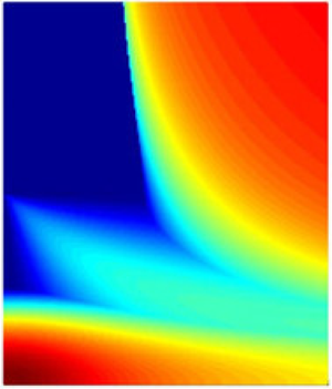
Figure 1. A schematic drawing of the basic state: planar flow with elliptical streamlines,  $\varPsi =-(\varOmega /2) (E^{-1}x_1^2+Ex_2^2)$ being the stream function in the presence of an axial uniform magnetic field ( $\boldsymbol {B}=B\boldsymbol {e}_3)$ and an axial stable stratification ( $\varTheta =N^2x_3,$ $N^2=-(g/\rho _0)({\rm d}\varrho /{\rm d}\kern 0.06em x_3)$, $N$ being the Brunt–Väisälä frequency). The gravity vector is given by $\boldsymbol {g}=-g\boldsymbol {e}_3$ with $g > 0$.
The basic buoyancy scalar  $\varTheta$ varies linearly with the axial coordinate $x_3$ (axial stratification) and is proportional to the gravitational acceleration, $g,$ and to a background density (or temperature) gradient. This linear profile admits a constant Brunt–Väisälä frequency $N$ throughout the entire fluid. More general exact solutions of the combined stratified fluid/magnetic equations exist in an unbounded domain (Craik Reference Craik1989); the case in hand (i.e. (2.6)) is probably the simplest of these. As indicated previously, Miyazaki & Fukumoto (Reference Miyazaki and Fukumoto1992) considered an unbounded strained-vortex flow with stable exponential stratification in the axial direction at small Froude number, ${Fr}={\varGamma }^2L_0/g\ll 1$ with $L_0$ a characteristic length scale. One may show that the resulting linear differential system for the disturbances superimposed on the base flow is the same considering either an exponential basic stratification or a linear (with respect to space coordinates) basic stratification. Both profiles (exponential or linear) admit a constant Brunt–Väisälä frequency throughout the entire fluid.
2.2. Perturbed system
In the following, we consider the case of a non-diffusive fluid. Diffusivity effects with the assumption that the diffusion coefficients are equal  $({\nu }=\kappa =\eta )$ or, equivalently, the magnetic and thermal Prandtl numbers are equal to one are briefly discussed at the end of § 4.
2.2.1. Linearised system in physical space
We substitute the solutions (2.5a–d) into the system (2.1) and linearise. Linearisation is not readily justified by the fact that the flow disturbances are very small with respect to the base flow. Linearisation is briefly discussed in the conclusion. Thus, we expect our analysis to break down when the disturbances become so large that nonlinear effects become important. The resulting perturbed equations are
 $$\begin{gather} D_t{\boldsymbol{u}}=-\boldsymbol{\nabla} p-\left (\boldsymbol{u}\boldsymbol{\cdot}\boldsymbol{\nabla}\right)\boldsymbol{U}+ \left ({\boldsymbol{B}}\boldsymbol{\cdot}\boldsymbol{\nabla}\right)\boldsymbol{b}+ \vartheta\boldsymbol{e}_3, \end{gather}$$
 $$\begin{gather}D_t{\boldsymbol{b}}= \left ({\boldsymbol{b}}\boldsymbol{\cdot}\boldsymbol{\nabla}\right){\boldsymbol{U}}+\left ({\boldsymbol{B}}\boldsymbol{\cdot}\boldsymbol{\nabla}\right){\boldsymbol{u}}, \end{gather}$$
 $$\begin{gather}D_t{\vartheta}=-N^2u_3, \end{gather}$$
 $$\begin{gather}\boldsymbol{\nabla}\boldsymbol{\cdot} {\boldsymbol{u}}=0, \end{gather}$$
 $$\begin{gather}\boldsymbol{\nabla}\boldsymbol{\cdot} {\boldsymbol{b}}=0. \end{gather}$$
As for the linear part of MIPS (see (2.4)), it takes the form
 \begin{equation} \varpi_m=B\frac{\partial \vartheta}{\partial x_3}+ N^2b_3, \end{equation}
where  $D_t\varpi _m=0,$ so that $\varpi _m=\text {const}.$ As shown later, for the purposes of studying stability, we may set $\varpi _m=0$ (see also Benkacem et al. Reference Benkacem, Salhi, Khlifi, Nasraoui and Cambon2022).
2.2.2. Floquet system in wave space
The disturbances are expressed in terms of Lagrangian Fourier modes, as discussed in section 1. These modes were used for shear waves by Moffatt (Reference Moffatt2010), who was probably the first to call them ‘Kelvin modes’, in reference to a pioneering paper by Lord Kelvin Kelvin (Reference Kelvin1887) in the nineteenth century. They are advected by the mean flow as Lagrangian invariants (Cambon Reference Cambon1982; Sagaut & Cambon Reference Sagaut and Cambon2008), as plane waves for which the direction and the speed of propagation depend on time, via a time-dependent wave vector:
 \begin{equation} \left [\boldsymbol{u},p,\boldsymbol{b},\vartheta\right](\boldsymbol{x},t)= \left [\hat{\boldsymbol{u}},\hat{p}, \hat{\boldsymbol{b}}, \hat{\vartheta}\right] (\boldsymbol{k},t)\exp\left ({\mathrm{i}}\boldsymbol{x}\boldsymbol{\cdot}\boldsymbol{k}(t)\right), \end{equation}
where  $\mathrm {i}^2=-1.$ Accordingly, the material derivative of the fluctuating velocity can be rewritten as
 \begin{equation} D_t{{\boldsymbol{u}}}=\left (\partial_t+U_j\frac{\partial }{\partial x_j}\right)\left [\hat{\boldsymbol{u}}(\boldsymbol{k},t)\exp\left ({\mathrm{i}}\boldsymbol{x}\boldsymbol{\cdot}\boldsymbol{k}(t)\right)\right] \end{equation}
with  $U_j=A_{jm}x_m,$ so that
 \begin{equation} D_t{{\boldsymbol{u}}}=\left [\partial_t{\hat{\boldsymbol{u}}}+\mathrm{i} \left ((d_t k_j)x_j+A_{jm}k_jx_m\right)\hat{\boldsymbol{u}}\right ] \exp\left ({\mathrm{i}}\boldsymbol{x}\boldsymbol{\cdot}\boldsymbol{k}(t)\right), \end{equation}
or, equivalently,
 \begin{equation} D_t{{\boldsymbol{u}}}=\left (\partial_t{\hat{\boldsymbol{u}}}+\mathrm{i} \left [\left (d_t \boldsymbol{k}+A^T\boldsymbol{k}\right)\boldsymbol{\cdot}\boldsymbol{x}\right]\hat{\boldsymbol{u}}\right ) \exp\left ({\mathrm{i}}\boldsymbol{x}\boldsymbol{\cdot}\boldsymbol{k}(t)\right). \end{equation}
In order to remove the explicit dependence on  $\boldsymbol {x}$ in the resulting equations for the Fourier amplitudes $\hat {\boldsymbol {u}},$ $\hat {\boldsymbol {b}},$ $\hat {p}$ and $\hat {\vartheta },$ one has to ensure that $\boldsymbol {k}(t)$ varies in time according to the eikonal equation
 \begin{equation} {d_t{\boldsymbol{k}}}=-{\boldsymbol{A}}^T\boldsymbol{\cdot}\boldsymbol{k}, \end{equation}
where  $d_t(\boldsymbol {\cdot })\equiv {{\rm d}(\boldsymbol {\cdot })}/{{\rm d}t}$ and $T$ denotes transpose. Equation (2.17) can be solved to give
 \begin{equation} k_1=k_{p}\cos(\tau-\phi),\quad k_2=Ek_{p}\sin (\tau -\phi),\quad k_3=k_{30}, \end{equation}
where  $\tau =\varOmega t$ being a dimensionless time,
 \begin{equation} k_p^2=k_1^2+E^{-2}k_2^2=k_{10}^2+E^{-2}k ^2_{20},\quad \tan \phi=-E^{-1}k_{20}/k_{10}, \end{equation}
with  $k_{j0}$ ( $\,j=1,2,3)$ the initial wave vector component. For purposes of studying stability, we may set $\phi =0$. This is easily seen by making the substitution $\varOmega t'=\varOmega t+\phi,$ which eliminates $\phi$ from the equation.
Substituting the plane waves solution (2.13) into the system (2.11) and taking into account the eikonal equation (2.17), we obtain
 $$\begin{gather} d_t{\hat{\boldsymbol{u}}}=-\mathrm{i} \hat{p}\boldsymbol{k}-{\boldsymbol{A}}\boldsymbol{\cdot} {\hat{\boldsymbol{u}}}+\mathrm{i} \left (k_3B\right)\hat{\boldsymbol{b}}+ \hat{\vartheta}\boldsymbol{e}_3, \end{gather}$$
 $$\begin{gather}d_t{\hat{\boldsymbol{b}}}={\boldsymbol{A}}\boldsymbol{\cdot}\hat{\boldsymbol{b}}+\mathrm{i} \left (k_3B\right)\hat{\boldsymbol{u}}, \end{gather}$$
 $$\begin{gather}d_t{\hat{\vartheta}}=-N^2\hat u_3, \end{gather}$$
together with  $\boldsymbol {k}\boldsymbol {\cdot }\hat {{\boldsymbol {u}}}=0$ and $\boldsymbol {k}\boldsymbol {\cdot } \hat {{\boldsymbol {b}}}=0.$ The use of the latter conditions allows one to eliminate the Fourier amplitude of fluctuating pressure,
 \begin{equation} \hat p(\boldsymbol{k},t)=-\mathrm{i} k^{-2}\left (2\varOmega^2\hat{c}_1+k_3\hat{\vartheta}\right),\quad \varOmega\hat{c}_1= Ek_1\hat u_2-E^{-1}k_2\hat u_1, \end{equation}
and to reduce the above seven-component Floquet system to a five-component version. Here,  $k = \sqrt {k_1^2+k_2^2 + k_3^2}$ is the modulus of the wave vector. This reduction of components results from the fact that both Fourier modes for fluctuating velocity and for fluctuating magnetic field are two-component in the plane normal to the wave vector. Such projection can be done using the orthonormal Craya–Herring frame of reference, as used in several articles (e.g.from Salhi & Cambon Reference Salhi and Cambon1997).
We note that the case where the wave vector is vertical, so that  $k_1 = k_2 = 0,$ $k_p = 0$ and $k_3 = \pm k,$ characterises a special class of disturbances, called horizontal perturbations, in which the vertical components $\hat {u}_3$ and $\hat {b}_3$ identically vanish (Bajer & Mizerski Reference Bajer and Mizerski2013). In that case, axial stratification has no effect on the horizontal perturbations, and then there is no instability without the Coriolis force.
2.2.3. Change of variables
At  $k_3=0,$ the solution of the resulting Floquet system (2.20) is stable. Accordingly, we henceforth consider only perturbations with vertical wave number $k_3\ne 0.$ As in the studies by LZ04 and by Mizerski & Bajer (Reference Mizerski and Bajer2009), we transform the resulting Floquet system in terms of the following variables to facilitate subsequent calculations
 \begin{align} \varOmega\hat{c}_2=-k_3\hat{u}_3,\quad \varOmega\hat{c}_3=Ek_1\hat{b}_2-E^{-1}k_2\hat{b}_1,\quad \varOmega \hat{c}_4=-k_3\hat{b}_3,\quad \varOmega^2\hat{c}_5=-k_3\hat{\vartheta}. \end{align}
Given (2.21a,b) we transform the system (2.20) according to these new variables,
 $$\begin{gather} d_\tau{\hat{c}}_1=-4\varepsilon \frac{k_1k_2}{k^2}\hat{c}_1-2\hat{c}_2+\mathrm{i} \frac{(k_3B)}{\varOmega}\hat{c}_3+2\varepsilon \frac{k_1k_2}{k^2}\hat{c}_5, \end{gather}$$
 $$\begin{gather}d_\tau{\hat{c}}_2=2\frac{k_3^2}{k^2}\hat{c}_1+\mathrm{i} \frac{(k_3B)}{\varOmega} \hat{c}_4+\frac{k_\perp^2}{k^2}\hat{c}_5, \end{gather}$$
 $$\begin{gather}d_\tau{\hat{c}}_3=\mathrm{i} \frac{(k_3B)}{\varOmega}\hat{c}_1, \end{gather}$$
 $$\begin{gather}d_\tau{\hat{c}}_4=\mathrm{i} \frac{(k_3B)}{\varOmega}\hat{c}_2, \end{gather}$$
 $$\begin{gather}d_\tau{\hat{c}}_5=-\frac{N^2}{\varOmega^2}\hat{c}_2, \end{gather}$$
where  $d_\tau {\hat {c}}_1= \varOmega ^{-1}d_t\hat {c}_1$ and $k_\perp =\sqrt {k_1^2+k_2^2}.$ Combining (2.23d) and (2.23e), we deduce the following relation:
 \begin{equation} -\frac{\varOmega}{k_3}\left [\mathrm{i}\varOmega\left (k_3B\right)\hat{c}_5+N^2\hat{c}_4\right]=\mathrm{i}\left (k_3B\right)\hat{\vartheta}+N^2\hat{b}_3=\hat{\varpi}_m=\text{const.}, \end{equation}
which represents the spectral counterpart of the MIPS (see (2.4)). Accordingly, system (2.23) can be further reduced to a fourth-order inhomogeneous Floquet system,
 \begin{equation} d_\tau{\hat{\boldsymbol{c}}}={\boldsymbol{D}}(\tau)\boldsymbol{\cdot}{\hat{\boldsymbol{c}}}+\hat{\boldsymbol{\varphi}}, \end{equation}
where the only non-zero elements of  ${\boldsymbol {D}}(\tau )$ are
 $$\begin{gather} D_{11}=-4\varepsilon \frac{k_1k_2}{k^2},\quad D_{12}=-2,\quad D_{21}=2\frac{k_3^2}{k^2}, \end{gather}$$
 $$\begin{gather}D_{13}=D_{31}=D_{42}=\mathrm{i} \frac{\left (k_3B\right)}{\varOmega}, \end{gather}$$
 $$\begin{gather}D_{14}=2\mathrm{i} \varepsilon \frac{N^2}{\varOmega (k_3B)}\frac{k_1k_2}{k^2}, \end{gather}$$
 $$\begin{gather}D_{24}=\mathrm{i} \left (\frac{\left (k_3B\right)}{\varOmega}+ \frac{N^2}{\varOmega \left (k_3B\right)}\frac{k_\perp^2}{k^2}\right). \end{gather}$$
The non-zero components of the inhomogeneous term in (2.25) take the form
 $$\begin{gather} \hat{\varphi}_{1}=2\mathrm{i} \varepsilon\frac{k_1k_2}{k^2}\frac{\hat{\varpi}_m}{(\varOmega^2 B)}, \end{gather}$$
 $$\begin{gather}\hat{\varphi}_{2}=\mathrm{i} \frac{k_\perp^2}{k^2} \frac{\hat{\varpi}_m}{(\varOmega^2 B)} \end{gather}$$
and it can be seen as a time-varying forcing excitation.
Note that in the non-magnetised stratified case, one can use the fact that the PV is a Lagrangian invariant for a non-diffusive fluid (Pedlosky Reference Pedlosky2013) to derive a non-homogeneous two-component Floquet system in terms of the variables  $\hat {c}_1$ and $\hat {c}_2.$
2.3. Homogeneous Floquet system
The linear system (2.25) has the properties  ${\boldsymbol {D}}(\tau +T)= {\boldsymbol {D}}(\tau )$ and $\hat {\boldsymbol {\varphi }}(\tau +T)= \hat {\boldsymbol {\varphi }}(\tau )$ where $T=2{\rm \pi}$ is the period common to both the matrix ${\boldsymbol {D}}$ and the vector $\hat {\boldsymbol {\varphi }}$. Floquet theory does not address stability of the inhomogeneous system described by (2.25) where the ‘forcing excitation’ $\hat {\boldsymbol {\varphi }}(\tau )$ is present. However, the $T$-periodic nature of $\hat {\boldsymbol {\varphi }}(\tau )$ allows an extension to the theory (Slane & Tragesser Reference Slane and Tragesser2011). Following the study of Slane & Tragesser (Reference Slane and Tragesser2011), it is shown that the basic behaviour of the homogeneous system
 \begin{equation} d_\tau\hat{\boldsymbol{c}}={\boldsymbol{D}}\boldsymbol{\cdot}\hat{\boldsymbol{c}} \end{equation}
does not change with the addition of the term  $\hat {\boldsymbol {\varphi }}(\tau ).$ Here, $\hat {\boldsymbol {c}}=(\hat {c}_1,\hat {c}_2,\hat {c}_3,\hat {c}_4)^{\rm T}$ in the canonical basis of $\mathbb {C}^4.$ In other words, for purposes of studying stability, one may set $\hat {\varpi }_\kappa =0,$ so that $\hat {\boldsymbol {\varphi }}=\boldsymbol {0}$ (Benkacem et al. Reference Benkacem, Salhi, Khlifi, Nasraoui and Cambon2022).
We denote by  $\boldsymbol {\varPhi }(\tau )$ any fundamental matrix solution of the homogeneous system (2.28) where $\boldsymbol {\varPhi }(0)={\boldsymbol {I}}_4$. According to Floquet–Lyapunov theorem, $\boldsymbol {\varPhi }$ is expressible in the form (Kuchment Reference Kuchment1993),
 \begin{equation} \boldsymbol{\varPhi}(\tau)={\boldsymbol{F}}(\tau)\exp\left ({\boldsymbol{K}}\tau\right), \end{equation}
where  ${\boldsymbol {F}}(\tau )$ is a non-singular continuous $2{\rm \pi}$-periodic $4\times 4$ matrix-function (whose derivative is an integrable piecewise-continuous function) and ${\boldsymbol {K}}$ is a constant matrix. The determinant of $\boldsymbol {\varPhi }$ is unity at $\tau =2{\rm \pi},$ $\vert {\boldsymbol {\varPhi } (2{\rm \pi} )}\vert =1$ because
 \begin{equation} \text{trace}\,{\boldsymbol{D}}=\sum_{j=1}^4D_{jj}=-4\varepsilon \frac{k_1k_2}{k^2}=-\frac{1}{k^2}{d_\tau k^2}. \end{equation}
It follows that whenever  $\lambda$ is an eigenvalue of the monodromy matrix, ${\boldsymbol {M}}=\boldsymbol {\varPhi }(2{\rm \pi} ),$ so too are its inverse $\lambda ^{-1}$ and its complex conjugate $\lambda ^*$ (see LZ04). Consequently, in the stable case, eigenvalues of ${\boldsymbol {M}}$ lie on the unit circle. If any eigenvalue $\lambda$ of ${\boldsymbol {M}}$ has modulus exceeding one, this implies that there is indeed an exponentially growing solution. The growth rates are then given by
 \begin{equation} \sigma=\frac{1}{2{\rm \pi}}\log \left (\lambda\right). \end{equation}
In the Floquet system (2.28) figure four dimensionless parameters, namely
 \begin{equation} \varepsilon=\tfrac{1}{2}\left (E-E^{-1}\right),\quad \mu={k_3}/{k_0},\quad {\mathcal{N}}=N/\varOmega,\quad {\mathcal{B}}=(k_0B)/\varOmega, \end{equation}
where  $k_0=\sqrt {k_p^2+k_3^2}$ represents the modulus of the initial wave vector for $\varepsilon =0.$ The parameters $k_0B$, $N$ and $2\varOmega$ can be seen as the maximal frequencies of Alfvén, gravity and inertial waves, respectively (we return to this later).
For the stability analysis of system (2.28), we perform an asymptotic analysis to leading order in  $\varepsilon$ to determine the maximal growth rates of instability (if it exists). In addition, we integrate numerically (using the fourth-order Runge–Kutta–Gill method) system (2.28) from $\tau = 0$ to $\tau =2{\rm \pi}$ and we determine the eigenvalues of the solution matrix numerically (using the double QR method).
3. Destabilised resonances of MIG waves
In this section, we start from the case of a vertically stratified flow with (horizontal) circular streamlines subjected to a vertical magnetic field. In that case, there are MIG waves. We characterise the resonant cases of these waves because some of them become destabilising when the streamlines are elliptical ( $\varepsilon \ne 0).$ We perform an asymptotic analysis to leading order in $\varepsilon$ of the Floquet system (2.28) and determine the maximal growth rate of the destabilising resonant cases of order $n = 2$ (called subharmonic instability). The asymptotic analysis is performed by extending analytical techniques developed by LZ04. For the sake of clarity, all the asymptotic calculations are reported in Appendix A. Here we only state the results.
3.1. Dispersion relation of MIG waves
In this section, we establish the dispersion relation of the MIG waves propagating in a non-diffusive unbounded fluid. The cases of inertia-gravity waves and magneto-inertia waves are briefly addressed. We denote by  ${\boldsymbol {D}}_0$ the matrix ${\boldsymbol {D}}$ for $E=1$ (i.e. circular streamlines)
 \begin{equation} {\boldsymbol{D}}_0=\varOmega^{-1} \left (\begin{array}{@{}cccc@{}} 0 & -2\varOmega & \mathrm{i} \omega_a & 0\\ (2\varOmega)^{-1}\omega_r^2 & 0 & 0 & \mathrm{i} \left (\omega_a^2+\omega_g^2\right){\omega_a^{-1}}\\ \mathrm{i} \omega_a & 0 & 0 & 0\\ 0 & \mathrm{i} \omega_a & 0 & 0 \end{array}\right), \end{equation}
where
 $$\begin{gather} \omega_r=2\boldsymbol{\varOmega}\boldsymbol{\cdot} (\boldsymbol{k}/k)= 2\varOmega \mu, \end{gather}$$
 $$\begin{gather}\omega_a=\boldsymbol{B}\boldsymbol{\cdot} \boldsymbol{k}=Bk_0\mu=\varOmega {\mathcal{B}}\mu, \end{gather}$$
 $$\begin{gather}\omega_g=N{\vert \boldsymbol{g}\times\boldsymbol{k}\vert}/(gk)=N\sqrt{1-\mu^2}=\varOmega {\mathcal{N}}\sqrt{1-\mu^2} \end{gather}$$
are the frequencies of inertial, Alfvèn and gravity waves, respectively. The eigenvalues  $\sigma _j$ ( $\,j=1,2,3,4)$ of the constant matrix ${\boldsymbol {D}}_0$ take the form (Salhi et al. Reference Salhi, Baklouti, Godeferd, Lehner and Cambon2017),
 $$\begin{gather} -\varOmega^2\sigma_{1,2}^2=\omega^2_{1,2}=\tfrac{1}{2}\left [2\omega_a^2+\omega_r^2+\omega_g^2+\sqrt{\left (\omega_r^2+\omega_g^2\right)^2+4\omega_r^2\omega_a^2}\right], \end{gather}$$
 $$\begin{gather}-\varOmega^2\sigma_{3,4}^2=\omega_{3,4}^2=\tfrac{1}{2}\left [2\omega_a^2+\omega_r^2+\omega_g^2-\sqrt{\left (\omega_r^2+\omega_g^2\right)^2+4\omega_r^2\omega_a^2}\right], \end{gather}$$
or, equivalently,
 $$\begin{gather} \omega_1=-\omega_{2}=\frac{\varOmega}{\sqrt{2}}\sqrt{\left (4+2{\mathcal{B}}^2-{\mathcal{N}}^2\right)\mu^2+{\mathcal{N}}^2+\sqrt{\left [\left (4-{\mathcal{N}}^2\right)\mu^2+{\mathcal{N}}^2\right]^2+16{\mathcal{B}}^2\mu^4}}, \end{gather}$$
 $$\begin{gather}\omega_3=-\omega_{4}=\frac{\varOmega}{\sqrt{2}}\sqrt{\left (4+2{\mathcal{B}}^2-{\mathcal{N}}^2\right)\mu^2+{\mathcal{N}}^2-\sqrt{\left [\left (4-{\mathcal{N}}^2\right)\mu^2+{\mathcal{N}}^2\right]^2+16{\mathcal{B}}^2\mu^4}}. \end{gather}$$
These are distinct and non-zero as long as
 \begin{equation} {\mathcal{B}}\ne 0\quad \text{and}\quad 0<\mu^2<1. \end{equation}
In the non-stratified case ( ${\mathcal {N}}=0),$ the frequencies $\omega _{1,2,3,4}$ are linear with respect to the variable $\mu$ (see (3.8)); in the presence of stratification, they are not. This has the consequence of making the asymptotic analysis calculations much more complex (see Appendix A) than in the cases without stratification which were studied by LZ04 (the magneto-elliptical instability) and Mizerski & Bajer (Reference Mizerski and Bajer2009) (the magneto-elliptical instability of rotating systems).
On the other hand, we note that (3.3), which can be rewritten as follows (Salhi et al. Reference Salhi, Baklouti, Godeferd, Lehner and Cambon2017)
 \begin{equation} \left (\omega^2-\omega_g^2\right)\left (\omega^2-\omega_a^2-\omega_g^2\right)-\omega_r^2\omega^2=0, \end{equation}
represents the dispersion relation for MIG waves in a non-diffusive fluid. As it was discussed in Salhi et al. (Reference Salhi, Baklouti, Godeferd, Lehner and Cambon2017), the dispersion relation (3.6) remains similar to that of  $f$-plane MHD (Schecter, Boyd & Gilman Reference Schecter, Boyd and Gilman2001).
We can gain insight into the analysis of resonant cases of MIG waves by examining some limiting cases.
3.1.1. Inertia-gravity waves
In the absence of unperturbed magnetic field ( $B=0,$ so that, $\omega _a=0$), the frequency $\omega _{3,4}$ given by (3.3) vanishes, whereas the frequency $\omega _{1,2}$ reduces to
 \begin{equation} \omega_{1,2}={\pm}\sqrt{{\omega_g^2+\omega_r^2}}=\varOmega\sqrt{(4-{\mathcal{N}}^2)\mu^2+{\mathcal{N}}^2}. \end{equation}
In that case, there are inertia-gravity waves where the simultaneous presence of the solid-body rotation and stable vertical stratification produces higher-frequency waves because  $\omega _r^2\leq \omega _{1,2}^2$ and $\omega _g^2\leq \omega _{1,2}^2.$
3.1.2. Magneto-inertia waves
In the non-stratified case,  $N=0,$ the frequency of gravity waves vanishes, $\omega _g=0.$ In that case, there are fast and slow magneto-inertia waves with frequency
 $$\begin{gather} \omega_{1,2}={\pm}\tfrac{1}{2}\left (\sqrt{\omega_r^2+4\omega_a^2}+ \omega_r\right)={\pm}\varOmega\left (\sqrt{1+{\mathcal{B}}^2}+1\right)\mu, \end{gather}$$
 $$\begin{gather}\omega_{3,4}={\pm}\tfrac{1}{2}\left (\sqrt{\omega_r^2+4\omega_a^2}- \omega_r\right)={\pm}\varOmega\left (\sqrt{1+{\mathcal{B}}^2}-1\right)\mu, \end{gather}$$
respectively. Note that, in the study by LZ04, the fast magneto-inertia waves are called ‘hydrodynamic modes’ and the slow magneto-inertia waves are called ‘magnetic modes’ because  $\omega _{3,4}=0$ at vanishing unperturbed magnetic field.
3.2. Resonant cases of MIG waves
In this section, we establish the condition of resonances of order  $n$ between two fast or between two slow modes or between a fast mode and a slow mode.
The resonant cases of MIG waves are those parameter values  $(\mu, {\mathcal {N}},{\mathcal {B}},)$ such that
 \begin{equation} \omega_i-\omega_j= n\varOmega,\quad (i\ne j), \end{equation}
where  $n$ is an integer. For the elliptical flow, the only resonant cases that can lead to instability are those for which the integer $n$ is even.
By using (3.3) we deduce that the resonance condition between two fast modes ( $\omega _1-\omega _2=n\varOmega )$ or between two slow modes ( $\omega _3-\omega _4=n\varOmega )$ is described by the following algebraic equation,
 \begin{align} 4{\mathcal{B}}^2\left ({\mathcal{B}}^2-{\mathcal{N}}^2\right)\mu^4+\left (4{\mathcal{B}}^2{\mathcal{N}}^2-2n^2{\mathcal{B}}^2-4n^2+n^2{\mathcal{N}}^2\right)\mu^2+n^2\left (\frac{n^2}{4}-{\mathcal{N}}^2\right)=0, \end{align}
with  $0<\mu ^2< 1.$ Because the replacement $\mu \rightarrow -\mu$ and/or $n\rightarrow -n$ in (3.10) result in the same condition, we may therefore assume without loss of generality that $\mu >0$ and $n>0$.
The condition (3.10) for resonance readily extends that by Bayly (Reference Bayly1986) for basic elliptical flow instability ( ${\mathcal {B}}=0$ and ${\mathcal {N}}=0).$ Note that ${\rm \pi} /\varOmega$ is the typical time (period) for a wave packet to run the closed elliptical streamline, in the limit of vanishing, but non-zero, $\varepsilon$; in the same limit, this period characterises the periodic alignment of the fluctuating vorticity with the mean (weak) strain, as $2{\rm \pi} /\omega$. The condition can be written $4 \varOmega \mu = n \varOmega$ from the seminal study (Bayly Reference Bayly1986), that immediately yielded $\mu = n/4=0.5$ (because only $n=2$ gives rise to $\mu <1),$ giving the origin of time-dependent instability tongues at vanishing $\varepsilon$. Even if a single-mode analysis is apparently sufficient, as emphasised by Craik & Criminale (Reference Craik and Criminale1986) without the need for nonlinearity (exact solution), a two-mode resonance is implied, as also suggested by the classical normal mode analysis. For both basic elliptical flow instability and precessional instability, we have to consider the modes with dispersion law $\omega _1 =+ \omega _r$ and $\omega _2 = - \omega _r$, and the subharmonic destabilising resonance is found for $\omega _1 - \omega _2 = 2\omega _r = \pm n \varOmega.$ Accordingly, the subharmonic order is $n=2$ for the basic elliptical flow instability, and $n=1$ for the precessional instability. Also in agreement with his triad instability principle, a detailed analysis of Waleffe (Reference Waleffe1992) shows that the elliptical instability corresponds to a forward (F)-interaction: the two modes with eigenfrequency $\omega _1$ and $\omega _2$ have opposite polarities and are coupled with the mean flow, which is associated to a zero frequency, the unstable modes are thereby two resonant inertial waves associated with the uniform background rotation.
In a similar manner, we determine from (3.3) the resonance condition between a fast mode and a slow mode ( $\omega _1-\omega _3 = n\varOmega$ or $\omega _1-\omega _4 = n\varOmega$),
 \begin{align} \left [\left (4-{\mathcal{N}}^2\right)^2+16{\mathcal{B}}^2\right]\mu^4-2\left [2n^2{\mathcal{B}}^2+\left ({\mathcal{N}}^2-4\right)\left ({\mathcal{N}}^2-n^2\right)\right]\mu^2+\left ({\mathcal{N}}^2-n^2\right)^2=0. \end{align}
 In the three following sections, we present asymptotic formulae for the maximal growth rates of the subharmonic instabilities (those corresponding to the destabilising resonances of order  $n=2$). The asymptotic formulae are yielded by the asymptotic analysis at leading order in $\varepsilon$ of the Floquet system (2.28). Obviously, the instabilities related to higher-order resonances $(n = 4, 6, 8, \ldots )$ are excluded by the procedure leading to the asymptotic formulae. These instabilities (if they exist) can be captured by the numerical computations (see § 4).
3.3. Destabilising resonance between two fast modes
As shown by LZ04, the universal elliptic instability, which results from the resonances (of order  $n=2)$ between two fast modes, persists in the presence of magnetic fields of arbitrary strength, although the growth rate decreases somewhat (LZ04). As a counterpart, in the presence of vertical (stable) stratification, it is completely suppressed when ${\mathcal {N}}$ reaches $1$ (Miyazaki & Fukumoto Reference Miyazaki and Fukumoto1992). In this section, we investigate the effects of the axial (stable) stratification and magnetic field when there are simultaneously present on this instability (referred to as IF instability).
A detailed analysis of the algebraic equation (3.10), knowing that  $0\leq \mu ^2\leq 1,$ $0\leq {\mathcal {B}}<+\infty$ and $0\leq {\mathcal {N}}<+\infty,$ indicates that the resonant case of order $n = 2$ between two fast modes ( $\omega _1-\omega _2=2\varOmega )$ exists for
 \begin{equation} \left ({\mathcal{B}},{\mathcal{N}}\right) \in \left ([0,+\infty{[} \times [0,1]\right)\cup {\mathcal{D}}_f, \end{equation}
which corresponds to the domains I, II and VI of the plane ( ${\mathcal {B}},{\mathcal {N}})$ shown by figure 2. Here, the domain ${\mathcal {D}}_f$ is defined as follows:
 \begin{equation} \forall \left ({\mathcal{B}},{\mathcal{N}}\right)\in {\mathcal{D}}_f\Leftrightarrow\ \text{for given}\ {\mathcal{N}}\in\, ]2,+\infty[\quad \implies \quad 1< f({\mathcal{N}})\leq {\mathcal{B}}<\sqrt{3}, \end{equation}
where  $f :\, ]2, +\infty [\,\rightarrow\, ]1,\sqrt {3}[$ is a continuous decreasing function with reciprocal function $f^{-1}: \,]1,\sqrt {3}[ \,\rightarrow\, ]2, +\infty [,$
 $$\begin{gather} \forall {\mathcal{N}}\in \,]2,+\infty[,\ f({\mathcal{N}})=\frac{1}{{\mathcal{N}}^2} \sqrt{{\mathcal{N}}^4+4{\mathcal{N}}^2-8+4\sqrt{({\mathcal{N}}^2-1)({\mathcal{N}}^4-4)}} \underset{{\mathcal{N}}\rightarrow +\infty}{\longrightarrow} 1, \end{gather}$$
 $$\begin{gather}\forall {\mathcal{B}}\in \,]1,\sqrt{3}[,\ f^{-1}({\mathcal{B}})=\frac{2}{({\mathcal{B}}^2-1)} \sqrt{ 1+{\mathcal{B}}^2+{\mathcal{B}}\sqrt{4-({\mathcal{B}}^2-1)^2}}\underset{ {\mathcal{B}}\rightarrow 1^+}{\longrightarrow} +\infty. \end{gather}$$
For ( ${\mathcal {B}},{\mathcal {N}})$ belonging to the domain given by (3.12), the resonances (of order $n=2)$ between two fast modes occur when
 $$\begin{gather} \mu^2=\frac{1-{\mathcal{N}}^2}{4-{\mathcal{N}}^2}\quad \text{if}\ {\mathcal{B}}=0, \end{gather}$$
 $$\begin{gather}\mu^2=\frac{{\mathcal{B}}^2-1}{{\mathcal{B}}^4-{\mathcal{B}}^2-4}\quad \text{if}\ {\mathcal{B}}={\mathcal{N}}, \end{gather}$$
 $$\begin{gather}\mu^2=\frac{(1+{\mathcal{B}}^2)(1-{\mathcal{N}}^2)+{\mathcal{B}}^2+3-\sqrt{\varDelta}} {2{\mathcal{B}}^2({\mathcal{B}}^2-{\mathcal{N}}^2)}\quad \text{if}\ {\mathcal{B}}\ne {\mathcal{N}}, \end{gather}$$
where
 \begin{equation} \varDelta({\mathcal{B}},{\mathcal{N}})=\left ({\mathcal{N}}^2\left ({\mathcal{B}}^2-1\right)-4\right )^2+16\left ({\mathcal{B}}^2-{\mathcal{N}}^2\right). \end{equation}
It immediately follows that
 \begin{equation} \lim_{0\leq {\mathcal{N}}\leq 1, {\mathcal{B}}\rightarrow +\infty}{\mathcal{B}}^2\mu^2=1-{\mathcal{N}}^2,\quad \lim_{1< {\mathcal{B}}<\sqrt{3}, {\mathcal{N}}\rightarrow +\infty}{\mathcal{B}}^2\mu^2=1. \end{equation}
In the non-stratified magnetised case  $({\mathcal {N}} = 0),$ the parameter $\mu = [1+\sqrt {1+{\mathcal {B}}^2}]^{-1}$ changes from $0.5$ (so that, $\theta = \widehat {(\boldsymbol {k}, \boldsymbol {W})} =\cos ^{-1}(\mu ) = {\rm \pi}/3)$ at ${\mathcal {B}}=0$ to zero (so that, $\theta ={\rm \pi} /2)$ as ${\mathcal {B}}\rightarrow +\infty$ (see also LZ04). Recall that $\boldsymbol {k}$ denotes the wave vector and $\boldsymbol {W}=\boldsymbol {\nabla }\times \boldsymbol {U}$ denotes the basic vorticity vector. In the non-magnetised stratified case ( ${\mathcal {B}}=0),$ the parameter $\mu =\sqrt {(1-{\mathcal {N}}^2)/(4-{\mathcal {N}}^2)}$ changes from $\mu =0.5$ at ${\mathcal {N}}=0$ to $\mu =0$ at ${\mathcal {N}}=1.$ For $({\mathcal {B}},{\mathcal {N}})\in [0,+\infty {[} \times [0,1]$ and when ${\mathcal {B}}$ is fixed, the parameter $\mu$ changes from $\mu = [1+\sqrt {1+{\mathcal {B}}^2}]^{-1}$ at ${\mathcal {N}}= 0$ to $\mu =0$ at ${\mathcal {N}} = 1.$ For ( ${\mathcal {B}},{\mathcal {N}})\in {\mathcal {D}}_f$ and when ${\mathcal {B}}$ is fixed, the parameter $\mu$ increases from $\mu ({\mathcal {B}},f({\mathcal {B}}))$ at ${\mathcal {N}}=f({\mathcal {B}})$ to $\mu =1$ as ${\mathcal {N}}\rightarrow +\infty.$ As an illustration, figure 3 shows the variation of $\mu$ versus ${\mathcal {N}}$ for three values of ${\mathcal {B}}=\sqrt {3}, 1.632$ and $1.532$.

Figure 2. Domains of the  $({\mathcal {B}}, {\mathcal {N}})$ plane for which the magneto-gravity-elliptic instability operates. The subharmonic instability resulting from a resonance (of order $n=2)$ between two fast modes (referred to as IF instability) exists for $({\mathcal {B}}, {\mathcal {N}})$ belonging to domains I, II and VI. The subharmonic instability resulting from a resonance between two slow modes (referred to as IS instability) exists for $({\mathcal {B}}, {\mathcal {N}})$ belonging to domains II, IV, V and VI. The subharmonic instability resulting from a resonance between a fast mode and a slow mode (referred to as IM instability) exists for $({\mathcal {B}}, {\mathcal {N}})$ belonging to domains I, II, III and IV. For $({\mathcal {B}}, {\mathcal {N}} )$ belonging to domain VII, there is no subharmonic instability, whereas instabilities related to higher order resonances $(n = 4, 6, 8,\ldots )$ can exist. Domain I: $({\mathcal {B}}, {\mathcal {N}})\in [0, \sqrt {3}]\times [0,1];$ domain II: $({\mathcal {B}}, {\mathcal {N}})\in [ \sqrt {3}, +\infty {[} \times [0,1];$ domain III: $({\mathcal {B}}, {\mathcal {N}})\in [0, \sqrt {3}]\times [1,2];$ domain IV: $({\mathcal {B}}, {\mathcal {N}})\in [\sqrt {3}, +\infty {[} \times [1,2];$ domain V: $({\mathcal {B}}, {\mathcal {N}})\in [\sqrt {3}, +\infty [ \,\times\, [2,+\infty [;$ domain VI: $({\mathcal {B}}, {\mathcal {N}})\in {\mathcal {D}}_f$ where ${\mathcal {D}}_f$ is defined by (3.13); domain VII: $({\mathcal {B}}, {\mathcal {N}})\in [0, \sqrt {3}[ \,\times\, [2,+\infty [\setminus {\mathcal {D}}_f$.

Figure 3. Resonant cases of order  $n=2$ in the case where $({\mathcal {B}},{\mathcal {N}})\in {\mathcal {D}}_f$ (see (3.13)). Variation of $\mu =\cos (\theta )=k_3/k_0$ versus ${\mathcal {N}}=N/\varOmega$ for ${\mathcal {B}}=k_0B/\varOmega =\sqrt {3},1.632$ and ${\mathcal {B}}=1.532.$ Solid lines represent the resonances between two fast modes (fast, fast) and dotted lines represent the resonances between two slow modes (slow, slow).
According to our asymptotic analysis at leading order in  $\varepsilon$ (see Appendix A), the maximal growth rate of the subharmonic instability (if it exists) resulting from the resonance between two fast modes is of the form
 \begin{equation} \frac{\sigma_{mf}}{\varepsilon}=\frac{\left (3-{\mathcal{B}}^2\mu^2\right)\left (1+{\mathcal{B}}^2\mu^2\right)}{8} \frac{\left [\left ({\mathcal{N}}^2-{\mathcal{B}}^2+2\right)\mu^2+\left (1-{\mathcal{N}}^2\right)\right]} {\left [\left ({\mathcal{N}}^2-2{\mathcal{B}}^2-4\right)\mu^2+\left (2-{\mathcal{N}}^2\right)\right]} \end{equation}
in which  $\mu ^2$ is given by (3.15).
Some results reported in previous studies (Waleffe Reference Waleffe1990; Kerswell Reference Kerswell2002 and LZ04) can be recovered from (3.18) by using (3.15)
 $$\begin{gather} \frac{\sigma_{mf}}{\varepsilon}=\frac{9}{16}\quad \text{for}\ {\mathcal{N}}=0,\ {\mathcal{B}}=0, \end{gather}$$
 $$\begin{gather}\frac{\sigma_{mf}}{\varepsilon}=\frac{9}{4}\frac{(1-{\mathcal{N}}^2)}{(4-{\mathcal{N}}^2)}\quad \text{for} \ 0\leq {\mathcal{N}}\leq 1,\ {\mathcal{B}}=0, \end{gather}$$
 $$\begin{gather}\frac{\sigma_{mf}}{\varepsilon}= \frac{1}{4}\left (1+\frac{1}{\sqrt{{\mathcal{B}}^2+1}+1}\right )^2 \quad \text{for}\ {\mathcal{N}}=0,\ 0\leq {\mathcal{B}}<+\infty. \end{gather}$$
Equation (3.19b) indicates that the maximal growth rate is zero at  ${\mathcal {N}}=1$. Therefore, in the non-magnetised stratified case ( ${\mathcal {B}}=0),$ the subharmonic instability is completely suppressed by stratification when ${\mathcal {N}}$ reaches 1 (Miyazaki & Fukumoto Reference Miyazaki and Fukumoto1992; Kerswell Reference Kerswell2002). For the non-stratified magnetised case ( ${\mathcal {N}}=0),$ (3.19c) indicates that $\sigma _{mf}/\varepsilon$ decreases as ${\mathcal {B}}$ increases so as (see also LZ04)
 \begin{equation} \lim_{{\mathcal{N}}=0,\ {\mathcal{B}}\rightarrow +\infty} \frac{\sigma_{mf}}{\varepsilon}=\frac{1}{4}. \end{equation}
However, in the stratified magnetised case, the analysis of (3.18) is more subtle as shown in the following.
For  $({\mathcal {B}},{\mathcal {N}})\in {]}0,+\infty {[} \times {]}0,1]$ and when ${\mathcal {N}}$ is fixed, $\sigma _{mf}/\varepsilon$ also decreases from $\sigma _{mf}/\varepsilon =[9(1-{\mathcal {N}}^2)]/[4(4-{\mathcal {N}}^2)]$ at ${\mathcal {B}}=0$ to zero (and not to $1/4)$ as ${\mathcal {B}}\rightarrow +\infty.$ Indeed, from (3.18), one easily deduces that
 \begin{equation} \lim_{0<{\mathcal{N}}\leq 1,\ {\mathcal{B}}\rightarrow +\infty} \frac{\sigma_{mf}}{\varepsilon}=0, \end{equation}
because  $\lim _{{\mathcal {B}}\rightarrow +\infty }{\mathcal {B}}^2\mu ^2= 1-{\mathcal {N}}^2,$ as indicated previously. Therefore, the ${\mathcal {N}}\rightarrow 0$ limit is, in fact, singular (discontinuous). As an illustration, figure 4 shows $\sigma _{mf}/\varepsilon$ versus ${\mathcal {B}}$ for five values of ${\mathcal {N}} = 0.0, 0.2, 0.5, 0.7$ and $0.9.$ At ${\mathcal {N}}=1,$ one has $\sigma _{mf}=0$ independently of ${\mathcal {B}}.$

Figure 4. Maximal growth rate of the destabilising resonances of order n = 2 between two fast modes (see (3.18)). The figure shows  $\sigma _{mf}/\varepsilon$ vs ${\mathcal {B}} = k_0B/\varOmega$ for ${\mathcal {N}}= N/\varOmega = 0$, 0.2, 0.5, 0.7 and ${\mathcal {N}} = 0.9$.
For  $({\mathcal {B}},{\mathcal {N}})\in {\mathcal {D}}_f$ and for fixed ${\mathcal {N}},$ the maximal growth rate $\sigma _{mf}$ increases from $0$ at ${\mathcal {B}}=\sqrt {3}$ to $\sigma _{mf} (\,f ({\mathcal {N}}),N)$ at ${\mathcal {B}}=f ({\mathcal {N}})$ with
 \begin{equation} \lim_{{\mathcal{N}}\rightarrow +\infty}\frac{\sigma_{fm}\left (\,f\left ({\mathcal{N}}\right),N\right)}{\varepsilon}=\frac{1}{2}. \end{equation}
This is illustrated by figure 5 which displays the variation of  $\sigma _{mf}/\varepsilon$ versus ${\mathcal {B}}$ ( $1<{\mathcal {B}}<\sqrt {3})$ for ${\mathcal {N}}=10$ and ${\mathcal {N}}=50.$ Therefore, this subharmonic instability, which occurs when
 \begin{equation} 2\varOmega < N<+\infty\quad \text{and}\quad \varOmega< k_0B=\varOmega f({\mathcal{N}})<\sqrt{3}\, \varOmega, \end{equation}
is the results of the simultaneous presence of axial (stable) stratification and magnetic field. On the other hand, the above analysis clearly shows that, for  $({\mathcal {B}},{\mathcal {N}})\in [0,+\infty {[} \times [0,1],$ the IF instability is completely suppressed by the stratification when ${\mathcal {N}}$ reaches 1. When $0<{\mathcal {N}}<1,$ stratification acts to render the IF instability less efficient especially for large ${\mathcal {B}}$ because its maximal growth approaches zero as ${\mathcal {B}}\rightarrow +\infty$ (see (3.21)).

Figure 5. Maximal growth rates of subharmonic instabilities resulting from the resonances between two fast modes ( $\sigma _{mf})$ or between two slow modes ( $\sigma _{ms})$ in the case where $({\mathcal {B}},{\mathcal {N}})\in {\mathcal {D}}_f$ (see (3.13)). The variation of $\sigma _{mf}/\varepsilon$ and $\sigma _{ms}/\varepsilon$ versus ${\mathcal {B}}=k_0B/\varOmega$ for ${\mathcal {N}}=N/\varOmega =10$ and ${\mathcal {N}}=50$ is shown. Numerical results (see § 4) for $\varepsilon =0.05$ are represent by symbols.
3.4. Destabilising resonances between two slow modes
As shown by LZ04, in the presence only of the magnetic field, there exist other subharmonic instabilities, which are due to the presence of the magnetic field, in addition to the universal elliptical instability. One of them is the subharmonic instability resulting from the resonances (of order  $n=2$) between two slow modes (referred to as IS instability). In this section, we study the effects of the vertical (stable) stratification on the IS instability.
From the resonant condition described by relation (3.10), we deduce that the resonant cases of order  $n = 2$ between two slow modes, so that $\omega _3-\omega _4=2\varOmega,$ exist for
 \begin{equation} \left ({\mathcal{B}},{\mathcal{N}}\right) \in \left ([\sqrt{3},+\infty{[} \times [0,+\infty[\right)\cup {\mathcal{D}}_f. \end{equation}
This corresponds to the domains II, IV, V and VI shown in figure 2.
For  $({\mathcal {B}},{\mathcal {N}})$ belonging to these domains, the resonant cases of order $n=2$ between two slow modes occur at the following points of the $\mu$ axis
 $$\begin{gather} \mu^2=\frac{{\mathcal{B}}^2-1}{{\mathcal{B}}^4-{\mathcal{B}}^2-4}\quad \text{if}\ {\mathcal{B}}={\mathcal{N}}, \end{gather}$$
 $$\begin{gather}\mu^2=\frac{(1+{\mathcal{B}}^2)(1-{\mathcal{N}}^2)+{\mathcal{B}}^2+3+\sqrt{\varDelta}} {2{\mathcal{B}}^2({\mathcal{B}}^2-{\mathcal{N}}^2)}\quad \text{if}\ {\mathcal{B}}\ne {\mathcal{N}}. \end{gather}$$
It immediately follows that
 \begin{equation} \lim_{{\mathcal{N}}\geq 0,\ {\mathcal{B}}\rightarrow +\infty} \mu^2{\mathcal{B}}^2=1,\quad \lim_{{\mathcal{B}}> 1,\ {\mathcal{N}}\rightarrow +\infty} \mu^2{\mathcal{B}}^2=1. \end{equation}
In the non-stratified magnetised case, (3.25) reduces to  $\mu = [ \sqrt {{\mathcal {B}}^2+1}-1]^{-1},$ or equivalently, $\mu ^2{\mathcal {B}}^2= 1+2\mu.$ Thus, the parameter $\mu$ changes from $1$ at ${\mathcal {B}}=\sqrt {3}$ to $0$ as ${\mathcal {B}}\rightarrow +\infty$ (see also LZ04). In the stratified magnetised case, (3.25) indicates that, at fixed ${\mathcal {B}}$ such that ( ${\mathcal {B}},{\mathcal {N}})\in [\sqrt {3},+\infty {[} \times [0,+\infty [,$ the parameter $\mu$ changes from $\mu =[\sqrt {{\mathcal {B}}^2+1}-1]^{-1}$ at ${\mathcal {N}} = 0$ to $\mu =1/{\mathcal {B}}$ as ${\mathcal {N}}\rightarrow +\infty.$ For fixed ${\mathcal {B}}$ such that ( ${\mathcal {B}},{\mathcal {N}})\in {\mathcal {D}}_f,$ the parameter $\mu$ decreases from $\mu ({\mathcal {B}},f({\mathcal {B}}))$ at ${\mathcal {N}}=f({\mathcal {B}})$ to $\mu =1/{\mathcal {B}}$ as ${\mathcal {N}}\rightarrow +\infty$ (see figure 3).
As shown in Appendix A, the maximal growth rate, denoted by  $\sigma _{ms},$ of the IS instability is also described by (3.18) (repeated here for the sake of clarity)
 \begin{equation} \frac{\sigma_{ms}}{\varepsilon}=\frac{\left (3-{\mathcal{B}}^2\mu^2\right)\left (1+{\mathcal{B}}^2\mu^2\right)}{8} \frac{\left [\left ({\mathcal{N}}^2-{\mathcal{B}}^2+2\right)\mu^2+\left (1-{\mathcal{N}}^2\right)\right]} {\left [\left ({\mathcal{N}}^2-2{\mathcal{B}}^2-4\right)\mu^2+\left (2-{\mathcal{N}}^2\right)\right]} \end{equation}
in which  $\mu$ is now given by (3.25) and not by (3.15).
In the non-stratified magnetised case ( ${\mathcal {N}}=0)$, (3.27) reduces to
 \begin{equation} \frac{\sigma_{ms}}{\varepsilon}= \frac{1}{4}\left (1-\frac{1}{\sqrt{{\mathcal{B}}^2+1}-1}\right )^2\underset{{\mathcal{N}}=0,\ {\mathcal{B}}\rightarrow +\infty}{\longrightarrow}\frac{1}{4}, \end{equation}
where  $\sqrt {3}< {\mathcal {B}}<+\infty,$ in agreement with the previous results by LZ04. In that case, ${\sigma _{ms}}/{\varepsilon }$ increases from $0$ at ${\mathcal {B}}=\sqrt {3}$ to $1/4$ as ${\mathcal {B}}\rightarrow +\infty.$
For  $({\mathcal {B}},{\mathcal {N}}) \in ([\sqrt {3},+\infty {[} \times [0,+\infty [)\cup {\mathcal {D}}_f,$ we use (3.26a,b) to deduce from (3.27) the following limits
 \begin{equation} \lim_{{\mathcal{N}}>0,\ {\mathcal{B}}\rightarrow +\infty} \frac{\sigma_{ms}}{\varepsilon}=\frac{1}{2}, \quad \lim_{{\mathcal{B}}>1,\ {\mathcal{N}}\rightarrow +\infty} \frac{\sigma_{ms}}{\varepsilon}=\frac{1}{2}. \end{equation}
Indeed, when  ${\mathcal {B}}\gg 1$ and ${\mathcal {B}}\gg {\mathcal {N}}>0,$ an equivalent form for ${\sigma _{ms}}/{\varepsilon }$ can be written as
 \begin{equation} \frac{\sigma_{ms}}{\varepsilon}\underset{{\mathcal{B}}\rightarrow +\infty}{\sim}\frac{\left (3-{\mathcal{B}}^2\mu^2\right)\left (1+{\mathcal{B}}^2\mu^2\right)}{8} \frac{\left (1-{\mathcal{N}}^2-{\mathcal{B}}^2\mu^2\right)} {\left (2-{\mathcal{N}}^2-2{\mathcal{B}}^2\mu^2\right)} \underset{{\mathcal{B}}\rightarrow +\infty}{\longrightarrow}\frac{1}{2} \end{equation}
because  $\lim _{{\mathcal {B}}\rightarrow +\infty }\mu ^2{\mathcal {B}}^2=1.$ When ${\mathcal {N}}\gg {\mathcal {B}}>1,$ an equivalent form for ${\sigma _{ms}}/{\varepsilon }$ can be written as
 \begin{equation} \frac{\sigma_{ms}}{\varepsilon}\underset{{\mathcal{N}}\rightarrow +\infty}{\sim}\frac{\left (3-{\mathcal{B}}^2\mu^2\right)\left (1+{\mathcal{B}}^2\mu^2\right)}{8} \underset{{\mathcal{N}}\rightarrow +\infty}{\longrightarrow}\frac{1}{2} \end{equation}
because  $\lim _{{\mathcal {N}}\rightarrow +\infty }\mu ^2{\mathcal {B}}^2=1.$
It follows that, for  $({\mathcal {B}},{\mathcal {N}}) \in [\sqrt {3},+\infty {[} \times [0,+2]$ and when ${\mathcal {N}}$ is fixed, ${\sigma _{ms}}/{\varepsilon }$ increases from $0$ at ${\mathcal {B}}=\sqrt {3}$ to $0.5$ as ${\mathcal {B}}\rightarrow +\infty.$ This is illustrated by figure 6 which shows ${\sigma _{ms}}/{\varepsilon }$ versus ${\mathcal {B}}$ for ${\mathcal {N}}=0, 0.5, 1$ and ${\mathcal {N}}= 2$. By comparing (3.28) and (3.31), we can remark that, in this case, the ${\mathcal {N}}\rightarrow 0$ limit is, in fact, singular (discontinuous). Consequently, we can conclude that in the presence of the stratification with ${\mathcal {N}}\leq 2$ the IS instability is reinforced because ${\sigma _{ms}}/{\varepsilon }$ tends towards $1/ 2$ like ${\mathcal {B}}\rightarrow +\infty,$ whereas without stratification $({\mathcal {N}} = 0),$ ${\sigma _{ms}}/{\varepsilon }$ approaches $1/4$.
On the other hand, for  $({\mathcal {B}},{\mathcal {N}}) \in {\mathcal {D}}_f\cup ([\sqrt {3},+\infty {[} \,\times\, ]2,+\infty [)$ (this corresponds to the domains V and VI shown in figure 2) and when ${\mathcal {N}}$ is fixed, ${\sigma _{ms}}/{\varepsilon }$ also increases from $\sigma _{mf}(\,f({\mathcal {N}}),{\mathcal {N}})/\varepsilon$ at ${\mathcal {B}}=f({\mathcal {N}})$ to $0.5$ as ${\mathcal {B}}\rightarrow +\infty.$ Indeed, for $({\mathcal {B}}_1,{\mathcal {N}}) \in {\mathcal {D}}_f$ and $({\mathcal {B}}_2,{\mathcal {N}}) \in [\sqrt {3},+\infty {[} \,\times\, ]2,+\infty [,$ we have (see figure 5),
 \begin{equation} 0\leq\sigma_{mf}\left ({\mathcal{B}}_1,{\mathcal{N}}\right)\leq \sigma_{ms}\left ({\mathcal{B}}_1,{\mathcal{N}}\right)\leq \sigma_{ms}\left ({\mathcal{B}}_2,{\mathcal{N}}\right)<\frac{\varepsilon}{2}. \end{equation}
It clearly appears that in the simultaneous presence of the axial magnetic field and stratification with  ${\mathcal {N}}>2,$ the subharmonic instability resulting from the resonances (of order $n=2)$ between two slow modes, which emerges beyond the threshold ${\mathcal {B}}_c=f({\mathcal {N}})<\sqrt {3},$ is dominant with a maximal growth rate approaching $\varepsilon /2$ for large ${\mathcal {B}}.$

Figure 6. Maximal growth rate of the destabilising resonances of order  $n=2$ between two slow modes (see (3.27)). The figure shows $\sigma _{ms}/\varepsilon$ versus ${\mathcal {B}}$ for ${\mathcal {N}} = 0.0$, 0.5, 1.0, 2 and ${\mathcal {N}}=3$.
3.5. Destabilising resonances between a fast mode and a slow mode
In this section, we study the effects of the vertical (stable) stratification on the subharmonic instability resulting from the resonances (of order  $n=2$) between a fast mode and a slow mode (hereinafter, referred to as IM instability). Without stratification, the IM instability occurs for all magnetic field strengths where its maximal growth rate approaches $\varepsilon /4$ as ${\mathcal {B}}\rightarrow +\infty$ (see LZ04).
The resonance of order  $n=2$ between a fast mode and a slow mode, i.e. $\omega _1-\omega _3=2\varOmega$ or $\omega _1-\omega _4=2\varOmega,$ exists for
 \begin{equation} ({\mathcal{B}} , {\mathcal{N}}) \in {]}0, +\infty{[} \times [0, +\infty[. \end{equation}
In the case where  $\omega _1-\omega _4=2\varOmega,$ one has $\mu =1,$ but this resonant case does not induce any instability because the Floquet system (2.28) is stable at $\mu =1,$ as already indicated.
In the case where  $\omega _1-\omega _3=2\varOmega,$ we deduce from the algebraic equation (3.11) that the points of the $\mu -$axis characterising the resonances between a fast mode and a slow mode are given by
 \begin{equation} \mu^2=\frac{\left (4-{\mathcal{N}}^2\right)^2}{ \left (4-{\mathcal{N}}^2\right)^2+16{\mathcal{B}}^2}. \end{equation}
The latter expression implies that, for fixed  ${\mathcal {N}}\geq 0,$ the parameter $\mu$ decreases from $1$ at ${\mathcal {B}}=0$ to zero as ${\mathcal {B}}\rightarrow +\infty.$ Inversely, for fixed ${\mathcal {B}}> 0,$ the parameter $\mu$ increases from $\mu =1/\sqrt {1+{\mathcal {B}}^2}$ at ${\mathcal {N}} = 0$ to $1$ as ${\mathcal {N}}\rightarrow +\infty.$
However, according to our asymptotic analysis (see Appendix A), only the resonant cases for which the couple  $({\mathcal {B}},{\mathcal {N}})$ belongs to the domain $]0,+\infty {[} \times [0,2[$ (this corresponds to the domains I–IV shown in figure 2), are destabilising. In that case, the maximal growth rate of the IM instability, denoted by $\sigma _{mm},$ is found as (see Appendix A.3.3)
 \begin{equation} \frac{\sigma_{mm}}{\varepsilon}=\frac{(1-\mu^2)}{16} \frac{\left [(1-\mu^2)(4-{\mathcal{N}}^2)+4{\mathcal{N}}^2\right]}{\sqrt{4+{\mathcal{N}}^2}} \sqrt{\frac{(4-{\mathcal{N}}^2)^3}{(4-{\mathcal{N}}^2)^2+ {\mathcal{B}}^2{\mathcal{N}}^4}}. \end{equation}
It immediately follows that  $\sigma _{mm}=0$ for ${\mathcal {N}}=2,$ independently of the magnetic field strength.
In the non-stratified case ( ${\mathcal {N}}=0),$ (3.35) reduces to
 \begin{equation} \frac{\sigma_{mm}}{\varepsilon}=\frac{1}{4}\left (1-\mu^2\right)^2= \frac{{\mathcal{B}}^4}{4\left (1+{\mathcal{B}}^2\right)^2} \underset{{\mathcal{B}}\rightarrow +\infty}{\longrightarrow}\frac{1}{4}, \end{equation}
in agreement with the study by LZ04. Therefore,  ${\sigma _{mm}}/{\varepsilon }$ increases from $0$ at ${\mathcal {B}}=0$ to approach $1/4$ as ${\mathcal {B}}\rightarrow +\infty.$
However, in the simultaneous presence of the vertical (stable) stratification and the magnetic field and for fixed  ${\mathcal {N}}\leq 2,$ ${\sigma _{mm}}/{\varepsilon }$ increases from $0$ to reach its maximum value (which is less than $1/4)$, then it decreases tending towards zero when ${\mathcal {B}}\rightarrow +\infty.$ Also in this case, the ${\mathcal {N}}\rightarrow 0$ limit is, in fact, singular (discontinuous). As an illustration, figure 7 shows ${\sigma _{mm}}/{\varepsilon }$ vs ${\mathcal {B}}$ for ${\mathcal {N}}= 0$, 0.5, 1, 1.5 and ${\mathcal {N}}= 2.$

Figure 7. Maximal growth rate of the destabilising resonances of order  $n=2$ between a fast and a slow mode (see (3.35)). The figure shows $\sigma _{mm}/\varepsilon$ versus ${\mathcal {B}}$ for ${\mathcal {N}} = 0.0, 0.5, 1.0$ and ${\mathcal {N}}=1.5$.
We can therefore conclude that the effect of (stable) stratification on the IM instability is to suppress it if  ${\mathcal {N}}$ exceeds $2,$ or to make it less efficient otherwise $(0<{\mathcal {N}}<2)$ because ${\sigma _{mm}}$ approaches zero for large ${\mathcal {B}}.$
4. Numerical results
In this section, we numerically determine the maximal growth rate of the dominant instability for a given value of the triplet  $({\mathcal {B}} , {\mathcal {N}}, \varepsilon )$ such that $0\leq {\mathcal {B}}=B/\varOmega \leq 4$ and $0\leq {\mathcal {N}}=N/\varOmega \leq 4$ and $0\leq \varepsilon \leq 1$ (or, equivalently, ${1 \leq E =\varepsilon +\sqrt {1+\varepsilon ^2}= 1+\sqrt {2}} $). We use the resonance conditions (3.10) and (3.11) for the identification of the instability (if it exists) and we compare the asymptotic formulae with the numerical results. At the end of this section, we briefly examine the effect of fluid diffusivity in a special case where the diffusion coefficients are equal ( ${\nu }=\kappa =\eta ).$
4.1. Identification of instabilities
For the identification of the instabilities picked up by the numerical procedure we use the resonance conditions described by (3.10) and (3.11) as explained as follows.
On the one hand, for a given value of the couple  $({\mathcal {B}},{\mathcal {N}})$, we use (3.15), (3.25) and (3.34) and determine the values of $\mu$, say $\mu _0$, characterising the resonant cases of order $n=2.$ On the other hand, for the same value of the couple $({\mathcal {B}},{\mathcal {N}})$, we consider several values of $\varepsilon$ uniformly distributed in the interval $[0, 1]$ and, for each of these values of $\varepsilon,$ we integrate numerically the Floquet system (2.28) and determine the growth rate $\sigma$ for 2000 values of $\mu$ (evenly distributed) in $]0, 1[.$ Obviously, $\sigma (\mu ) = 0$ if there is no instability. Thus, in the plane $(\mu, \sigma +\varepsilon ),$ the region of instability that emanates from the point of abscissa $\mu _0$ characterises a subharmonic instability. As an illustration, figure 8 shows $\sigma +\varepsilon$ versus $\mu$ for ${\mathcal {B}}=4$ and ${\mathcal {N}}=0.5$ and $100$ values of $\varepsilon$ evenly distributed in the interval $[0,0.8].$ In that case, there are three subharmonic instabilities IF, IM and IS which correspond to the regions of instability emanating from the points $(\mu _0 = 0.1755, 0)$, $(\mu _0 = 0.2282, 0)$ and $(\mu _0 = 3074, 0),$ respectively. The other instabilities appearing in figure 5 are related to higher-order resonances $(n = 4, 6, 8,\ldots ),$ but as they are dominated by the subharmonic instabilities, we do not seek to identify them one by one.

Figure 8. Magneto-gravity elliptic instabilities. The figure shows  $\sigma +\varepsilon$ versus $\mu$ for ${\mathcal {B}}=4$ and ${\mathcal {N}}=0.5$ and $100$ values of $\varepsilon$ evenly distributed in the interval $[0,0.8].$ The regions of instability labelled by $f$,
$f$,  $m$ and $s$ denote the IF, IM and IS instabilities that emanate from the points of the $\mu$-axis of abscissa $0.1775, 0.2282$ and $0.3074,$ respectively. The other instabilities picked up by the numerical procedure are related to higher-order resonances $(n = 4, 6, 8,\ldots )$: for $n=4$, $\mu =0.3836$ (fast, fast), $\mu =0.4792$ (fast, slow), $\mu =0.6359$ (slow, slow); for $n=6,$ $\mu =0.5821$ (fast, fast), $\mu =0.7252$ (fast, slow).
4.2. Comparison between the asymptotic formulae and the numerical results
We recall that the present asymptotic results (at leading order in  $\varepsilon )$ clearly shows that subharmonic instability exists when
 \begin{equation} ({\mathcal{B}} , {\mathcal{N}}) \in \left ([0, +\infty{[} \times [0, 2]\right)\cup ([\sqrt{3}+\infty{[} \times [2,+\infty[)\cup {\mathcal{D}}_f. \end{equation}
Obviously, the procedure leading to the asymptotic formulae excludes the instabilities related to higher-order resonances  $(n = 4, 6, 8,\ldots ).$ Numerical calculations indicate that, when $({\mathcal {B}} , {\mathcal {N}})$ belongs to domains I–VI (see figure 2) deprived of a very narrow band which are specified below, one of the subharmonic instabilities listed in § 3 is dominant.
In figure 9, we show the continuous variation of the maximal growth rate  $\sigma _m$ (maximum $\sigma$ over $0 \leq \mu \leq 1$) of the dominant instability normalised by $\sigma _0= 9/16$ plotted as a function of $0\leq {\mathcal {B}}\leq 4$ and $0\leq {\mathcal {N}}\leq 4.$ Figure 9(a) displays the numerical results for $\varepsilon = 0.1,$ where the grid consists of 201 points evenly distributed in each one of the ranges $0\leq {\mathcal {B}}\leq 4$ and $0\leq {\mathcal {N}}\leq 4.$ Figure 9(a) shows the analytical results for $\sigma _m/\sigma _0$ where
 \begin{equation} \sigma_m=\max(\sigma_{mf},\sigma_{ms},\sigma_{mm}). \end{equation}
Recall that  $\sigma _{mf},$ $\sigma _{ms}$ and $\sigma _{mm}$ are given by equations (3.18), (3.27) and (3.35), respectively.

Figure 9. Magneto-gravity elliptic instabilities. Maximal growth rate of dominant instability normalised by  $\sigma _0 = 9/16$ plotted as a function of $0\leq {\mathcal {B}}\leq 4$ and $0\leq {\mathcal {N}}\leq 4.$: (a) numerical results for $\varepsilon = 0.1$; (b) asymptotic analysis results.
As can be seen, the agreement between the numerical results and the asymptotic formulae is quite good except for  $({\mathcal {B}} , {\mathcal {N}})$ belonging to a narrow band around ${\mathcal {N}}= 3$ and ${{\mathcal {B}}\succsim f({\mathcal {N}} = 3) = 1.6035}.$ This can also be observed more quantitatively from figure 10 which shows $\sigma _m/\varepsilon$ versus ${\mathcal {N}}$ for some selected values of ${\mathcal {B}} = 1$ (figure 10a), ${\mathcal {B}} = 2$ (figure 10b), ${\mathcal {B}} = 3$ (figure 10c) and ${\mathcal {B}} = 4$ (figure 10d).

Figure 10. Magneto-gravity elliptic instabilities. Maximal growth rate of the dominant instability normalised by  $\varepsilon$ versus ${\mathcal {N}}$ for selected values of ${\mathcal {B}} = 1$ (figure 10a), ${\mathcal {B}} = 2$ (figure 10b), ${\mathcal {B}} = 3$ (figure 10c) and ${\mathcal {B}} = 4$ (figure 10d). The figure compares the asymptotic formulae with the numerical results at $\varepsilon = 0.1$. The subharmonic instability resulting from a resonance between two fast (respectively, slow) modes is labelled by IF (respectively, IS), whereas that resulting from a resonance between a fast and a slow mode is labelled by IM. From figure 10(a), we observe that an instability related to higher-order resonances (IHOR) is present for ${\mathcal {N}}> 3.7$.
A closer examination of the regions of instability in the plane  $(\mu, \sigma +\varepsilon )$ for a given $({\mathcal {B}}, {\mathcal {N}})$ belonging to the narrow band around ${\mathcal {N}} = 3$ reveals that beyond $\varepsilon \approx 0.1$ the subharmonic instability resulting from the resonances between two slow modes disappears and it is the instability related to resonances of order $n=4$ between a fast mode and a slow mode which becomes dominant. This is illustrated by figure 11 which shows $\sigma +\varepsilon$ vs $\mu$ for ${\mathcal {N}} = 3.1$ and ${\mathcal {B}} =\sqrt {3}.$ It can be observed that, before disappearing, the subharmonic instability coalesces with the instability related to the resonances of order $n=6$ between two slow modes. Recall that for the identification of the different regions of instability we use (3.10) and (3.11).

Figure 11. Magneto-gravity elliptic instabilities. The figure shows  $\sigma +\varepsilon$ versus $\mu$ for ${\mathcal {N}} = 3.1$ and ${\mathcal {B}} =\sqrt {3},$ and 100 values of $\varepsilon$ regularly distributed in the interval $0 \leq \varepsilon \leq 0.15$. The subharmonic instability IS emanates from the point $(0.6589, 0)$ and disappears beyond $\varepsilon \approx 0.1.$ Before disappearing, the IS instability coalesces with the instability associated with a resonance of order $n = 6$ between two slow modes which emanates from the point $(0.5262, 0).$ The region of instability emanating from the point $(0.7168, 0)$ corresponds to the instability related to resonances of order $n = 4$ between a fast mode and a slow mode.
Similar conclusions are drawn from the analysis of the numerical results for  $0.1 < \varepsilon$ in the sense that, for $({\mathcal {B}} , {\mathcal {N}})$ belonging to one of the domains I–VI, the dominant instability corresponds to one of the subharmonic instabilities listed in § 3. As for the agreement between the asymptotic formulae and the numerical results at $\varepsilon >0.1,$ it is not as satisfactory as in the case of weak ellipticity $(\varepsilon \precsim 0.1).$ Indeed, the difference between the numerical results and the asymptotic formulae increases as $\varepsilon$ increases especially for $({\mathcal {B}} , {\mathcal {N}})$ belonging to the domains V and VI. This is illustrated by figure 12 that displays $\sigma _m/\varepsilon$ versus ${\mathcal {N}}$ for ${\mathcal {B}} = 4$ and five values of $\varepsilon = 0.1$, 0.2, 0.3, 0.4 and $\varepsilon = 0.5.$

Figure 12. Magneto-gravity elliptic instabilities. Maximal growth rate of dominant instability normalised by  $\varepsilon$ versus ${\mathcal {N}}$ for $\varepsilon = 0.1$, 0.2, 0.3, 0.4, 0.5 and ${\mathcal {B}} = 4$.
We point out that the present numerical computations, as well as the asymptotic analysis, do not detect any instabilities for  $2 < {\mathcal {N}} < 3$ and $0 \leq {\mathcal {B}} \leq f({\mathcal {N}}=3) = 1.6035.$ As an illustration, figure 13 shows the continuous variation of the maximal growth rate $\sigma _m$ of the dominant instability normalised by $\sigma _0=9/16$ plotted as a function of $0\leq {\mathcal {B}}\leq 4$ and $0\leq {\mathcal {N}}\leq 4$ for $\varepsilon = 0.5$ (figure 13a) and $\varepsilon =1$ (figure 13b).

Figure 13. Magneto-gravity elliptic instabilities. Maximal growth rate of dominant instability normalised by  $\sigma _0 = 9/16$ plotted as a function of $0\leq {\mathcal {B}}\leq 4$ and $0\leq {\mathcal {N}}\leq 4$: (a) $\varepsilon = 0.5$; (b) $\varepsilon = 1$.
4.3. Accounting for diffusivity, in the simplest case
As indicated in the introduction, Singh & Mathur (Reference Singh and Mathur2019) investigated the effects of differential diffusion between momentum and density ( $Sc=\kappa /{\nu })$ in their local stability analysis for an elliptical vortex with a uniform stable stratification along the vorticity axis. They showed that in the case where $Sc=\kappa /{\nu }=1$ viscous effects are purely suppressive, whereas for sufficiently small $Sc < 1,$ there is an oscillatory instability the signature of which is nevertheless present with zero growth rate in the inviscid limit.
The study of the effects of differential diffusion in the case of an elliptical vortex with a uniform stable stratification and a uniform magnetic field involves three dimensionless numbers, namely, the Reynolds number and the thermal and magnetic Prandtl numbers, in addition to the parameters  $\varepsilon,$ ${\mathcal {B}}$ and ${\mathcal {N}}.$ This requires a detailed study and is beyond the scope of the present work. For instance, we consider the very special case where the diffusion coefficients are equal, ${\nu }=\kappa =\eta.$
In that case, the dispersion relation of the MIG waves is obtained by replacing  $\omega$ in (3.6) by $(\omega -{\nu } k^2),$ and the Fourier amplitudes of the velocity, magnetic field and buoyancy scalar perturbations may be associated with those in the inviscid limit $\hat {\boldsymbol {u}}, \hat {\boldsymbol {b}}$ and $\hat {\vartheta }$ by the substitution (Cambon et al. Reference Cambon, Teissedre and Jeandel1985; Landman & Saffman Reference Landman and Saffman1987)
 \begin{equation} \left (\hat{\boldsymbol{u}}^{(v)}, \hat{\boldsymbol{b}}^{(v)}, \hat{\vartheta}^{(v)}\right)=\left (\hat{\boldsymbol{u}}, \hat{\boldsymbol{b}}, \hat{\vartheta}\right)\exp\left (-{\nu}\int_0^tk^2(s)\,{\rm d}s\right). \end{equation}
Accordingly, the maximal growth rate of the dominant instability, if attainable, is
 \begin{equation} \sigma_m^{(v)}=\sigma_m-Re^{-1}k_0^2L_0^2\left (1+\frac{(E^2-1)(1-\mu_m^2)}{2}\right), \end{equation}
where  $Re=\varOmega L_0^2/{\nu }$ is the Reynolds number, $L_0$ is a characteristic length scale and $\mu _m$ is the value of $\mu$ where $\sigma _m$ occurs. At $L_0 k_0 \sim 1,$ the dominant instability survives the diffusive effects if $Re > Re_c,$ where
 \begin{equation} Re_c=\frac{2+(E^2-1)(1-\mu_m^2)}{2\sigma_m}. \end{equation}
Figure 14 shows the variation of  $Re_c$ vs ${\mathcal {N}}$ for $E = 1.5$ (so that $\varepsilon = 0.41667)$ and ${\mathcal {B}} = 1, \sqrt {3}, 3$ and ${\mathcal {B}} = 4.$ It appears that in the case where ${\mathcal {B}}\geq \sqrt {3},$ the dominant instability survives the diffusion effects for $Re_c\sim 50$ and $({\mathcal {B}}, {\mathcal {N}} )\in [\sqrt {3},+\infty {[} \times [0,+\infty [.$ As there are no instabilities when $2 < {\mathcal {N}} < 3$ and $0 < {\mathcal {B}} < f({\mathcal {N}})=1.6035,$ the critical Reynolds number $Re_c$ takes large values for ${\mathcal {N}}$ in the left (respectively, right) neighbourhood of ${\mathcal {N}} = 2$ (respectively, ${\mathcal {N}} = 3).$ This is the case for ${\mathcal {B}}=1$ that we observe in figure 14.

Figure 14. Case where the diffusivity coefficients (kinematic, magnetic and thermal) are equal. Variation of the critical Reynolds number  $Re_c$ versus ${\mathcal {N}}$ for $E = 1.5$ (therefore $\varepsilon = 0.41667)=$ and ${\mathcal {B}} = 1$, $\sqrt {3}$, $3$ and ${\mathcal {B}} = 4.$ Dominant instability can survive the effects of diffusion, provided $Re > Re_c$.
5. Concluding remarks
We have analysed here the joint influence of a stable stratification and an external uniform magnetic field on the stability of an unbounded flow with elliptical streamlines of a perfectly conducting fluid. Both stable stratification, via the mean buoyancy gradient, and mean magnetic field are in the axial direction. Such a simple model allows us to formulate the stability problem as a system of equations for disturbances in terms of Lagrangian Fourier modes which is universal for wavelengths of the perturbation sufficiently small with respect to the scale of variation of the mean velocity gradients. Moreover, it can similarly model localised patches of elliptic streamlines which often appear in geophysical and astrophysical flows. For example, an elliptical vortex patch embedded in the accretion disc can be created by the non-uniform average angular velocity profile in the disc. Indeed, some previous studies using the zonal asymptotic method of Lifschitz & Hameiri (Reference Lifschitz and Hameiri1991) show that these localised patches of elliptic streamlines are unstable to short-wavelength instabilities regardless of what type of flow surrounds (e.g. Lifschitz Reference Lifschitz1994; Sipp, Lauga & Jacquin Reference Sipp, Lauga and Jacquin1999; Godeferd et al. Reference Godeferd, Cambon and Leblanc2001; Aravind, Dubos & Mathur Reference Aravind, Dubos and Mathur2022).
The analysis presented in the present paper extends the study by Miyazaki & Fukumoto (Reference Miyazaki and Fukumoto1992) by including the effect of the (axial) magnetic field on the gravity-elliptic instability and the study by LZ04 by including the effect of an axial stratification on the magneto-elliptic instability. The stability analysis involves a non- homogeneous Floquet system with arbitrary value of the MIPS in its right-hand side (2.25). For the purpose of the study of stability, this right-hand side ((2.25, (2.28) and (3.1)) can be set to zero without lack of generality. Of course, the resulting homogeneous Floquet system (left-hand side) already accounts for the invariance of the MIPS with parameters  $(\mu,\varepsilon,k_0B/\varOmega,N/\varOmega ).$ This is shown by (3.6) as well.
Because most of the instabilities appearing in this elliptical flow are due to the destabilising resonances, we have analysed in detail the resonant cases of the MIG waves propagating in flows with circular streamlines ( $\varepsilon =0).$ These resonant cases are of three types, the resonances between two fast modes, the resonances between a fast mode and slow mode and the resonances between two slow modes, where the last two types disappear in the absence of the unperturbed magnetic field. The asymptotic method at leading order in $\varepsilon$ by LZ04 has been extended to determine the growth rates of the destabilising resonances of order $n=2$ (i.e. the subharmonic instability). It results from this analysis that the subharmonic instability operates for $(k_0B/\varOmega, N/\varOmega )$ belonging to the domain $(]0, +\infty {[} \times [0, 2])\cup ([\sqrt {3}+\infty {[} \times [2,+\infty [)\cup {\mathcal {D}}_f$ (see figure 2) where ${\mathcal {D}}_f$ is defined by (3.13). Moreover, the present analysis reveals that the effects of stable (axial) stratification on the magneto-elliptical instability can be analysed by distinguishing the two cases $N\leq 2\varOmega$ and $N>2\varOmega.$ Case where $0< N\leq 2\varOmega$. In that case, three subharmonic instabilities can exist: the IF (respectively, IS) instability results from resonances between two fast (slow) modes and the IM (M for mixed) instability results from resonances between a fast mode and a slow mode. For these three subharmonic instabilities, the $N\rightarrow 0$ limit is, in fact, singular (discontinuous). The IF (respectively, IM) instability is completely suppressed by stable stratification when $N/\varOmega$ reaches $1$ (respectively, 2), independently of the magnetic field strength. For $0< N/\varOmega <1$ (respectively, $0< N/\varOmega <2$) its maximal growth rate approaches zero for large $k_0B,$ whereas in the case without stratification, it approaches $\varepsilon /4.$ As for the IS instability which only occurs for $k_0B/\varOmega >\sqrt {3},$ it is enhanced by the stable stratification because its maximal growth rate approaches $\varepsilon /2$ for large $k_0B$ whereas without stratification it approaches $\varepsilon /4$. Case where $N/\varOmega >2$. In that case, only the subharmonic instabilities resulting from resonances between two fast modes (IF $^+$) or two slow modes (IS $^+$) can occur. The IF $^+$ instability can only occur for $2< N/\varOmega <+\infty$ and $1< f(N/\varOmega )\leq B/\varOmega <\sqrt {3}$ (i.e. the domain ${\mathcal {D}}_f).$ Its maximal growth rate, which approaches $\varepsilon /2$ as $k_0B/\varOmega \rightarrow +\infty,$ remains less than that of the IS $^+$ instability. On other words, for $(k_0B/\varOmega, N/\varOmega )$ belonging to the domain ${\mathcal {D}}_f,$ the IS $^+$ instability dominates the IF $^+$ instability (see figure 5). The IS $^+$ instability is also present for $2< N/\varOmega <+\infty$ and $\sqrt {3}< k_0B/\varOmega <+\infty$ with a maximal growth rate approaching $\varepsilon /2$ for large $k_0B.$ Note that the enhancement of the IS instability when the two backgrounds are simultaneously present is connected with a large exchange of energy between the kinetic and magnetic energies and between the kinetic and potential energies.
The analytical results were compared with numerical results for several values of  $0\leq \varepsilon \leq 1,$ $0\leq {\mathcal {B}}\leq 4$ and $0\leq {\mathcal {N}}\leq 4.$ The comparison reveals that the subharmonic instability, if it exists, dominates the instabilities related to higher-order resonances ( $n=4,6,8,\ldots ).$ The agreement between the asymptotic formulae and the numerical results is quite good for small ellipticities ( $\varepsilon \precsim 0.1)$ (see figure 12). The numerical results also reveal that for a narrow band around ${\mathcal {N}} = 3,$ the dominant instability is rather that related to resonances of order $n=4$ between a fast mode and a slow mode (see figure 11). Instabilities related to higher-order resonances can occur for $({\mathcal {B}}, {\mathcal {N}})\in [0,\sqrt {3}{[} \,\times\, ]2,\infty [\setminus {\mathcal {D}}_f$ (see, e.g., figure 8).
The whole analysis developed in this study is essentially linear, and linearisation deserves some discussion. On the one hand, it was clarified that a two-mode analysis is needed for the destabilising resonances, in contrast with a single-mode analysis where the nonlinearity is identically zero (Craik & Criminale Reference Craik and Criminale1986; Moffatt Reference Moffatt2010). Other cases where the nonlinearity is not explicit, but implicitly present, exist in the literature, especially in astrophysics, with the regeneration of modes for bypass transition in accretion discs (e.g. Chagelishvili et al. Reference Chagelishvili, Zahn, Tevzadze and Lominadze2003). Looking at the velocity field, linearisation cannot be justified by a small value of the perturbed velocity field with respect to the base (mean) velocity field, which is extensional: a ratio of time scale is used instead in the so-called RDT as the linear ‘rapid’ limit; a typical time-scale of the ‘turbulent’ velocity field is assumed to be large with respect to the time scale given by the (inverse of the magnitude of) the mean velocity gradients (e.g.  $\boldsymbol {A}$ in (2.6a)). As suggested by an anonymous referee, some robustness of the linear solution results from the particular mean flow configuration, where the periods of a fluid element moving along different streamlines are the same. Accordingly, there is no growth of gradient, as a source of nonlinearity, and thereby of wavenumber, across the streamlines direction.
The present analysis, which allowed us to map the domains of the  $({\mathcal {B}}, {\mathcal {N}})$ space for which the magneto-gravity-elliptic instability can operate, would serve to guide future DNS for the study of the effects of nonlinearity on this instability. Note that, in the case of the magneto-precessional instability, the regime of the saturation of this instability by nonlinear interactions was identified. It corresponds to a saturation stage during which the total turbulent energy ( ${\rm kinetic}+{\rm magnetic}$), the production rate due to the base flow and the total dissipation rate remain almost independent of time where the dissipation rate balances the production rate (Salhi, Khlifi & Cambon Reference Salhi, Khlifi and Cambon2020).
The question that can arise concerns the joint influence of Lorentz, Coriolis and buoyancy forces on the elliptical instability. With the inclusion of the Coriolis force, in addition to the Lorentz and buoyancy forces, the problem turns out to be more complex because the resulting fourth four-component linear Floquet system becomes one with five parameters, namely  $(\mu,\varepsilon, {\mathcal {B}}, {\mathcal {N}}, \varOmega _c/\varOmega ),$ ( $\varOmega _c$ being the angular velocity of system rotation). For that we preferred not to include, in this analysis, the effect of the Coriolis force.
As a useful extension of our present study, more complex but with a similar analysis, an additional Coriolis force can be introduced. Keeping the same effects of stratified MHD, the problem will include the angular velocity  $\varOmega _c$ of the system rotation in addition to the basic angular velocity $\varOmega.$ Moreover, for anticyclonic rotation (i.e. $\varOmega _c\leq -{\varGamma }/2=-\varOmega (E+E^{-1})/4),$ the horizontal instability is dominant Bajer & Mizerski Reference Bajer and Mizerski2013). Indeed, when the wave vector is axial (here, the vectors $\boldsymbol {\varOmega }_c,$ $\boldsymbol {B}$ and $\boldsymbol {\nabla }\varrho$ are also axial) there is no effect of the buoyancy force (in the linear regime) since the frequency of gravity waves is zero ( $\omega _g=0).$ In that case, the maximal growth rate of the horizontal instability, which is not of resonant nature, is about $\sigma _m/\varepsilon =1$ for $(k_3B)^2=-\varOmega ^2(1+2\varOmega _c/\varOmega )$ in the limit of small $\varepsilon$ (so that, $\varGamma =\varOmega (1+{O}(\varepsilon ^2)).$ The study of the effect of cyclonic rotation on the magneto-gravity-elliptic instability, as well as the study of the joint influence of a stable stratification and unperturbed magnetic field on the precessional instability, are the subject of future studies.
Declaration of interests
The authors report no conflict of interest.
Appendix A. Asymptotic analysis at leading order in  $\varepsilon$ of the Floquet system (2.28)

In this appendix, we extend the asymptotic method of LZ04 to determine, at leading order in  $\varepsilon,$ the maximal growth rate of the solution of the four-component Floquet system (2.28), ${d_\tau \hat {\boldsymbol {c}}={\boldsymbol {D}}\boldsymbol {\cdot }\hat {\boldsymbol {c}}}.$ Recall that ${\boldsymbol {\varPhi }}(\tau,\varepsilon,\mu,{\mathcal {B}}, {\mathcal {N}})$ denotes the fundamental matrix solution,
 \begin{equation} d_\tau{\boldsymbol{\varPhi}}={\boldsymbol{D}}\boldsymbol{\cdot}{\boldsymbol{\varPhi}},\quad {\boldsymbol{\varPhi}}(\tau=0)={\boldsymbol{I}}_4 \end{equation}
and  ${\boldsymbol {M}}= {\boldsymbol {\varPhi }}(2{\rm \pi},\varepsilon,\mu,{\mathcal {B}},{\mathcal {N}})$ denotes the Floquet multiplier matrix where its determinant is unity (see the end of § 2.3). It follows that whenever $\lambda$ is an eigenvalue of ${\boldsymbol {M}},$ so also are its inverse $\lambda ^{-1}$ and its complex conjugate $\lambda ^*.$ We denote by
 \begin{equation} {p}(\lambda,\varepsilon)=\vert {\boldsymbol{M}}-\lambda {\boldsymbol{I}}_4\vert \end{equation}
the characteristic polynomial of the characteristic polynomial of the Floquet multiplier matrix  ${\boldsymbol {M}}$ and by $\varLambda _1,\varLambda _2,\varLambda _3$ and $\varLambda _4$ its roots. A necessary condition for stability is that each root lie on the unit circle (see LZ04).
A.1. Expansion in Taylor series of the Floquet multiplier matrix
We expand the Floquet multiplier matrix  ${\boldsymbol {M}}(\varepsilon,\mu, {\mathcal {B}}, {\mathcal {N}})$ in Taylor series in the neighbourhood of $(\varepsilon,\mu )=(0,\mu _0),$ holding $({\mathcal {B}},{\mathcal {N}})$ constant,
 \begin{equation} {\boldsymbol{M}}={\boldsymbol{M}}_0(\mu_0,0)+\varepsilon {\boldsymbol{M}}_\varepsilon(\mu_0,0)+ (\mu-\mu_0){\boldsymbol{M}}_\mu(\mu_0,0)+\cdots, \end{equation}
where  ${\boldsymbol {M}}_\varepsilon =(\partial {\boldsymbol {M}}/\partial \varepsilon ),$ ${\boldsymbol {M}}_\mu =(\partial {\boldsymbol {M}}/\partial \mu )$ and the dots indicate higher-order terms in $\varepsilon$ and $\mu -\mu _0.$ In general, at sufficiently small $\varepsilon,$ the region in the $(\varepsilon, \mu )$ plane where instability occurs is typically a wedge with apex at a point $(\varepsilon, \mu ) = (0, \mu _0)$ and boundaries
 \begin{equation} \mu=\mu_0+{\gamma_\pm}\varepsilon, \end{equation}
where the slopes  $\gamma _+$ and $\gamma _-$ are to be found. The instability (if it exists) has a bandwidth $(\gamma _+-\gamma _-)\varepsilon$; that is, for given $\varepsilon,$ ${\mathcal {B}}$ and ${\mathcal {N}},$ the length of the $\mu -$interval for which the wavenumbers are unstable. Therefore, (A3) can be rewritten as
 $$\begin{gather} {\boldsymbol{M}}={\boldsymbol{M}}_0+\varepsilon {\boldsymbol{M}}_1+{O}(\varepsilon^2), \end{gather}$$
 $$\begin{gather}{\boldsymbol{M}}_1={\boldsymbol{M}}_\varepsilon+{\gamma} {\boldsymbol{M}}\mu. \end{gather}$$
Accordingly, we no longer need the designation  $\mu _0$ and, hereinafter, use the symbol $\mu$ in its place.
To determine matrices  ${\boldsymbol {M}}_0,$ ${\boldsymbol {M}}_\varepsilon$ and ${\boldsymbol {M}}_\mu,$ we expand, for a given $\tau \in [0, 2{\rm \pi} ],$ ${\boldsymbol {\varPhi }}$ and ${\boldsymbol {D}},$
 $$\begin{gather} {\boldsymbol{\varPhi}}(\tau,\varepsilon)={\boldsymbol{\varPhi}}_0(\tau,\mu,0)+\varepsilon {\boldsymbol{\varPhi}}_1 (\tau,\mu,0)+{O}(\varepsilon^2), \end{gather}$$
 $$\begin{gather}{\boldsymbol{D}}(\tau,\varepsilon)={\boldsymbol{D}}_0+\varepsilon {\boldsymbol{D}}_\varepsilon (\tau,0)+{O}(\varepsilon^2), \end{gather}$$
where  ${\boldsymbol {\varPhi }}_0(\tau =0)={\boldsymbol {I}}_4$ and ${\boldsymbol {\varPhi }}_1(\tau =0)={\boldsymbol {0}}.$ Substituting (A6) into (A1a,b), we obtain
 \begin{equation} d_\tau {\boldsymbol{\varPhi}}_0={\boldsymbol{D}}_0\boldsymbol{\cdot} {\boldsymbol{\varPhi}}_0,\quad d_\tau {\boldsymbol{\varPhi}}_1={\boldsymbol{D}}_0\boldsymbol{\cdot} {\boldsymbol{\varPhi}}_1+ {\boldsymbol{D}}_\varepsilon\boldsymbol{\cdot}{\boldsymbol{\varPhi}}_0, \end{equation}
with solution  ${\boldsymbol {\varPhi }}_0(\tau )=\text {e}^{\tau {\boldsymbol {D}}_0}$ and
 \begin{equation} {\boldsymbol{\varPhi}}_1(\tau)={\boldsymbol{\varPhi}}_0(\tau)\boldsymbol{\cdot}\left (\int_0^\tau {\boldsymbol{\varPhi}}_0^{-1}(s)\boldsymbol{\cdot}{\boldsymbol{D}}_\varepsilon(s) \boldsymbol{\cdot} {\boldsymbol{\varPhi}}_0(s)\,{\rm d}s\right). \end{equation}
Because the characteristic polynomial  ${p}(\lambda,\varepsilon )$ is the same in any coordinate system and the four eigenvalues of the matrix ${\boldsymbol {D}}_0,$ given by (3.6) (repeated here for the sake of clarity) are distinct
 $$\begin{gather} \sigma_1=-\sigma_{2}=-\frac{\mathrm{i}}{\sqrt{2}}\sqrt{\left (4+2{\mathcal{B}}^2-{\mathcal{N}}^2\right)\mu^2+{ \mathcal{N}}^2+\sqrt{\left [\left (4-{\mathcal{N}}^2\right)\mu^2+{\mathcal{N}}^2\right]^2+ 16{\mathcal{B}}^2\mu^4}} \end{gather}$$
 $$\begin{gather}\sigma_3=-\sigma_{4}=-\frac{\mathrm{i}}{\sqrt{2}}\sqrt{\left (4+2{\mathcal{B}}^2-{\mathcal{N}}^2\right)\mu^2+{\mathcal{N}}^2-\sqrt{\left [\left (4-{\mathcal{N}}^2\right)\mu^2+{\mathcal{N}}^2\right]^2+16{\mathcal{B}}^2\mu^4}} \end{gather}$$
as long as  ${\mathcal {B}}\ne 0$ and $0<\mu ^2<1,$ we transform the solution in the base diagonalising ${\boldsymbol {D}}_0,$
 \begin{equation} \tilde{\boldsymbol{D}}_0={\boldsymbol{T}}^{-1}\boldsymbol{\cdot}{\boldsymbol{D}}_0\boldsymbol{\cdot} {\boldsymbol{T}}=\text{diag}\left (\sigma_1,-\sigma_1,\sigma_3,-\sigma_3\right). \end{equation}
Here, the columns of  ${\boldsymbol {T}}$ are the eigenvectors of ${\boldsymbol {D}}_0,$
 $$\begin{gather} {\boldsymbol{T}}=\left (\begin{array}{cccc} \sigma_1 & -\sigma_1 & \sigma_3 & -\sigma_3\\[5pt] -\dfrac{1}{2}\left (\sigma_1^2+m^2\right) & -\dfrac{1}{2}\left (\sigma_1^2+m^2\right) & - \dfrac{1}{2}\left (\sigma_3^2+m^2\right) & -\dfrac{1}{2}\left (\sigma_3^2+m^2\right)\\[10pt] \mathrm{i} m & \mathrm{i} m & \mathrm{i} m & \mathrm{i} m\\[5pt] -\dfrac{\mathrm{i}}{2}\dfrac{m}{\sigma_1}\left (\sigma_1^2+m^2\right) & \dfrac{\mathrm{i}}{2}\dfrac{m}{\sigma_1}\left (\sigma_1^2+m^2\right) & - \dfrac{\mathrm{i}}{2}\dfrac{m}{\sigma_3}\left (\sigma_3^2+m^2\right) & \dfrac{\mathrm{i}}{2}\dfrac{m}{\sigma_3}\left (\sigma_3^2+m^2\right) \end{array}\right) \end{gather}$$
 $$\begin{gather}{\boldsymbol{T}}^{-1}=\dfrac{1}{\left (\sigma_1^2-\sigma_3^2\right)}\left (\begin{array}{cccc} \dfrac{1}{2}\dfrac{\sigma_1}{m^2}\left (\sigma_3^2+m^2\right) & -1 & \dfrac{\mathrm{i}}{2m}\left (\sigma_3^2+m^2\right) & - \dfrac{\mathrm{i}\sigma_1\sigma_3^2}{m^3}\\[10pt] -\dfrac{1}{2}\dfrac{\sigma_1}{m^2}\left (\sigma_3^2+m^2\right) & -1 & \dfrac{\mathrm{i}}{2m}\left (\sigma_3^2+m^2\right) & \dfrac{\mathrm{i}\sigma_1\sigma_3^2}{m^3}\\[10pt] -\dfrac{1}{2}\dfrac{\sigma_3}{m^2}\left (\sigma_1^2+m^2\right) & 1 & -\dfrac{\mathrm{i}}{2m}\left (\sigma_1^2+m^2\right) & \dfrac{\mathrm{i}\sigma_3\sigma_1^2}{m^3}\\[10pt] \dfrac{1}{2}\dfrac{\sigma_3}{m^2}\left (\sigma_1^2+m^2\right) & 1 & -\dfrac{\mathrm{i}}{2m}\left (\sigma_1^2+m^2\right) & - \dfrac{\mathrm{i}\sigma_3\sigma_1^2}{m^3} \end{array}\right), \end{gather}$$
where  $m={\mathcal {B}}\mu.$ Therefore, in the base diagonalising ${\boldsymbol {D}}_0,$ $\tilde {\boldsymbol {M}}_0$ and $\tilde {\boldsymbol {M}}_\varepsilon$ take the form
 $$\begin{gather} \tilde{\boldsymbol{M}}_0={\boldsymbol{T}}^{-1}\boldsymbol{\cdot} {\boldsymbol{M}}_0 \boldsymbol{\cdot} {\boldsymbol{T}}=\text{diag}\left (\text{e}^{2{\rm \pi}\sigma_1}, \text{e}^{-2{\rm \pi}\sigma_1}, \text{e}^{2{\rm \pi}\sigma_3}, \text{e}^{-2{\rm \pi}\sigma_3}\right )= \text{diag}\left (\lambda_1, \lambda_2, \lambda_3, \lambda_4\right ), \end{gather}$$
 $$\begin{gather}\tilde{\boldsymbol{M}}_\varepsilon={\boldsymbol{T}}^{-1}\boldsymbol{\cdot} {\boldsymbol{M}}_\varepsilon\boldsymbol{\cdot} {\boldsymbol{T}}=\tilde{\boldsymbol{M}}_0\boldsymbol{\cdot} \tilde{\boldsymbol{J}}, \end{gather}$$
 $$\begin{gather}\tilde{J}_{ij}=\left ({\boldsymbol{T}}^{-1}\right)_{im}{ T}_{lj}\int_0^{2{\rm \pi}} \text{e}^{(\sigma_j-\sigma_i)\tau}\left ({\boldsymbol{D}}_\varepsilon\right)_{ml}(\tau)\,{\rm d}\tau. \end{gather}$$
To complete the construction of the matrix  $\tilde {\boldsymbol {M}}_1,$ which appears in (A5), we need the derivative of $\tilde {\boldsymbol {M}}_0(\mu )=\tilde {\boldsymbol {M}}(\mu,0)$ with respect to $\mu,$
 \begin{equation} {\gamma}\tilde{\boldsymbol{M}}_\mu={\gamma}\frac{\partial \tilde{\boldsymbol{M}}_0}{\partial \mu}=\frac{2\mathrm{i}{\rm \pi}{\gamma}}{\varOmega}\,\text{diag}\left (\frac{\partial \omega_1}{\partial \mu}\lambda_1, \frac{\partial \omega_2}{\partial \mu}\lambda_2, \frac{\partial \omega_3}{\partial \mu}\lambda_3, \frac{\partial \omega_4}{\partial \mu}\lambda_4 \right ). \end{equation}
A.2. Expansion of the characteristic polynomial
We expand the characteristic polynomial in Taylor series around  $\varepsilon =0$ to second order in $\varepsilon,$
 \begin{equation} {p}(\lambda,\varepsilon)={p}_0(\lambda)+ {p}_1(\lambda)\varepsilon+{p}_2(\lambda)\varepsilon^2+{O}\left (\varepsilon^3\right), \end{equation}
where  ${p}_0(\lambda )$ is the characteristic polynomial of ${\boldsymbol {M}}_0$ with roots $\lambda _{1}=\text {e}^{2{\rm \pi} \sigma _1},$ $\lambda _{2}=\text {e}^{-2{\rm \pi} \sigma _1},$ $\lambda _{3}=\text {e}^{2{\rm \pi} \sigma _3}$ and $\lambda _{4}=\text {e}^{-2{\rm \pi} \sigma _3}.$ Although $\sigma _1,\sigma _2,\sigma _3$ and $\sigma _4$ are distinct, it is possible for the multipliers $\lambda _j$ $(\,j=1,2,3,4)$ to be repeated: if $\sigma _j-\sigma _m=\mathrm {i} \ell$ for an integer $\ell \ne 0,$ then $\lambda _j=\lambda _m.$ As shown by LZ04, a necessary condition for the onset of instability is that there be a double (or higher) root of the characteristic equation. As we only consider the case in which the eigenvalues are multiplicity $2,$ the Puiseux expansion takes the form
 \begin{equation} \varLambda_1=\lambda_1+\varepsilon^{{1}/{2}}\beta_{\frac{1}{2}}+\varepsilon \beta_1+{O}\left (\varepsilon^{{3}/{2}}\right), \end{equation}
where, for definiteness, we have assumed that  $\lambda _1=\lambda _2.$ It can be shown, however, that $\beta _{{1}/{2}}=0,$ in this case, and then the leading-order correction to the eigenvalue, $\beta _1\ne 0$, can be established from a quadratic equation
 \begin{equation} \frac{1}{2}\left [\frac{{\rm d}^2{p}_0}{{\rm d}\lambda^2}(\lambda_1)\right]\beta_1^2+\left [\frac{{\rm d}{p}_1}{{\rm d}\lambda}(\lambda_1)\right]\beta_1+{p}_2(\lambda_1)=0. \end{equation}
By the use of the formulae for the derivatives of the characteristic polynomial with respect to parameter  $\varepsilon,$ derived by LZ04 (see their appendix B), we obtain
 $$\begin{gather} \frac{{\rm d}^2{p}_0}{{\rm d}\lambda^2}(\lambda_1)=2\left (\lambda_3-\lambda_1\right)\left (\lambda_4-\lambda_1\right), \end{gather}$$
 $$\begin{gather}{p}_1(\lambda_1)=\sum_{j=1}^4\left (\tilde{\boldsymbol{M}}_1\right)_{jj} \prod_{\ell\ne j}\left (\lambda_\ell-\lambda\right), \end{gather}$$
 $$\begin{gather}\frac{{\rm d}{p}_1}{{\rm d}\lambda}(\lambda_1)=\left [\left (\tilde{\boldsymbol{M}}_1\right)_{11}+\left (\tilde{\boldsymbol{M}}_1\right)_{22}\right ]\left (\lambda_3-\lambda_1\right)\left (\lambda_4-\lambda_1\right), \end{gather}$$
 $$\begin{gather}{p}_2(\lambda_1)=\left \vert \begin{array}{cc} \left (\tilde{\boldsymbol{M}}_1\right)_{11} & \left (\tilde{\boldsymbol{M}}_1\right)_{12}\\ \left (\tilde{\boldsymbol{M}}_1\right)_{21} & \left (\tilde{\boldsymbol{M}}_1\right)_{22} \end{array} \right \vert\left (\lambda_3-\lambda_1\right)\left (\lambda_4-\lambda_1\right). \end{gather}$$
Going back to the general case of  $\lambda _j=\lambda _m,$ the quadratic equation (A17), with the aid of (A5b), (A13) and (A18) can easily be transformed to an equation for the coefficient $\alpha =\beta /\lambda _j,$
 \begin{align} \alpha^2-\left (\tilde{J}_{jj}+\tilde{J}_{mm}+\frac{2\mathrm{i}{\rm \pi}{\gamma}}{\varOmega}\left (\frac{\partial \omega_j}{\partial \mu}+ \frac{\partial \omega_m}{\partial \mu}\right )\right )\alpha+\left \vert \begin{array}{cc} \tilde{J}_{jj}+\dfrac{2\mathrm{i}{\rm \pi}{\gamma}}{\varOmega}\dfrac{\partial \omega_j}{\partial \mu} & \tilde{J}_{jm}\\[10pt] \tilde{J}_{mj} & \tilde{J}_{mm}+\dfrac{2\mathrm{i}{\rm \pi}{\gamma}}{\varOmega} \dfrac{\partial \omega_m}{\partial \mu} \end{array} \right \vert=0. \end{align}
Therefore, either  $\alpha$ is pure imaginary and we infer stability (to leading order in $\varepsilon$), or ${\rm Re}\,\alpha \ne 0$ and we infer instability (see Proposition 2 in LZ04).
A.3. Maximal growth rates of subharmonic instabilities
The solutions of the quadratic equation (A19) take the form,
 \begin{equation} \alpha=\frac{1}{2}\left [\tilde{J}_{jj}+\tilde{J}_{mm}+\frac{2\mathrm{i}{\rm \pi}{\gamma}}{\varOmega}\left (\frac{\partial \omega_j}{\partial \mu}+ \frac{\partial \omega_m}{\partial \mu}\right )\right ]\pm \frac{1}{2}\sqrt{D}, \end{equation}
where the expression for  $D$ can be put in the form
 \begin{equation} D=-\left \vert \tilde{J}_{jj}-\tilde{J}_{mm}+\frac{2\mathrm{i}{\rm \pi}{\gamma}}{\varOmega}\left (\frac{\partial \omega_j}{\partial \mu}- \frac{\partial \omega_m}{\partial \mu}\right )\right\vert^2 +4\tilde{J}_{jm}\tilde{J}_{mj}, \end{equation}
because all the diagonal elements of the matrix  $\tilde {\boldsymbol {J}}$ are pure-imaginary numbers. The discriminant $D$ must be greater than zero in order to have instability, so that
 \begin{equation} 4\tilde{J}_{jm}\tilde{J}_{mj}>\left \vert \tilde{J}_{jj}-\tilde{J}_{mm}+\frac{2\mathrm{i}{\rm \pi}{\gamma}}{\varOmega}\left (\frac{\partial \omega_j}{\partial \mu}- \frac{\partial \omega_m}{\partial \mu}\right )\right\vert^2>0. \end{equation}
Now the maximal growth rate, which in this case is achieved for
 \begin{equation} {\gamma}=\frac{\mathrm{i}\varOmega\left (\tilde{J}_{jj}-\tilde{J}_{mm}\right)}{2{\rm \pi}\left (\dfrac{\partial \omega_j}{\partial \mu}- \dfrac{\partial \omega_m}{\partial \mu}\right)}\in\mathbb{R} \end{equation}
is
 \begin{equation} \sigma_{max}=\frac{\varepsilon}{2{\rm \pi}}\left ({\rm Re}\,\alpha\right)_{max}=\frac{\varepsilon}{2{\rm \pi}}\sqrt{\tilde{J}_{jm}\tilde{J}_{mj}}\quad (\text{with}\ j\ne m). \end{equation}
We now show that the diagonal elements of the matrix  $\tilde {\boldsymbol {J}}$ are pure-imaginary numbers.
From (2.26) giving the matrix  ${\boldsymbol {D}},$ we deduce ${\boldsymbol {D}}_\varepsilon,$ where its non-zero elements are
 $$\begin{gather} \left ({\boldsymbol{D}}_\varepsilon\right)_{11}= \mathrm{i} \left (1-\mu^2\right)\left (\text{e}^{2\mathrm{i}\tau}-\text{e}^{-2\mathrm{i}\tau}\right), \end{gather}$$
 $$\begin{gather}\left ({\boldsymbol{D}}_\varepsilon\right)_{14}= \frac{{\mathcal{N}}^2}{2{\mathcal{B}}}\frac{\left (1-\mu^2\right)}{\mu}\left (\text{e}^{2\mathrm{i}\tau}-\text{e}^{-2\mathrm{i}\tau}\right), \end{gather}$$
 $$\begin{gather}\left ({\boldsymbol{D}}_\varepsilon\right)_{21}= \mu^2\left (1-\mu^2\right)\left (\text{e}^{2\mathrm{i}\tau}+\text{e}^{-2\mathrm{i}\tau}-2\right), \end{gather}$$
 $$\begin{gather}\left ({\boldsymbol{D}}_\varepsilon\right)_{24}=-\mathrm{i} \frac{{\mathcal{N}}^2}{2{\mathcal{B}}}\mu\left (1-\mu^2\right)\left (\text{e}^{2\mathrm{i}\tau}+\text{e}^{-2\mathrm{i}\tau}-2\right). \end{gather}$$
Substituting the above expressions into (A13c) and using (A11) and (A12) we obtain
 $$\begin{gather} \tilde{J}_{jj}=\left ({\bf T}^{-1}\right)_{j2}\left ( T_{1j}\int_0^{2{\rm \pi}}\left ({\bf D_\varepsilon}\right)_{21}\,{\rm d}\tau+ T_{4j}\int_0^{2{\rm \pi}}\left ({\bf D_\varepsilon}\right)_{24}\,{\rm d}\tau\right), \end{gather}$$
 $$\begin{gather}\tilde{J}_{11}=-\tilde{J}_{22}=\mathrm{i} {\rm \pi}\mu^2\left (1-\mu^2\right) \frac{\left (4-{\mathcal{N}}^2\right)\omega_1^2+{\mathcal{N}}^2{\mathcal{B}}^2\mu^2}{ \omega_1\left (\omega_3^2-\omega_1^2\right)}, \end{gather}$$
 $$\begin{gather}\tilde{J}_{33}=-\tilde{J}_{44}=-\mathrm{i} {\rm \pi}\mu^2\left (1-\mu^2\right) \frac{\left (4-{\mathcal{N}}^2\right)\omega_3^2+{\mathcal{N}}^2{\mathcal{B}}^2 \mu^2}{\omega_3\left (\omega_3^2-\omega_1^2\right)}, \end{gather}$$
in which, as well as throughout the remainder of this appendix, the frequencies  $\omega _1$ and $\omega _3$ are normalised by $\varOmega$. Equation (A26) proves that the diagonal elements of the matrix $\tilde {\boldsymbol {J}}$ are pure-imaginary numbers. This implies that the slopes $\gamma _\pm,$ which are solutions of the equation ${\rm Re}(\alpha )=0,$ are also solutions of the equation ${\rm Re} (\sqrt {D})=0.$ The expression of $D$ given by (A21) involves the term $(\partial _\mu \omega _j- \partial _\mu \omega _m).$ However, the dependence of the frequencies $\omega _j$ and $\omega _m$ on the variable $\mu$ is not linear which increases the complexity of an analytical development in the resolution of ${\rm Re} (\sqrt {D})=0.$ It appears more convenient to perform analytically the derivatives $\partial _\mu \omega _j$ and $\partial _\mu \omega _m,$ and to resolve numerically the equation ${\rm Re} (\sqrt {D})=0.$
We now calculate the maximal growth rates associated with the three unstable cases, namely the fast–fast (case 1), slow–slow (case 2) and fast–slow (case 3) destabilising resonances.
A.3.1. Case 1
The frequencies  $\omega _1$ and $\omega _2=-\omega _1$ given by (3.4a) correspond to fast modes and a resonance (or order $n=2)$ between them is characterised by $\omega _1- \omega _2=2,$ so
 \begin{equation} \omega_1=-\omega_2=1 \quad \text{or}\quad \sigma_1=-\sigma_2=\mathrm{i}. \end{equation}
The maximal growth rate of the subharmonic instability IF, denoted by  $\sigma _{mf},$ is described by (A24) which, in this case, reduces to
 \begin{equation} \sigma_{mf}=\frac{\varepsilon}{2{\rm \pi}}\left ({\rm Re}\,\alpha\right)_{max}=\frac{\varepsilon}{2{\rm \pi}}\sqrt{\tilde{J}_{12}\tilde{J}_{21}} \end{equation}
with
 $$\begin{gather} \tilde{J}_{12}=\left ({\boldsymbol{T}}^{-1}\right)_{1m}T_{n2}\int_0^{2{\rm \pi}} \text{e}^{-2\mathrm{i} \tau}\left ({\boldsymbol{D}}_\varepsilon\right)_{mn}\,{\rm d} \tau=\left ({\boldsymbol{T}}^{-1}\right)_{1m}T_{n2}H_{mn}^+ \end{gather}$$
 $$\begin{gather}\tilde{J}_{21}=\left ({\boldsymbol{T}}^{-1}\right)_{2m}T_{n1}\int_0^{2{\rm \pi}} \text{e}^{+2\mathrm{i} \tau}\left ({\boldsymbol{D}}_\varepsilon\right)_{mn}\,{\rm d} \tau=\left ({\boldsymbol{T}}^{-1}\right)_{2m}T_{n1}H_{mn}^-, \end{gather}$$
where, given (A25), the non-zero elements  $H_{mn}^+$ and $H_{mn}^-$ take the form
 $$\begin{gather} H_{11}^+=-H_{11}^-=2\mathrm{i} {\rm \pi}(1-\mu^2), \end{gather}$$
 $$\begin{gather}H_{14}^+=-H_{14}^-={\rm \pi} \frac{{\mathcal{N}}^2}{{\mathcal{B}}}\frac{(1-\mu^2)}{\mu}, \end{gather}$$
 $$\begin{gather}H_{21}^+=H_{21}^-=2{\rm \pi}\mu^2(1-\mu^2), \end{gather}$$
 $$\begin{gather}H_{24}^+=H_{24}^-=-\mathrm{i} {\rm \pi}\frac{{\mathcal{N}}^2}{{\mathcal{B}}}\mu (1-\mu^2). \end{gather}$$
With the aid of (A11) and (A12) one easily shows that  $\tilde {J}_{21}=-\tilde {J}_{12}.$ Now back to determining the element $\tilde {J}_{12}$
 \begin{equation} \tilde{J}_{12}=\left ({\boldsymbol{T}}^{-1}\right)_{11}\left (H_{11}^+T_{12}+H_{14}^+T_{42}\right)+\left ({\boldsymbol{T}}^{-1}\right)_{12}\left (H_{21}^+T_{12}+H_{24}^+T_{42}\right ). \end{equation}
The substitution of  ${\boldsymbol {T}}^{-1}_{ij},$ $H_{ij}^+$ and $T_{ij}$ by their expressions respectively given by (A12), (A31) and (A11) into (A32) leads to
 \begin{equation} \tilde{J}_{12}=-\tilde{J}_{21}=-\frac{\mathrm{i} {\rm \pi}}{4} \frac{(1-\mu^2)}{(1-\omega_3^2)}\left (4-{\mathcal{N}}^2+{\mathcal{B}}^2{\mathcal{N}}^2\mu^2\right)\left (1+2\mu^2-\frac{\omega_3^2}{{\mathcal{B}}^2\mu^2}\right). \end{equation}
From (3.4a) and (3.4b) giving the expression of the frequencies  $\omega _1$ and $\omega _3,$ we deduce that
 \begin{equation} \omega_1^2+\omega_3^2=1+\omega_3^2=\left (4+2{\mathcal{B}}^2-{\mathcal{N}}^2\right)\mu^2+{\mathcal{N}}^2 \end{equation}
because  $\omega _1=1$ in case 1. Moreover, with the aid of the resonance condition (3.10), we deduce the equality
 \begin{equation} \omega_3^2= \left (4+2{\mathcal{B}}^2-{\mathcal{N}}^2\right)\mu^2+{\mathcal{N}}^2-1={\mathcal{B}}^2\mu^2\left [\left ({\mathcal{B}}^2-{\mathcal{N}}^2\right)\mu^2+1\right]. \end{equation}
Accordingly, the substitution of (A35) into (A33) leads to
 \begin{align} \tilde{J}_{12}=-\tilde{J}_{21}=-\frac{\mathrm{i} {\rm \pi}}{4} \left (3-{\mathcal{B}}^2\mu^2\right)\left (1+{\mathcal{B}}^2\mu^2\right) \frac{\left [\left ({\mathcal{N}}^2-{\mathcal{B}}^2+2\right)\mu^2+\left (1-{\mathcal{N}}^2\right)\right]} {\left [\left ({\mathcal{N}}^2-2{\mathcal{B}}^2-4\right)\mu^2+\left (2-{\mathcal{N}}^2\right)\right]}. \end{align}
Hence, we obtain the expression of
 \begin{equation} \frac{\sigma_{mf}}{\varepsilon}=\frac{1}{2{\rm \pi}}\left ({\rm Re}\,\alpha\right)_{max}=\frac{1}{2{\rm \pi}}\sqrt{\tilde{J}_{12}\tilde{J}_{21}}= \sqrt{-\left (\tilde{J}_{12}\right)^2}\geq 0 \end{equation}
given by (3.18) in which the parameter  $\mu$ is given by (3.15).
A.3.2. Case 2
The frequencies  $\omega _3$ and $\omega _4=-\omega _3$ given by (3.4b) correspond to slow modes and a resonance (or order $n=2$) between them is characterised by $\omega _3- \omega _4=2,$ so
 \begin{equation} \omega_3=-\omega_4=1 \quad \text{or}\quad \sigma_3=-\sigma_4=\mathrm{i}. \end{equation}
The maximal growth rate of the subharmonic instability IS, denoted by  $\sigma _{ms},$ is then described by (A24) which, in this case, reduces to
 \begin{equation} \sigma_{ms}=\frac{\varepsilon}{2{\rm \pi}}\left ({\rm Re}\,\alpha\right)_{max}=\frac{\varepsilon}{2{\rm \pi}}\sqrt{\tilde{J}_{34}\tilde{J}_{43}}. \end{equation}
With the aid of (A11) and (A12) we show that  $\tilde {J}_{43}=-\tilde {J}_{34}.$ The determination of the element
 \begin{equation} \tilde{J}_{34}=\left ({\boldsymbol{T}}^{-1}\right)_{31}\left (H_{11}^+T_{12}+H_{14}^+T_{44}\right)+\left ({\boldsymbol{T}}^{-1}\right)_{32}\left (H_{21}^+T_{14}+H_{24}^+T_{44}\right ) \end{equation}
is similar to that of  $\tilde {J}_{12}$ since if we perform the permutation $\sigma _1\leftrightarrow \sigma _3$ in the expression of $\left ({\boldsymbol {T}}^{-1}\right )_{11}$, $\left ({\boldsymbol {T}}^{-1}\right )_{12}$, $T_{12}$ and $T_{42}$ in (A11) and (A12) we obtain the expression of $\left ({\boldsymbol {T}}^{-1}\right )_{31}$, $\left ({\boldsymbol {T}}^{-1}\right )_{32},$ $T_{14}$ and $T_{44}$ and, hence,
 \begin{equation} \tilde{J}_{34}=-\tilde{J}_{43}=-\frac{\mathrm{i} {\rm \pi}}{4} \frac{(1-\mu^2)}{(1-\omega_1^2)}\left (4-{\mathcal{N}}^2+{\mathcal{B}}^2{\mathcal{N}}^2\mu^2\right)\left (1+2\mu^2-\frac{\omega_1^2}{{\mathcal{B}}^2\mu^2}\right),\end{equation}
where
 \begin{equation} \omega_1^2= \left (4+2{\mathcal{B}}^2-{\mathcal{N}}^2\right)\mu^2+{\mathcal{N}}^2-1={\mathcal{B}}^2\mu^2\left [\left ({\mathcal{B}}^2-{\mathcal{N}}^2\right)\mu^2+1\right]. \end{equation}
Thus, the substitution of (A42) into (A43) gives rise to
 \begin{align} \tilde{J}_{34}=-\tilde{J}_{43}=-\frac{\mathrm{i} {\rm \pi}}{4} \left (3-{\mathcal{B}}^2\mu^2\right)\left (1+{\mathcal{B}}^2\mu^2\right) \frac{\left [\left ({\mathcal{N}}^2-{\mathcal{B}}^2+2\right)\mu^2+\left (1-{\mathcal{N}}^2\right)\right]} {\left [\left ({\mathcal{N}}^2-2{\mathcal{B}}^2-4\right)\mu^2+\left (2-{\mathcal{N}}^2\right)\right]}, \end{align}
which is identical to (A36). The difference is due to the fact that, in (A36), the parameter  $\mu$ is described by (3.15), whereas in (A43) it is given by (3.25). It then results in the expression
 \begin{equation} \frac{\sigma_{ms}}{\varepsilon}=\frac{1}{2{\rm \pi}}\left ({\rm Re}\, \alpha\right)_{max}=\frac{1}{2{\rm \pi}}\sqrt{\tilde{J}_{34}\tilde{J}_{43}}= \sqrt{-\left (\tilde{J}_{34}\right)^2} \geq 0 \end{equation}
given by (3.27) in which the parameter  $\mu$ is given by (3.25).
A.3.3. Case 3
The resonance (of order  $n=2$) between a fast mode and a slow mode is characterised by $\omega _1-\omega _3=2.$ If this resonant case is destabilising, its maximal growth rate is then of the form
 \begin{equation} \sigma_{mm}=\frac{\varepsilon}{2{\rm \pi}}\left ({\rm Re}\, \alpha\right)_{max}=\frac{\varepsilon}{2{\rm \pi}}\sqrt{\tilde{J}_{13}\tilde{J}_{31}}, \end{equation}
where
 $$\begin{gather} \tilde{J}_{13}=\left ({\boldsymbol{T}}^{-1}\right)_{11}\left (H_{11}^+T_{13}+H_{14}^+T_{43}\right)+\left ({\boldsymbol{T}}^{-1}\right)_{12}\left (H_{21}^+T_{13}+H_{24}^+T_{43}\right ), \end{gather}$$
 $$\begin{gather}\tilde{J}_{31}=\left ({\boldsymbol{T}}^{-1}\right)_{31}\left (H_{11}^+T_{11}+H_{14}^+T_{41}\right)+\left ({\boldsymbol{T}}^{-1}\right)_{32}\left (H_{21}^+T_{11}+H_{24}^+T_{41}\right ). \end{gather}$$
With the aid of (A11), (A12) and (A31) we find
 $$\begin{gather} \tilde{J}_{13}=\frac{\mathrm{i} {\rm \pi}(1-\mu^2)}{8\omega_3(\omega_1^2-\omega_3^2)}\left (\left (4-{\mathcal{N}}^2\right)\omega_3^2+{\mathcal{B}}^2{\mathcal{N}}^2\mu^2\right)\left (\omega_1-\frac{\omega_1\omega_3^2}{{\mathcal{B}}^2\mu^2}+2\mu^2\right), \end{gather}$$
 $$\begin{gather}\tilde{J}_{31}=\frac{\mathrm{i} {\rm \pi}(1-\mu^2)}{8\omega_1(\omega_3^2-\omega_1^2)}\left (\left (4-{\mathcal{N}}^2\right)\omega_1^2+{\mathcal{B}}^2{\mathcal{N}}^2\mu^2\right)\left (\omega_3-\frac{\omega_3\omega_1^2}{{\mathcal{B}}^2\mu^2}-2\mu^2\right). \end{gather}$$
We set
 $$\begin{gather} {\mathcal{A}}_0=-\frac{\left (1-\mu^2\right)}{ \left (\omega_1^2-\omega_3^2\right)^2}, \end{gather}$$
 $$\begin{gather}{\mathcal{A}}_1=\left (\left (4-{\mathcal{N}}^2\right)\omega_3^2+{\mathcal{B}}^2{\mathcal{N}}^2\mu^2\right)\left (\left (4-{\mathcal{N}}^2\right)\omega_1^2+{\mathcal{B}}^2{\mathcal{N}}^2\mu^2\right), \end{gather}$$
 $$\begin{gather}{\mathcal{A}}_2=\frac{\left (1-\mu^2\right)}{\omega_1\omega_3}\left (\omega_1-\frac{\omega_1\omega_3^2}{{\mathcal{B}}^2\mu^2}+2\mu^2\right) \left (\omega_3-\frac{\omega_3\omega_1^2}{{\mathcal{B}}^2\mu^2}-2\mu^2\right), \end{gather}$$
so as
 \begin{equation} \tilde{J}_{13}\tilde{J}_{31}=\frac{{\rm \pi}^2}{64} {\mathcal{A}}_0{\mathcal{A}}_1{\mathcal{A}}_2. \end{equation}
To calculate the quantities  $\mathcal {A}_0, \mathcal {A}_1$ and $\mathcal {A}_2$ we proceed as follows. We use the resonance condition either in the form $\omega _1-\omega _3=2$ or in an equivalent form (see (3.34))
 \begin{equation} 1-\mu^2=\frac{16}{\left (4-{\mathcal{N}}^2\right)^2}{\mathcal{B}}^2\mu^2 \end{equation}
together with the expressions of  $\omega _1$ and $\omega _3$ described by (3.3) and determine $\omega _1\omega _3,$ $\omega _1^2+\omega _3^2$ and $(\omega _1^2-\omega _3^2)^2$
 $$\begin{gather} \omega_1\omega_3=- \frac{\left(4+{\mathcal{N}}^2\right)}{\left (4-{\mathcal{N}}^2\right)}{\mathcal{B}}^2\mu^2, \end{gather}$$
 $$\begin{gather}\omega_1^2+\omega_3^2=2\left (2+\omega_1\omega_3\right), \end{gather}$$
 $$\begin{gather}\left (\omega_1^2-\omega_3^2\right)^2=16\left (1+\omega_1\omega_3\right). \end{gather}$$
We therefore substitute (A51) into (A48) to obtain
 $$\begin{gather} \mathcal{A}_0=-\frac{{\mathcal{B}}^2}{\left (4-{\mathcal{N}}^2\right)^2+{\mathcal{B}}^2{\mathcal{N}}^4}, \end{gather}$$
 $$\begin{gather}\mathcal{A}_1=\left (4-{\mathcal{N}}^2\right)^3\left (1-\mu^2\right)\left [\left (4-{\mathcal{N}}^2\right)\left (1-\mu^2\right)+4{\mathcal{N}}^2\right], \end{gather}$$
 $$\begin{gather}\mathcal{A}_2=-\frac{\left (1-\mu^2\right)}{{\mathcal{B}}^2\left (4+{\mathcal{N}}^2\right)}\left [\left (4-{\mathcal{N}}^2\right)\left (1-\mu^2\right)+4{\mathcal{N}}^2\right]. \end{gather}$$
Thus, we deduce the expression of  $\sigma _{mm}/\varepsilon$ given by (3.35).


