


1. Introduction
In the 1950s, researchers noticed that there is a series of organized motions, i.e. coherent structures, in random and complex turbulence signals (Dennis Reference Dennis2015). These coherent structures are responsible for the production and dissipation of wall-bounded turbulence and are crucial to understanding the turbulence dynamics (Robinson Reference Robinson1991). Generally, the main coherent structures include the inner streaks associated with the near-wall cycle, hairpin/horseshoe vortices, large-scale motions (LSMs) and very-large-scale motions (VLSMs) or ‘superstructures’ (Hutchins & Marusic Reference Hutchins and Marusic2007a; Marusic et al. Reference Marusic, McKeon, Monkewitz, Nagib, Smits and Sreenivasan2010a). In addition to the different wall-normal locations of these coherent structures in the wall turbulence, the difference in scale is more obvious. The hairpin/horseshoe vortex is one of the earliest descriptions of important elementary coherent structures (Theodorsen Reference Theodorsen1952) with a streamwise length scale of  $O (100\nu /U_{\tau })$ (Head & Bandyopadhyay Reference Head and Bandyopadhyay1981), where $\nu$ and $U_{\tau }$ denote the kinematic viscosity of the fluid and the friction velocity, respectively. Low-speed streaks are created and maintained by the remnants of the hairpin legs remaining near the wall, which may be stretched into quasi-streamwise vortices (Smith Reference Smith1984). The streamwise scale of a low-speed streak is approximately $1000\nu /U_{\tau }$ (Kline et al. Reference Kline, Reynolds, Schraub and Rundstadler1967). The LSMs with a streamwise scale of $\sim 3\delta$ ( $\delta$ denotes the boundary layer thickness) are created by hairpin vortices aligning coherently in the streamwise direction (hairpin vortex packet), and packets may also align with other packets to create spanwise meandering VLSMs with scales of $\sim 6\delta$ (Kim & Adrian Reference Kim and Adrian1999; Adrian, Meinhart & Tomkins Reference Adrian, Meinhart and Tomkins2000; Hutchins & Marusic Reference Hutchins and Marusic2007a). In the outer region of the wall turbulence, LSMs and VLSMs have received extensive attention because they are significantly energetic (Guala, Hommema & Adrian Reference Guala, Hommema and Adrian2006; Balakumar & Adrian Reference Balakumar and Adrian2007; Wang & Zheng Reference Wang and Zheng2016). Researchers found that these outer large structures have a significant amplitude modulation effect on near-wall small-scale motions (Brown & Thomas Reference Brown and Thomas1977; Rajagopalan & Antonia Reference Rajagopalan and Antonia1980); that is, the amplitudes of the small scales were larger within large-scale positive fluctuations, whereas the small scales became relatively quiescent within large-scale negative fluctuations (Hutchins & Marusic Reference Hutchins and Marusic2007b). The phenomenon of amplitude modulation not only contributes to a better understanding of the near-wall turbulence production mechanism (not completely ‘self-sustaining’ as suggested by Jiménez & Pinelli Reference Jiménez and Pinelli1999; Schoppa & Hussain Reference Schoppa and Hussain2002), but also provides an effective way to predict the behaviour of near-wall turbulent motion (Marusic, Mathis & Hutchins Reference Marusic, Mathis and Hutchins2010b; Mathis, Hutchins & Marusic Reference Mathis, Hutchins and Marusic2011; Mathis et al. Reference Mathis, Marusic, Chernyshenko and Hutchins2013).
The phenomenon of amplitude modulation was originally studied by Brown & Thomas (Reference Brown and Thomas1977) and Bandyopadhyay & Hussain (Reference Bandyopadhyay and Hussain1984) and is highlighted by Hutchins & Marusic (Reference Hutchins and Marusic2007b). Subsequently, a mathematical tool was proposed by Mathis, Hutchins & Marusic (Reference Mathis, Hutchins and Marusic2009a) to quantify the degree of the amplitude modulation, defined as the amplitude modulation coefficient (denoted by  $R_{AM}$). Mathis et al. (Reference Mathis, Hutchins and Marusic2009a) suggested that the single-point amplitude modulation coefficient provides a reasonable estimate of the degree of modulation by comparing the results of single-point and two-point analyses. Therefore, using high-Reynolds-number boundary layer wind tunnel ( $Re_{\tau }=2800\unicode{x2013}19\ 000$), pipe ( $Re_{\tau }=3015$), channel ( $Re_{\tau }=3005$) and atmospheric surface layer (ASL, ${Re_{\tau }=6.5\times 10^{5}}$) experimental data (where $Re_{\tau }=\delta U_{\tau }/\nu$ is the friction Reynolds number or Kármán number), Mathis et al. (Reference Mathis, Hutchins and Marusic2009a,Reference Mathis, Monty, Hutchins and Marusicb) investigated the single-point $R_{AM}$. Results indicates that $R_{AM}$ exhibits almost no difference in the internal and external wall-bounded flows but shows a high degree of Reynolds number and wall-normal distance dependence. The value of $R_{AM}$ increased log-linearly with the Reynolds number between the viscous and logarithmic regions ( $20 < z^{+} <100$). Based on these studies of the amplitude modulation, Marusic et al. (Reference Marusic, Mathis and Hutchins2010b) and Mathis et al. (Reference Mathis, Hutchins and Marusic2011) proposed a near-wall fluctuating streamwise velocity predictive model. Similarly, Marusic, Mathis & Hutchins (Reference Marusic, Mathis and Hutchins2011), Inoue et al. (Reference Inoue, Mathis, Marusic and Pullin2012) and Mathis et al. (Reference Mathis, Marusic, Chernyshenko and Hutchins2013) presented a fluctuating wall-shear-stress predictive model. The proposal of these novel near-wall models further highlights the importance of the amplitude modulation effect. Therefore, there has been continuously increasing interest in exploring amplitude modulation.
The direct numerical simulation (DNS) at  $205 < Re_\tau < 1116$ in Bernardini & Pirozzoli (Reference Bernardini and Pirozzoli2011) suggested that the genuine top–down interaction can be better captured by exploiting the covariance of the outer large-scale motions and the envelope of the inner small-scale motions. Talluru et al. (Reference Talluru, Baidya, Hutchins and Marusic2014) calculated the amplitude modulation coefficient of large-scale streamwise velocity fluctuations on all three components of the small-scale velocity with measurements from cross-wire probes in the turbulent boundary layer (TBL) at $Re_{\tau }=15\ 000$ and found that the modulation of the small-scale energy by large-scale structures is relatively uniform across all three velocity components. Luhar, Sharma & McKeon (Reference Luhar, Sharma and McKeon2014) and Tsuji, Marusic & Johansson (Reference Tsuji, Marusic and Johansson2016) investigated the amplitude modulation of pressure fluctuations and found a relatively small modulation effect between the large- and small-scale components. Squire et al. (Reference Squire, Baars, Hutchins and Marusic2016) and Pathikonda & Christensen (Reference Pathikonda and Christensen2017) explored the inner–outer interactions in rough-wall TBL flows and suggested that the rough wall increases the amplitude modulation coefficient (as well as the numerical simulations results in Nadeem et al. Reference Nadeem, Lee, Lee and Sung2015; Anderson Reference Anderson2016). Recently, the investigation of the amplitude modulation by DNS of turbulent channel flows in Yao, Huang & Xu (Reference Yao, Huang and Xu2018) indicated that extraordinary high fluctuation events are provoked by the modulation effect. Salesky & Anderson (Reference Salesky and Anderson2018) present evidence of amplitude modulation phenomena in the unstably stratified (i.e. convective) ASL by a large eddy simulation. They suggested that the modulation by the large-scale streamwise velocity decreases monotonically, while the modulating influence of the large-scale vertical velocity remains significant since the spatial attributes of the flow structures change from streamwise to vertically dominated. The decoupling procedure to calculate the amplitude modulation coefficient employs a nominal cutoff wavelength to divide the fluctuating velocity into large- and small-scale components. The cutoff wavelength (denoted by $\lambda _{c}$) is usually adopted as the boundary layer thickness, i.e. $\lambda _{c} = \delta$. Much less is known about which scales of motion dominate the amplitude modulation and which scales are significantly subject to the modulation effect. Therefore, Liu, Wang & Zheng (Reference Liu, Wang and Zheng2019) investigated the amplitude modulation between multi-scale turbulent motions using high-Reynolds-number ( $Re_{\tau }\sim O(10^6)$) experimental data in the ASL. They found that the amplitude modulation effect may exist in specific motions rather than at all length scales of motion and proposed an alternative method of decoupling procedure to accurately extract the modulating signals and carrier signals. Recently, Wang & Gao (Reference Wang and Gao2021) studied the amplitude and frequency modulation of the outer LSMs onto the inner small-scale motions in turbulent channel flows at $Re_{\tau }=550\unicode{x2013}1000$ and found that the near-wall Reynolds shear stress is easily modulated by the LSMs.
In particle-laden two-phase flows, not only turbulence plays a crucial role in particle transport and aggregation (Toschi & Bodenschatz Reference Toschi and Bodenschatz2009), but particles also have a significant effect on turbulent motions at different scales, where interest is focused on the effect of the particles on near-wall coherent structures, including near-wall streaks and quasi-streamwise vortices. For example, without considering the gravity of particles, two-way coupled DNS indicated that the particles produce a large damping in the intensity of the streamwise vortices without any significant change in their shape and size, and this damping leads to a weakening of the near-wall streaks (Portela & Oliemans Reference Portela and Oliemans2003; Zhao, Andersson & Gillissen Reference Zhao, Andersson and Gillissen2010). The velocity autocorrelations provided in Picano, Breugem & Brandt (Reference Picano, Breugem and Brandt2015) showed streamwise elongated structures twice as wide as in single-phase channel flows and a progressive increase of the separation distance with the particle volume fraction. By a DNS of particle-laden turbulence in spatially developing TBL, Li, Luo & Fan (Reference Li, Luo and Fan2016) found that with increasing particle mass fraction ( $\varPhi _{m} = 0.1$ to 1), small particles ( $St = 10$) reduce the streak spacing, while the larger ones with a larger Stokes number ( $St = 50$) widen it. When the gravity is perpendicular to the flow direction, the experimental study in a horizontal channel by Li et al. (Reference Li, Wang, Liu, Chen and Zheng2012) suggested that there is no obvious change in the inclination angle of the quasi-streamwise vortex, while the DNS results in Kidanemariam et al. (Reference Kidanemariam, Chan-Braun, Doychev and Uhlmann2013) indicated a slightly larger correlation length of the fluid velocity field in the near-wall region where the bulk of the particles is located. In cases of the effect of gravity aligning with the flow, a particle-laden vertical downward channel flow DNS in Li et al. (Reference Li, McLaughlin, Kontomaris and Portela2001) showed that the particles tend to increase the characteristic length scales of the near-wall streaks; Dritselis & Vlachos (Reference Dritselis and Vlachos2008) indicated that the addition of particles results in a larger diameter and longer streamwise extent of the elongated quasi-streamwise vortices, which in turn reduces the streamwise vorticity of this structure; and Dritselis & Vlachos (Reference Dritselis and Vlachos2011) suggested a reduction in the inclination angle. It is seen from the existing studies that the effect of the particles on the near-wall coherent structures varies due to many factors, such as particle parameters (including the Stokes number, volume/mass fraction, particle Reynolds number and the ratio of particle size to turbulent characteristic scales), flow conditions (including flow types and Reynolds number) and the configuration of the particle gravity. The stochastic turbulent flow and the distribution of the particle phase make the experiment and numerical simulation of turbulent multi-phase flow more complex than that in single-phase flow (Balachandar & Eaton Reference Balachandar and Eaton2010). Thus, the current understanding of the effect of particles on near-wall structures is far from reaching consensus.
Relatively few studies refer to the effect of the particles on the LSMs/VLSMs, except for Tay, Kuhn & Tachie (Reference Tay, Kuhn and Tachie2015) and Wang & Richter (Reference Wang and Richter2019). Experiments conducted in a water channel with a particle-to-fluid density ratio of approximately 1.19 by Tay et al. (Reference Tay, Kuhn and Tachie2015) suggested that the LSMs are much larger in the particle-laden flow than in the unladen flow, with signs that the inclination angle is slightly larger. Wang & Richter (Reference Wang and Richter2019) conducted a two-way coupled DNS with inertial particles (gravitational settling is not considered) to investigate the particle effects on VLSMs. These co-workers found that both low-inertia and high-inertia particles strengthen the VLSMs, whereas the moderate- and very-high-inertia ones have little influence. The particle effects on the near-wall coherent structures are different from those on the LSMs/VLSMs.
In summary, particles have a major impact on the dynamics of the two phases, often triggering turbulent modulation (Mathai, Lohse & Sun Reference Mathai, Lohse and Sun2020). Moreover, the particle effects on coherent structures with different scales also exhibit significant differences. This may change the interaction between multi-scale turbulent motions and then affect the amplitude modulation. However, there is no relevant report yet. Accurately estimating the degree of amplitude modulation is a prerequisite for predictive models of near-wall turbulent motions (Marusic et al. Reference Marusic, Mathis and Hutchins2010b; Mathis et al. Reference Mathis, Hutchins and Marusic2011, Reference Mathis, Marusic, Chernyshenko and Hutchins2013). Moreover, developing numerical models that correctly represent two-phase flows is responsible for the accurate simulation of the turbulence and particle motion behaviour in the two-phase flow. Therefore, the present work aims to investigate the particle effect on amplitude modulation based on high-Reynolds-number particle-laden two-phase flow experimental data obtained from long-term observations of aeolian sandstorms in the ASL, which is an important environmental flow.
This paper is organized as follows. Section 2 introduces the ASL experimental data acquired at the Qingtu Lake observation array (QLOA) site, including the experimental set-up, data pre-processing, related two-phase flow parameters and the basic flow statistics. Section 3 presents the particle effects on the kinetic energy distribution in large- and small-scale turbulent motions. Given the change in the distribution of turbulent kinetic energy in the particle-laden flow, it is logical then to consider the effect of the particles on the amplitude modulation of LSMs onto small scales. Therefore, § 4 gives the amplitude modulation covariance to highlight the absolute importance of the modulation effect in particle-laden flows, while the normalized value is provided in § 5 to explore the degree of amplitude modulation with the modulating signals and the carrier signals residing at different flow layers and between multi-scale turbulent motions. Finally, the conclusions from this study are summarized in § 6.
2. Experimental data
2.1. Experimental set-up
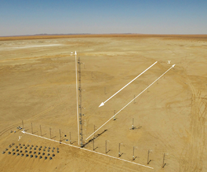
The high-Reynolds-number particle-laden two-phase flow data are obtained from long-term observations of aeolian sandstorms in ASLs performed at the QLOA site in western China. The QLOA shown in figure 1(a) was established on the flat dry lakebed of Qingtu Lake located between the Tenger Desert and the Badain Jaran Desert. The strong northwest monsoons and aeolian sandstorms moving southward pass by this area in the spring, which provides favourable conditions for observations. The QLOA consists of streamwise, spanwise and wall-normal arrays and thus can perform synchronous multi-point measurements of the three-dimensional turbulent flow field for both particle-laden and particle-free flows. More details regarding the experimental set-up at the QLOA site can be found in Wang & Zheng (Reference Wang and Zheng2016). The fluctuating velocity signals and sand concentration data employed in the present work were derived from the wall-normal array consisting of 11 pairs of velocity and sand concentration probes spaced logarithmically from  $z=0.9$ to 30 m (where $z$ denotes the wall-normal distance). Each pair of velocity and sand concentration probes was placed at the same height, as shown by the schematic in figure 1(b). The three components of the wind velocity and the temperature were measured by sonic anemometers (Campbell CSAT3B) with a sampling frequency of 50 Hz. Different from optical measurement methods such as particle image velocimetry, which is a huge challenge in multi-phase flow measurements that typically require optical method and particle size discrimination (Matinpour et al. Reference Matinpour, Bennett, Atkinson and Guala2019; Petersen, Baker & Coletti Reference Petersen, Baker and Coletti2019), the sonic anemometer estimates the velocity based on the time difference method (Horst & Oncley Reference Horst and Oncley2006), without effects from scattered signals by aerosols and, in this case, sand particles. Therefore, the sonic anemometer is widely used to measure the particle-laden flow in the ASL (Li Reference Li2013). The sand concentration was measured by an aerosol monitor (TSI, DUSTTRACK II-8530-EP) for particles with sizes less than 10 $\mathrm {\mu }$m (PM10) with a sampling frequency of 1 Hz. Meanwhile, to collect the horizontally transported sand particles during the sandstorm, the aeolian sand samplers (detailed in Dong et al. Reference Dong, Man, Luo, Qian, Wang, Zhao, Liu, Zhu and Zhu2010; Wang, Gu & Zheng Reference Wang, Gu and Zheng2020) were deployed independently at eight heights (0.9 m, 2.5 m, 5 m, 8.5 m, 10.24 m, 14.65 m, 20.96 m and 30 m) in the wall-normal array (as shown by the green up-pointing triangles in figure 1b). The sand particles collected by the sand sampler (instead of the DUSTTRACK) were analysed by a commercial standard sieve analyser (MicrotracS3500) to obtain the particle size distribution at different wall-normal locations.

Figure 1. (a) Photograph of the QLOA. (b) Schematic of the locations of the various probes in the wall-normal and spanwise arrays that are used in this study.
In addition, measurements below 0.9 m (0.03–0.5 m) were conducted in 2021 to acquire higher local mass loading than that further from the wall. The fluctuating streamwise velocity was measured by the outdoor hot-wire anemometer (ComfortSense-54T35 device from Dantec) which has a smaller probe volume (overall length of 0.3 m and shaft diameter of 0.01 m) compared with the sonic anemometer (0.6 m in length, 0.12 m in width and 0.43 m in height) and thus is more suitable for the near-wall measurement. The particle number information was acquired by the sand particle counter (SPC-91, Niigata Electric, previously used in Mikami Reference Mikami2005; Shao & Mikami Reference Shao and Mikami2005; Ishizuka et al. Reference Ishizuka, Mikami, Leys, Yamada, Heidenreich, Shao and McTainsh2008) which covers 64 particle size groups ranging from 30 to 480  $\mathrm {\mu }$m (a larger range of measurable particle sizes than that of DUSTTRACK) since the particles in the near-wall wind-blown sand two-phase flow are larger in diameter. The sampling frequency of both hot-wire and SPC are 1 Hz.
In the QLOA site, a soil crust is formed after rain due to the large salt content. Afterwards, the surface crust is gradually eroded, and eventually, a soft sandy surface is formed. This different degree of surface crust makes the sand concentration significantly different under the condition of a similar wind velocity. Even in the same sandstorm event, there may be significant differences in the sand concentration when a steady wind gradually develops. Taking a sandstorm with a duration of approximately 15 h from 12:00 on 16 April 2016 to 03:00 the next day as an example, figures 2(a) and 2(b) plot the corresponding streamwise velocity  $U$ and PM10 concentration $C_{{PM}10}$ measured at $z = 0.9$ m. Figure 2 shows that the wind velocity increases progressively towards a plateau with a mean velocity of approximately 10 m s $^{-1}$. However, the PM10 concentration decreases from approximately 1.3 mg m $^{-3}$ to near zero, while the wind velocity remains steady. This special experimental condition makes it possible to investigate the amplitude modulation under a large range of sand concentrations. It is noted that only approximately constant velocity and sand concentration data without drastic changes in mean value (as shown in the illustration in figure 2) are analysed in the present work. The observations were conducted at the QLOA site over a duration of more than 7000 h, and large amounts of particle-laden two-phase flow experimental data were obtained.

Figure 2. Streamwise velocity  $U$ (a), PM10 concentration $C_{{PM}10}$ (b) and the Monin–Obukhuv stability parameter $z/L$ (c) at $z=0.9$ m during the aeolian sandstorm process from 12:00 on 16 April 2016 to 03:00 the next day. Shaded areas with different colours are time series of 4 h data that are included in table 1, and these time series are magnified in the illustrations by lines with corresponding colour.
2.2. Data processing
Complex and uncontrollable field environmental conditions are inherent in these types of ASL measurements, thus specific selection and pre-processing are conducted on the raw data to obtain reliable datasets for the following analysis. According to the standard practice in the analysis of ASL data (Wyngaard Reference Wyngaard1992), the observational data were divided into multiple hourly time series to obtain converged statistics (Hutchins et al. Reference Hutchins, Chauhan, Marusic, Monty and Klewicki2012; Liu, Bo & Liang Reference Liu, Bo and Liang2017a). The data processing includes correction for the wind direction (Wilczak, Oncley & Stage Reference Wilczak, Oncley and Stage2001), steady wind selection (judged by the non-stationary index provided in Foken et al. Reference Foken, Gockede, Mauder, Mahrt, Amiro and Munger2004), thermal stability judgment (Monin & Obukhov Reference Monin and Obukhov1954) and de-trending (Hutchins et al. Reference Hutchins, Chauhan, Marusic, Monty and Klewicki2012), which is consistent with Hutchins et al. (Reference Hutchins, Chauhan, Marusic, Monty and Klewicki2012) and Wang & Zheng (Reference Wang and Zheng2016).
The  $x$-axis built into the sonic anemometer is not always along the incoming wind direction although it was installed to align with the prevailing wind direction. To acquire the actual three components of velocities, the wind direction correction is performed as
 $$\begin{gather} U=U_0 \cos (\alpha)+V_0 \sin (\alpha), \end{gather}$$
 $$\begin{gather}V=V_0 \cos (\alpha)-U_0 \sin (\alpha), \end{gather}$$
where  $U_0$ and $V_0$ are the raw streamwise and spanwise velocity components in the anemometer coordinate, $U$ and $V$ are the actual streamwise and spanwise velocities after correction and $\alpha = \arctan (\overline {v_0} /\overline {u_0})$ is the wind direction. The vertical velocity $W$ does not need to be corrected because the sonic anemometer was levelled during installation.
To acquire datasets with steady wind, the non-stationary index provided in Foken et al. (Reference Foken, Gockede, Mauder, Mahrt, Amiro and Munger2004) is employed, which is calculated as
 \begin{equation} IST=|(CV_m - CV_{1h})/CV_{1h}|\times 100\,\%,\end{equation}
where  $CV_m = \sum _{i = 1}^{12}CV_i /12, CV_i$ is the local streamwise velocity variance for every 5 min in 1 h and $CV_{1h}$ is the overall variance of the streamwise velocity for 1 h. Following Foken et al. (Reference Foken, Gockede, Mauder, Mahrt, Amiro and Munger2004), the high-quality data condition of $IST < 30\,\%$ is adopted to select the steady wind datasets. In addition, this criterion is also applied to the sand concentration data to ensure that the duration of each dataset is chosen for stationarity based on sand concentration as well.
The Monin–Obukhuv stability parameter  $z/L$ (Stull Reference Stull1988; Metzger, McKeon & Holmes Reference Metzger, McKeon and Holmes2007) is used to characterize the thermal stability, which is defined as
 \begin{equation} z/L={-}\frac{\kappa zg\overline{w\theta}}{\bar{\theta}U_\tau^3},\end{equation}
where  $L$ is Obukhov length, $\kappa = 0.41$ is the Kármán constant according to the ASL study of Marusic et al. (Reference Marusic, Monty, Hultmark and Smits2013), $g$ is the gravitational acceleration, $\bar {\theta }$ is the average temperature, $\overline {w\theta }$ is the wall-normal heat flux obtained from the covariance between the temperature fluctuations $\theta$ and the vertical velocity fluctuations $w$ and $U_\tau$ is the friction velocity which is estimated as $U_\tau =\sqrt {-\overline {uw}}$ at $z = 2.5$ m following Hutchins et al. (Reference Hutchins, Chauhan, Marusic, Monty and Klewicki2012) and Li & Neuman (Reference Li and Neuman2012). The resulting $z/L$ in a whole sandstorm process is shown in figure 2(c).
It is seen that, at the beginning of the sandstorm,  $z/L$ exhibits small negative values, indicating that the ASL is unstably stratified and buoyancy would enhance the turbulence production. As the wind speed develops to become steady, $z/L$ reduces to values that are close to zero, indicating that the ASL is nearly neutrally stratified and thus analogous to a canonical TBL. At the decay stage of the sandstorm, $z/L$ increases to large positive values, which suggests that the ASL is stably stratified and the turbulence is weakened. To investigate the particle effects on amplitude modulation in particle-laden flows where thermal stability effects can be considered negligible, datasets in the neutral regime should be selected. A criterion of $|z/L| \leqslant 0.04$ for a neutral stratification condition is confirmed to be applied to the particle-laden case by analysing the variations of the basic statistics and amplitude modulation coefficient vs $|z/L|$ using datasets with similar particle concentrations and different thermal stabilities (details of which are presented in the Appendix). This criterion is stricter than that of $|z/L|<0.1$ in the existing studies (Högström Reference Högström1988; Högström, Hunt & Smedman Reference Högström, Hunt and Smedman2002; Metzger et al. Reference Metzger, McKeon and Holmes2007).
In addition, the de-trending manipulation proposed in Hutchins et al. (Reference Hutchins, Chauhan, Marusic, Monty and Klewicki2012) is employed to remove the effects of the background turbulent characteristics that are directly regulated by the weather conditions and/or atmospheric motions. Due to the global nature of the weather conditions, any events registered across the entire measurement domain can be regarded as weather related. Therefore, the streamwise velocity fluctuations synchronously measured by all of the sonic anemometers over the whole array were averaged together to extract the long-term trends which are weather related (Hutchins et al. Reference Hutchins, Chauhan, Marusic, Monty and Klewicki2012). A low-pass filter with a cutoff wavelength of  $20\delta$ is used to obtain the broad trend. Then, the synoptic waves were subtracted from the raw data to leave just the turbulent fluctuations for further analysis.
After applying the data processing procedure, 24 h of data with similar Reynolds numbers ( $(3.85\pm 1.35)\times 10^{6}$) and different sand concentrations spanning almost three orders of magnitude in $\varPhi _{m}$ are subsequently analysed in this study, as listed in table 1. According to Mathis et al. (Reference Mathis, Hutchins and Marusic2009a) and Liu et al. (Reference Liu, Wang and Zheng2019), the amplitude modulation exhibits an approximate Reynolds-number independence over three orders of magnitude in $Re_{\tau }$ when outer scaled with $z/\delta$. Therefore, the outer-scaled $z/\delta$ unit was employed in the subsequent analysis to minimize the Reynolds-number effects. The ASL thickness $\delta$ at the QLOA site estimated by Wang & Zheng (Reference Wang and Zheng2016), Liu et al. (Reference Liu, Bo and Liang2017a) and Liu et al. (Reference Liu, Wang and Zheng2019) based on the streamwise turbulent intensity formula provided in Marusic et al. (Reference Marusic, Monty, Hultmark and Smits2013) was 106 $-$191 m with an average of approximately 150 m. Moreover, the value of $\delta$ determined by the horizontal wind speed data ( $>30$ m) collected by Doppler lidar in 2021 suggests that the $\delta$ under different $\varPhi _{m}$ conditions is kept within the range of $142 \pm 23$ m. Thus, the ASL thickness $\delta$ is adopted as 150 m (considering that the exact choice of $\delta$ does not affect the maximum amplitude modulation coefficient between multi-scale turbulent motions and the following analysis does not involve the Reynolds-number effects). The kinematic viscosity $\nu$ was calculated by the barometric pressure and the temperature at the QLOA site (Tracy, Welch & Porter Reference Tracy, Welch and Porter1980).
Table 1. Key information relating to the datasets in the particle-laden ASL. The last column is  $\varPhi _{m}$ at the wall-normal distance $z = 0.9$ m (datasets 1–14) and $z = 0.03$ m (datasets 15–24).

2.3. Two-phase flow parameters
The last column in table 1 provides the average particle mass loading  $\varPhi _{m}$ at a wall-normal location. Here, $\varPhi _{m}$ is estimated from the measured data of DUSTTRACK or SPC. For DUSTTRACK, the concentration of particles with sizes less than 10 $\mathrm {\mu }$m (denoted by $C_{{PM10}}$) is measured. Therefore, to obtain the total mass loading of particles of all sizes, it is necessary to acquire the percentage of PM10 in all particles with different sizes. The particle size distribution can be obtained by analysing the collected sand particles with a commercial standard sieve analyser (MicrotracS3500), where the sand particles were collected by the aeolian sand samplers placed at different wall-normal locations. Figure 3(a) shows the resulting particle size distribution. It is seen in figure 3(a) that the diameters of sand particles present a distribution deviating slightly from a Gaussian distribution. The sand grain diameter varies from 4 to 400 $\mathrm {\mu }$m, with the average diameters decreasing from 105 to 70 $\mathrm {\mu }$m vs the wall-normal distance. The particle size distribution during the different events is basically the same due to the local sand source. The percentage of PM10 (denoted by $P_{{PM10}}$) at different heights is shown in the illustration in figure 3(a). As expected, $P_{{PM10}}$ increases with $z/\delta$. Based on $P_{{PM10}}, \varPhi _{m}$ can be estimated as
 \begin{equation} \varPhi _{m}=\frac{\varPhi_{m}^{{PM10}}}{P_{{PM10}}} =\frac{\overline{C_{{PM10}}}}{\rho_{f}P_{{PM10}}},\end{equation}
where  $\varPhi _{m}^{{PM10}}$ is the average mass loading of particles with sizes less than 10 $\mathrm {\mu }$m (i.e. PM10 mass loading), $\rho _{f} \approx$ 1.26 kg m $^{-3}$ is the air density and the over bar denotes the time average.

Figure 3. (a) Particle diameter distribution of the sand grains at different wall-normal locations, where the illustration shows the percentage of particles with diameters smaller than 10  $\mathrm {\mu }$m. (b) Variation in $\varPhi _{m}$ with the outer-scaled wall-normal distance. It is noted that ‘No.’ refers to the sample sets in table 1.
For SPC, the large range of measurable particle sizes makes it possible to capture almost all of the near-wall sand grains. Following Shao & Mikami (Reference Shao and Mikami2005), the particle mass flux measured by SPC is calculated as
 \begin{equation} q(t)=\sum_{i=1}^{64}q_{i}(t)=\sum_{i=1}^{64}\frac{{\rm \pi} \rho_{p}d_{i}^{3}N_{i}(t)}{6S{\rm \Delta} T}, \end{equation}
where  $\rho _{p}$ = 2650 kg m $^{-3}$ is the particle density, $N_{i}$ is the number of particles of size $d_i$ during ${\rm \Delta} T, {\rm \Delta} T$ is time interval and $S = 5 \times 10^{-5}$ m $^{2}$ is the measurement area of the SPC. Then, based on $q(t), \varPhi _{m}$ can be estimated as
 \begin{equation} \varPhi_{m}=\frac{\overline{q(t)}}{\bar{u}\rho_{f}},\end{equation}
where  $\bar {u}$ is the local mean velocity at the corresponding wall-normal distance.
The resulting  $\varPhi _{m}$ at different measurement heights are plotted in figure 3(b). It is seen that, for all of the data with different sand concentrations, $\varPhi _{m}$ decreases progressively with the outer-scaled wall-normal distance. The variation of $\varPhi _{m}$ with $z/\delta$ is systematic and follows an approximately linear decrease in the double logarithmic coordinates. This trend is consistent with the previously documented results of PM10 concentration vertical profile in McGowan & Clark (Reference McGowan and Clark2008) and Panebianco, Mendez & Buschiazzo (Reference Panebianco, Mendez and Buschiazzo2016) and mass flux profile in Panebianco, Buschiazzo & Zobeck (Reference Panebianco, Buschiazzo and Zobeck2010).
Following Li et al. (Reference Li, Lim, Berk, Abraham, Heisel, Guala, Coletti and Hong2021), the turbulence dissipation rate can be estimated as
 \begin{equation} \varepsilon=\sigma ^3/l,\end{equation}
where  $\sigma$ is the root mean square of the streamwise velocity fluctuation and $l \propto z = \kappa z$ is based on a local scale (Tardu Reference Tardu2011). The characteristic length and time scale of the fluid is usually taken as the Kolmogorov scale ( $\eta, \tau _\eta$) or the integral scale ( $L, \tau _ L$). The Kolmogorov length and time scale is estimated as
 $$\begin{gather} \eta=(\nu ^3/\varepsilon)^{1/4}, \end{gather}$$
 $$\begin{gather}\tau _\eta = (\nu/\varepsilon)^{1/2}. \end{gather}$$
The integral time scale  $\tau _L$ and the length scale $L$ are calculated from the temporal auto-correlation function $R_{uu}$ of the streamwise velocity fluctuations (Emes et al. Reference Emes, Arjomandi, Kelso and Ghanadi2019; Li et al. Reference Li, Lim, Berk, Abraham, Heisel, Guala, Coletti and Hong2021), i.e.
 \begin{equation} R_{uu} (\tau) = \frac{\overline{u(t)u(t+\tau)}}{\sigma _{t}\sigma_{t+\tau}}, \end{equation}
where  $t$ is the measure time, and $\tau$ is the temporal lag. The corresponding integral time and length scale are given as
 $$\begin{gather} \tau _L = \int_{0}^{T_{0}}R_{uu}(\tau) \, {\rm d} \tau, \end{gather}$$
 $$\begin{gather}L = \bar{u} \tau _L, \end{gather}$$
where  $T_0$ is the first zero-crossing point of the auto-correlation function.
The particle response time  $\tau _p$ can be given as (Wang & Stock Reference Wang and Stock1993)
 \begin{equation} \tau_p=\rho_p d_p ^2 /18\rho_{f} \nu,\end{equation}
where  $d_p$ denotes the average particle diameter at each wall-normal location. Thus, the Stokes numbers $St$ based on the Kolmogorov time scale, integral time scale and viscous inner time scale are estimated as
 $$\begin{gather} St_\eta=\tau_p/\tau_{\eta}, \end{gather}$$
 $$\begin{gather}St_L=\tau_p/\tau_{L}, \end{gather}$$
 $$\begin{gather}St^{+}=\tau_p u_{\tau}^{2}/\nu, \end{gather}$$
respectively. Moreover, the Froude number is defined as (Bernardini Reference Bernardini2014)
 \begin{equation} Fr=u_{\tau}/\tau_{p}g.\end{equation}
The resulting key fluid and particle parameters related to the particle-laden flow are listed in table 2, which suggests that all cases in table 1 fall into these ranges.
Table 2. Key information of fluid and particles in particle-laden flow.

2.4. Basic statistics
Hutchins et al. (Reference Hutchins, Chauhan, Marusic, Monty and Klewicki2012) and Wang & Zheng (Reference Wang and Zheng2016) confirmed that near-neutral particle-free ASL flows exhibit scaling laws that are generally representative of the canonical zero-pressure-gradient TBL, and thus can be used in studies of high-Reynolds-number wall-bounded turbulent flows, based on observational data in the Surface Layer Turbulence and Environmental Science Test (SLTEST) site and QLOA site. It is prudent to analyse particle effects on the basic statistics in particle-laden ASL flows. Figures 4(a)–4(c) show respectively the mean velocity profile, the streamwise turbulent intensity and the Reynolds shear stress for the neutral particle-laden ASL datasets used in the present work. It is seen in figure 4(a) that the mean velocity profiles for all of the datasets with different  $\varPhi _{m}$ follow the predicted log–linear behaviours, but there is an increasing downward shift with the $\varPhi _{m}$ in the present ASL data compared with that for a hydraulically smooth wall ( $k_s^+ < 2.25$). The downward shift trend by particles is consistent with the results in Li et al. (Reference Li, Wang, Liu, Chen and Zheng2012) and Lee & Lee (Reference Lee and Lee2019). Nevertheless, the equivalent sand grain roughness heights $k_s^+$ are approximately less than 80, which could still be in the transitionally rough regime ( $2.25 \leq k_x^+ \leq 90$) (Ligrani & Moffat Reference Ligrani and Moffat1986) and consistent with the results for the desert surface (Metzger et al. Reference Metzger, McKeon and Holmes2007; Guala, Metzger & McKeon Reference Guala, Metzger and McKeon2010; Hutchins et al. Reference Hutchins, Chauhan, Marusic, Monty and Klewicki2012). Figure 4(b) indicates that the streamwise turbulent intensity at low $\varPhi _{m}$ is in good agreement with the existing similarity formation proposed by Marusic et al. (Reference Marusic, Monty, Hultmark and Smits2013). As $\varPhi _{m}$ increases, the turbulent intensity increases, which is consistent with the findings in Li & Neuman (Reference Li and Neuman2012), Li et al. (Reference Li, Wang, Liu, Chen and Zheng2012) and Wang et al. (Reference Wang, Gu and Zheng2020). In addition, the Reynolds shear stresses in laden cases attain an approximate plateau like the unladen case in figure 4(c). This indicates that the ‘constant stress’ layer recorded in Townsend (Reference Townsend1976) still exists in the present sand-laden flow, where the relation $-\overline {uw}=U_\tau ^2$ is still satisfied. Therefore, it is suitable to estimate the friction velocity by the plateau value in the Reynolds shear stress, as is done in this study. It is for this reason that the Reynolds shear stress normalized by $U_\tau$ exhibits a plateau value of 1, which is consistent with the similarity formulation in Chauhan (Reference Chauhan2007) and Nagib & Chauhan (Reference Nagib and Chauhan2008).

Figure 4. Variations of mean streamwise velocity profile (a), streamwise turbulent kinetic intensity (b) and Reynolds shear stress (c) with the inner-scaled wall-normal distance  $z^+$. Hollow circles and yellow filled circles are the present results (nos. 1, 5, 9), hollow triangles are the result in Hutchins et al. (Reference Hutchins, Chauhan, Marusic, Monty and Klewicki2012) at $Re_\tau = 7.7 \times 10^{5}$. Grey dashed lines in (a), $\overline {u}^+ = 1/0.41ln(z^+) + 5.0-{\rm \Delta} \overline {u}^+$; $k_s^+$ is the equivalent sand grain roughness heights. Black dashed lines in (b) and dotted-dashed lines in (c) are the similarity formulations provided in Marusic et al. (Reference Marusic, Monty, Hultmark and Smits2013) and Chauhan (Reference Chauhan2007) at the Reynolds number corresponding to the experimental data.
3. Particle effects on turbulent kinetic intensity distribution
There is a series of coherent structures with different length scales that inhabit the high-Reynolds-number wall-bounded turbulence, where the LSMs and VLSMs are dominant in the outer region. Given that the particles enhance the turbulent intensity in two-phase flow, this section aims to explore whether the influence of particles is uniform at different scale structures; that is, whether the particles change the distribution of energy of different scale motions.
To gain insight into the influence of particles on the energy distribution in different scale turbulent motions, figures 5(a) and 5(b) show the pre-multiplied energy spectra of the streamwise velocity fluctuations  $k_{x}\varPhi _{uu}/U_{\tau }^{2}$ (where $k_{x}=2{\rm \pi} /\lambda _{x}$ is the streamwise wavenumber and $\varPhi _{uu}$ is the power spectral density) vs the streamwise wavenumber $k_{x}\delta$ at $z \approx 0.01\delta$ and $z \approx 0.02\delta$, respectively. The analysis of the pre-multiplied spectra follows the methods of Kim & Adrian (Reference Kim and Adrian1999), Vallikivi, Ganapathisubramani & Smits (Reference Vallikivi, Ganapathisubramani and Smits2015) and Wang & Zheng (Reference Wang and Zheng2016). The results from datasets with different $\varPhi _{m}$ are shown in figure 5 by different coloured lines for comparison, where black lines are the results for low $\varPhi _{m}$, blue lines are those for high $\varPhi _{m}$ and grey lines are the particle-free flow results in Wang & Zheng (Reference Wang and Zheng2016).

Figure 5. Pre-multiplied energy spectra of the streamwise velocity fluctuations  $k_{x}\varPhi _{uu}/U_{\tau }^{2}$ vs the streamwise wavenumber $k_{x}\delta$ at (a) $z \approx 0.01\delta$ and (b) $z \approx 0.02\delta$ from datasets with different particle mass loading: black lines, low $\varPhi _{m}$ (no. 1 and no. 2); blue lines, high $\varPhi _{m}$ (no. 11 and no. 13). The grey lines are the particle-free results in Wang & Zheng (Reference Wang and Zheng2016).
It is seen from the low  $\varPhi _{m}$ results in figure 5 that the spectral peak in the lower wavenumber region associated with the VLSMs is more distinct than the higher wavenumber peak associated with the LSMs, which suggests more dominant VLSMs in high-Reynolds-number flows than that in lower-Reynolds-number cases. This is as observed by the single-phase flow experimental results in Vallikivi et al. (Reference Vallikivi, Ganapathisubramani and Smits2015), and the profiles for low $\varPhi _{m}$ agree well with the particle-free ASL result provided in Wang & Zheng (Reference Wang and Zheng2016). The consistency indicates that the low $\varPhi _{m}$ data exhibit almost the same properties as are typical in the particle-free flow. In addition to a distinct peak associated with the VLSMs, the pre-multiplied energy spectra with high $\varPhi _{m}$ in figure 5 show a significant difference from the low $\varPhi _{m}$ results. The magnitude of the energy spectra in flows with large $\varPhi _{m}$ is much larger than that with very small values of $\varPhi _{m}$, while the positions of the distinct peak remain almost unchanged. The unchanged peak position suggests that the scale of the most energetic structure does not change with the presence of particles. However, the increase of the magnitude of the energy spectra seems to be the overall uplift of the profile, with signs that the uplift is more pronounced in the higher wavenumber region than in the lower wavenumber region. This implies that the energetic signature of different scale structures is enhanced by particles in the two-phase flow, but the degree of enhancement for large-scale and small-scale components may be different.
Therefore, to further investigate the influence of particles on the kinetic energy of different scale motions, especially the VLSMs, figure 6 plots the streamwise turbulent kinetic energy of the VLSMs with length scales larger than 3 $\delta$ (Guala et al. Reference Guala, Hommema and Adrian2006; Balakumar & Adrian Reference Balakumar and Adrian2007) and the total streamwise turbulent kinetic energy in flows with different $\varPhi _{m}$. The particle-free flow results that available in Wang & Zheng (Reference Wang and Zheng2016) are also plotted in figure 6 for comparison. It is seen in figure 6 that the streamwise turbulent kinetic energy remains almost invariant when $\varPhi _{m}$ is small, and the previously reported values in the particle-free flow (Wang & Zheng Reference Wang and Zheng2016) are basically consistent with the trend. With increasing $\varPhi _{m}$, the turbulent kinetic energy of both the total and the VLSMs increases systematically with $\varPhi _{m}$, when $\varPhi _{m}$ is larger than approximately $O(10^{-5})$. To quantify the rate of the increase with $\varPhi _{m}$, a log–linear equation is fitted to the experimental data (shown by dashed lines), and the slope can subsequently be obtained. The simple log–linear fit is just to quantify the growth rate, regardless of the specific functional form. It is interesting to find that the slope of the total turbulent kinetic energy increasing with $\varPhi _{m}$ is approximately 19.5, which is much larger than the slope for the kinetic energy of VLSMs (approximately 6.9). The difference in the rate of increase indicates that, although the addition of particles in the two-phase flow enhances the turbulent kinetic energy of the VLSMs, the total turbulent kinetic energy has a more significant increase. This provides further evidence supporting that there are some differences in the influence of particles on the kinetic energy of turbulent motion at different scales. Compared with the total kinetic energy, the kinetic energy of VLSMs is less enhanced by particles, suggesting a weakened dominance of VLSMs in the two-phase flow. In addition, the variation of turbulent kinetic energy in particle-laden flow is different from that in Rogers & Eaton (Reference Rogers and Eaton1991), but consistent with the results in Wang et al. (Reference Wang, Gu and Zheng2020), which may be related to the multiple particle sizes.

Figure 6. Changes in the turbulent kinetic energy (TKE) of the total and VLSMs with scales larger than  $3\delta$ vs $\varPhi _{m}$ (nos. 1–14) at $z\approx 0.01\delta$. The lines are the fitting curves. The open circle and square symbols denote the particle-free ASL results in Wang & Zheng (Reference Wang and Zheng2016).
More generally, figure 7 presents the cumulative energy fraction of the streamwise velocity fluctuations as a function of wavelength ( $\lambda _{c}/\delta$). Here, $E_{\lambda _{x}<\lambda _{c}}$ is the cumulative contribution of the small-scale turbulent motion components with wavelengths from $\lambda _{c}$ to 0 (shown in figure 7 by blue), and $E_{\lambda _{x}>\lambda _{c}}$ is the contribution from the large-scale components with wavelengths greater than $\lambda _{c}$ (shown in figure 7 by black). The comparison of the results in particle-laden flows with large $\varPhi _{m}$ (shown by the dashed line) and those with low $\varPhi _{m}$ (shown by the solid line) shows that the energy fraction of the large-scale component is reduced by the addition of sand particles, while the energy fraction of the small-scale component is increased (which is more significant as compared with the particle-free TBL results in Guala et al. Reference Guala, Hommema and Adrian2006; Balakumar & Adrian Reference Balakumar and Adrian2007). This phenomenon indicates that the addition of particles not only increases the energy of the VLSMs but also more significantly increases the energy of small-scale motions. That is, the particles change the distribution of energy between multi-scale turbulent motions: the energy fraction of the large-scale component is reduced, while the small-scale component is enhanced. The reduction of the energy fraction of the VLSMs in the particle-laden flow may weaken the influence on the small-scale motions, thereby reducing the amplitude modulation effect.

Figure 7. Cumulative streamwise kinetic energy fraction associated with structures with wavelengths greater than  $\lambda _{c}$ (left vertical axis and bottom abscissa, shown by black) and less than $\lambda _{c}$ (right vertical axis and top abscissa, shown by blue) at $z\approx 0.01\delta$. The solid lines are the average results for datasets with low $\varPhi _{m}$ ( $<1.33\times 10^{-5}$, nos. 1–2), and the dashed lines are those with high $\varPhi _{m}$ ( $> 1.5\times 10^{-4}$, nos. 7–14). The red, green and yellow lines are the particle-free results in Balakumar & Adrian (Reference Balakumar and Adrian2007) and Guala et al. (Reference Guala, Hommema and Adrian2006), respectively.
It is well known that the coherent structure essentially represents a three-dimensional region of a flow over which at least one fundamental flow variable (such as velocity, temperature or pressure) exhibits an obvious correlation with itself or with another variable over a large range of space and time (Robinson Reference Robinson1991). Moreover, the hairpin vortex packet model proposed by Kim & Adrian (Reference Kim and Adrian1999) and Adrian et al. (Reference Adrian, Meinhart and Tomkins2000) suggests that LSMs/VLSMs are created by the coherence of alignment between multiple hairpin vortices. It can be seen that the maintenance of large-scale coherent structures is closely related to the coherence between fluids. On the one hand, the disturbance of the sand particles (with gravity and large density) enhances the streamwise TKE in the particle-laden flow. On the other hand, the particle disturbance may also break the coherence of the fluctuating signals at different positions in the flow field.
This result can be confirmed by the time-lag auto-correlation of the streamwise velocity fluctuations shown in figure 8 for both the large  $\varPhi _{m}$ case and the particle-free case. The relatively reliable average results of $R_{uu}$ for particle-free datasets available in Liu et al. (Reference Liu, Wang and Zheng2019) and particle-laden datasets with $\varPhi _{m} > 1.5\times 10^{-4}$ are presented in figure 8 to reduce the ASL experimental scatter. The corresponding standard deviation is approximately $\pm (0-0.058)$, which is shown in figure 8 by the shaded area. The abscissa in figure 8 is shown in length units by converting the temporal lead/lag ( ${\rm \Delta} t$) using Taylor's hypothesis of frozen turbulence ( ${\rm \Delta} x = \bar {u}{\rm \Delta} t$, where $\bar {u}$ is the convection velocity taken as the local mean). Figure 8 shows that, at the same streamwise separation, the absolute value of the correlation coefficient $R_{uu}$ is generally reduced in two-phase flows with large $\varPhi _{m}$ (shown by the blue solid line) although with experimental scatter. A characteristic length scale from the time-lag auto-correlation can be extracted by a nominal threshold of $R_{uu}$. A small positive value is usually chosen as the threshold, such as $R_{uu}=0.05$ (Hutchins, Hambleton & Marusic Reference Hutchins, Hambleton and Marusic2005), 0.1 (Dennis & Nickels Reference Dennis and Nickels2011) and 0.4 (Tomkins & Adrian Reference Tomkins and Adrian2003). In any case, the smaller $R_{uu}$ suggests a reduced correlation length scale. This finding indicates that sand particles weaken the coherence between fluids, and thus reduce the average scale of the coherent structures in the two-phase flow. Therefore, when the velocity fluctuations is cutoff at the same wavelength, more motions are divided into small-scale component, while fewer are divided into large-scale component. This makes the energy contained in the large-scale component decrease, while the energy contained in the small-scale component increases, as suggested in figure 7.

Figure 8. Time-lag streamwise velocity correlations ( $R_{uu}$) along the streamwise direction at $z \approx 0.01\delta$. The black solid line denotes the average results for particle-free datasets available in Liu et al. (Reference Liu, Wang and Zheng2019) and the blue solid line represents the average $R_{uu}$ for datasets with $\varPhi _{m}>1.5\times 10^{-4}$ (nos. 7–14). The grey and blue shaded areas are the standard deviation.
In summary, the analysis in this section indicates that sand particles enhance turbulence, but the degree of enhancement is different, the kinetic energy of VLSMs is less enhanced than the total kinetic energy. This changes the distribution of energy between multi-scale turbulent motions in the two-phase flow, the energy proportion of the large-scale component decreases while that of the small-scale component increases. Moreover, the addition of sand particles in the two-phase flow reduces the average scale of the coherent structures due to the weakened coherence between fluids, but hardly changes the scales of the most energetic structures.
4. Particle effects on amplitude modulation covariance
Given the change in the distribution of TKE in the particle-laden flow, especially the reduced large-scale energy proportion, it is logical then to consider their effect on the amplitude modulation of LSMs onto small scales, because the degree of amplitude modulation is closely related to the energy signature of the large-scale structures in the outer region (Mathis et al. Reference Mathis, Hutchins and Marusic2009a). The amplitude modulation covariance proposed by Bernardini & Pirozzoli (Reference Bernardini and Pirozzoli2011) is an unnormalized form of the amplitude modulation, which provides a better perception of the absolute importance of the modulation effect between large- and small-scale motions. Therefore, this section explores the particle effects on the amplitude modulation covariance.
The amplitude modulation covariance is defined as the covariance between the large-scale component of the fluctuating streamwise velocity signal  $u_{L}^{+}$ and the filtered envelope of the small-scale fluctuations $E_{L}(u_{S}^{+})$. When $u_L$ and $u_S$ are taken from two different wall-normal locations $z_1$ and $z_2$, it presents the inter-layer (or two-point) amplitude modulation covariance, which is calculated following the method provided in Bernardini & Pirozzoli (Reference Bernardini and Pirozzoli2011) and Tong, Duan & Li (Reference Tong, Duan and Li2022)
 \begin{equation} C_{AM}(z_1,z_2)= \overline{u_L^+(z_1)E_L(u_S^+(z_2))},\end{equation}
where the superscript  $+$ represents the inner-flow scaling normalized with the friction velocity $U_{\tau }$ and the kinematic viscosity $\nu$, for example, $u^{+}=u/U_{\tau }$, and $z^{+}=zU_{\tau }/\nu$. The large-scale $u_{L}^{+}$ and the small-scale components $u_{S}^{+}$ of the signals are obtained by applying Fourier filters to the raw fluctuating streamwise velocity $u^{+}$ signal with a nominal cutoff wavelength. The envelope of the small-scale components $E(u_{S}^{+})$ is extracted via the Hilbert transformation (Spark & Dutton Reference Spark and Dutton1972; Sreenivasan Reference Sreenivasan1985) to track the changes in the amplitude of these scales. However, $E(u_{S}^{+})$ tracks not only the large-scale modulation events due to the LSMs/VLSMs but also the small-scale variations in the carrier signal. Thus, the filtered envelope $E_{L}(u_{S}^{+})$ is employed by low-pass filtering the envelope at the same cutoff as the large-scale component to describe the modulation of small-scale motions. The inter-layer amplitude modulation covariance gives a perception of the absolute importance of the modulation effect at two different wall-normal locations ( $z_1, z_2$) (Bernardini & Pirozzoli Reference Bernardini and Pirozzoli2011), which reflects the occurrence of a top–down interaction between LSMs in the outer region and the small-scale motions in the inner region.
The inter-layer amplitude modulation covariance extracted from low  $\varPhi _{m}$ and high $\varPhi _{m}$ flows are plotted in figures 9(a) and 9(b), respectively. The nominal cutoff wavelength is adopted as the ASL thickness $\delta$ following Mathis et al. (Reference Mathis, Hutchins and Marusic2009a). It is seen from the main trend in figure 9(a) that the colour contour is asymmetric with respect to the diagonal line, being consistent with the high-Reynolds-number results in Bernardini & Pirozzoli (Reference Bernardini and Pirozzoli2011). The inter-layer amplitude modulation represents the effect of the outer region on the inner region, thus the region below the diagonal ( $z_1 > z_2$) is usually of most concern, and we do not discuss the results above the diagonal ( $z_1 < z_2$). Specifically, figure 9(a) shows an overall positive values of $C_{AM}(z_1,z_2)$ below the diagonal, and a distinct peak emerges on the bottom-right side of the map (located at approximately $z_1 \approx 0.1\delta$ and $z_2 \approx 0.02\delta$), that is, there is an off-diagonal peak as observed in Bernardini & Pirozzoli (Reference Bernardini and Pirozzoli2011). This indicates that at all of the measurement heights in the logarithmic region, the modulation is always positive when the large-scale modulating signal is located higher than the small-scale carrier signal (i.e. the top–down influence), where the LSMs near the top of the logarithmic region most significantly modulate the small scales near the mid-point of the logarithmic region. In the high $\varPhi _{m}$ case shown in figure 9(b), compared with the low $\varPhi _{m}$ case, the difference is mainly reflected in two aspects: one is that the position of the off-diagonal peak slightly shifts to the lower left; the other is that the magnitude of $C_{AM}(z_1,z_2)$ decreases. The shift of the peak position indicates that the positions of the modulating signals and the carrier signals with the most significant modulation move downwards in the particle-laden flow. For the decreased $C_{AM}(z_1,z_2)$, this may be caused by the decrease in the degree of correlation, or by the decrease in the fluctuation intensities of $u_{L}^{+}$ and $E_{L}(u_{S}^{+})$.

Figure 9. Inter-layer amplitude modulation covariance from the large-scale turbulent motions ( $\lambda _{x}>\delta$) at the wall-normal location $z_1$ onto the small-scale motions ( $\lambda _{x}<\delta$) at $z_2$. (a) Average results for data with low $\varPhi _{m}$ ( $< 1.33 \times 10^{-5}$, nos. 1–2); (b) those with high $\varPhi _{m}$ ( $> 1.5 \times 10^{-4}$, nos. 7–14).
To analyse the amplitude modulation between multi-scale turbulent motions, two variables  $\lambda _{cL}$ and $\lambda _{cS}$ are introduced in the decoupling procedure by Liu et al. (Reference Liu, Wang and Zheng2019). Here, $\lambda _{cL}$ is employed as the low-pass filter cutoff wavelength to obtain the large-scale component (wavelength $\lambda _{x}>\lambda _{cL}$), and $\lambda _{cS}$ is adopted as the high-pass filter cutoff wavelength to obtain the small-scale component ( $\lambda _{x}<\lambda _{cS}$). This can be given as
 $$\begin{gather} u_{L}^{+}=u^{+}|(\lambda_{x}>\lambda_{cL}), \end{gather}$$
 $$\begin{gather}u_{S}^{+}=u^{+}|(\lambda_{x}<\lambda_{cS}). \end{gather}$$
Correspondingly, the Hilbert transformation is applied on the small-scale component to extract the envelope, and the filtered envelope is obtained as
 \begin{equation} E_{L}(u_{S}^{+})=E(u_{S}^{+})|(\lambda_{x}>\lambda_{cL}),\end{equation}
to describe the varying amplitude of the small-scale component caused by large-scale fluctuations. Then, the amplitude modulation covariance between multi-scale turbulent motions is calculated as
 \begin{equation} C_{AM}(\lambda_{cL},\lambda_{cS})= \overline{u_L^{+}(\lambda_{x}>\lambda_{cL}) E_L(u_{S}^{+}(\lambda_{x}<\lambda_{cS}))}, \end{equation}
where  $u_L$ and $u_S$ are taken from the same wall-normal location.
The contours of the multi-scale amplitude modulation covariance  $C_{AM}(\lambda _{cL},\lambda _{cS})$ vs the length scales of the large-scale components ( $\lambda _{x}> \lambda _{cL}$) and small-scale components ( $\lambda _{x}< \lambda _{cS}$) in low and high $\varPhi _{m}$ cases are shown in figures 10(a) and 10(b), respectively, to provide an absolute rather than a normalized value of the amplitude modulation between multi-scale turbulent motions. It can be seen in figure 10(a) that the peak of $C_{AM}(\lambda _{cL},\lambda _{cS})$ can still be found at different scale turbulent motions, although the single-point modulation covariance estimated by establishing a nominal cutoff wavelength to divide the large-scale and small-scale components is relatively small (as shown by the diagonal line in figure 9). The peak in the low $\varPhi _{m}$ case is concentrated around $\lambda _{cL}\approx \lambda _{cS}\approx 2\delta$. This indicates that there is a significant modulation effect between different scales of turbulent motions at the same wall-normal location, but it only exists in some specific motions. However, the overall trend of the contour in figure 10(a) is quite different from the contour of multi-scale amplitude modulation coefficient provided in Liu et al. (Reference Liu, Wang and Zheng2019). This may be caused by the different distributions of the fluctuation intensities of $u_{L}^{+}$ and $E_{L}(u_{S}^{+})$ at different scales.

Figure 10. Colour contour maps showing the variations in the amplitude modulation covariance  $C_{AM}$ ( $\lambda _{cL}, \lambda _{cS}$) with the length scales of the large-scale ( $\lambda _{x} > \lambda _{cL}$) and small-scale ( $\lambda _{x} < \lambda _{cS}$) components at $z\approx 0.01\delta$. (a) Average results for data with low $\varPhi _{m}$ ( $< 1.33 \times 10^{-5}$, nos. 1 $-$2); (b) those with high $\varPhi _{m}$ ( $> 1.5 \times 10^{-4}$, nos. 7 $-$14).
In addition, the comparison of high  $\varPhi _{m}$ results in figure 10(b) and low $\varPhi _{m}$ results shows that the most significant difference is the attenuated magnitude of $C_{AM}(\lambda _{cL},\lambda _{cS})$ in the high $\varPhi _{m}$ case, making the peak value less obvious. This suggests a suppressed amplitude modulation covariance between multi-scale turbulent motions, agreeing with the damping tendency of inter-layer amplitude modulation covariance shown in figure 9.
It is noted that the amplitude modulation covariance is a dimensional quantity, which is affected by the fluctuation intensities of  $u_{L}^{+}$ and $E_{L}(u_{S}^{+})$. Therefore, to examine the distribution of their coupled fluctuation intensity for multi-scale turbulent motions and different wall-normal positions, figures 11(a)–11(d) show the contours of the root-mean-square product of $u_{L}^{+}$ and $E_{L}(u_{S}^{+})$ in both low $\varPhi _{m}$ and high $\varPhi _{m}$ flows. This root-mean-square product actually represents the energetic signature of the large-scale components since $E_{L}(u_{S}^{+})$ tracks the large-scale modulation events caused by $u_{L}^{+}$. The contours for $u_{L}^{+}$ and $E_{L}(u_{S}^{+})$ residing at different flow layers $z_{1}$ and $z_{2}$ are shown in figures 11(a) and 11(b). Figure 11(a) indicates that the distribution of the root-mean-square product is quite uniform, suggesting a negligible variation of the large-scale kinetic energy with the wall-normal distance. This is consistent with the particle-free results in TBL (Balakumar & Adrian Reference Balakumar and Adrian2007), pipe (Guala et al. Reference Guala, Hommema and Adrian2006) and channel (Duan et al. Reference Duan, Chen, Li and Zhong2020) flows. The distribution of the root-mean-square product in the high $\varPhi _{m}$ flow shown in figure 11(b) is similar to that in the low $\varPhi _{m}$ case except for the increased magnitude. Therefore, the contour map of the inter-layer modulation covariance can reflect the distribution of the amplitude modulation degree in both particle-laden and unladen flows. However, the augmented energetic signature in the high $\varPhi _{m}$ case seems to imply a reduced correlation of $u_{L}^{+}$ and $E_{L}(u_{S}^{+})$, i.e. an attenuated degree of amplitude modulation, given the suppressed modulation covariance by particles as shown in figure 9.

Figure 11. Contour maps of the root-mean-square product of large-scale modulating signals  $u_{L}^{+}$ and large-scale envelope of carrier signals $E_{L}(u_{S}^{+})$ in both low $\varPhi _{m}$ (nos. 1–2) (a and c) and high $\varPhi _{m}$ (nos. 7–14) (b and d) flows: (a) and (b) at different flow layers $z_{1}$ and $z_{2}$; (c) and (d) with different large- and small-scale cutoff wavelengths $\lambda _{cL}$ and $\lambda _{cS}$.
Figures 11(c) and 11(d) show the contours for  $u_{L}^{+}$ and $E_{L}(u_{S}^{+})$ with different large- and small-scale cutoff wavelengths $\lambda _{cL}$ and $\lambda _{cS}$. In both low $\varPhi _{m}$ and high $\varPhi _{m}$ cases, the large-scale kinetic energy significantly decreases along the bottom-right side of the map (increasing $\lambda _{cL}$ and decreasing $\lambda _{cS}$). This is expected because less turbulent motion is included in $u_{L}^{+}$ and $E_{L}(u_{S}^{+})$ as $\lambda _{cL}$ increases and $\lambda _{cS}$ decreases. The distribution of the large-scale energetic signature at different scales is different from the relatively uniform inter-layer energy distribution. Thus, the difference in the contours of the modulation covariance (as shown in figure 10a) and the modulation coefficient (provided in Liu et al. Reference Liu, Wang and Zheng2019) is understandable, and $C_{AM}(\lambda _{cL},\lambda _{cS})$ cannot reflect the degree of modulation between multi-scale turbulent motions. Nevertheless, the large-scale kinetic energy is enhanced by particles for both cases of inter-layer and multi-scale root-mean-square product. This may suggest a suppressed amplitude modulation coefficient by particles given the reduced the covariance and the enhanced energy.
5. Particle effects on amplitude modulation coefficient
To explore the degree of amplitude modulation, this section presents the normalized form of amplitude modulation; that is, the amplitude modulation coefficient, a special covariance after removing the dimensional effects. The inter-layer amplitude modulation coefficient with the modulating signals and the carrier signals residing at different flow layers and the amplitude modulation coefficient between multi-scale turbulent motions are investigated, respectively.
In an attempt to characterize and quantify the degree of the amplitude modulation, Mathis et al. (Reference Mathis, Hutchins and Marusic2009a) proposed the amplitude modulation coefficient, defined as the meaningful correlation coefficient between the large-scale modulating signals  $u_{L}^{+}$ and the large-scale envelope of carrier signals $E_{L}(u_{S}^{+})$
 \begin{equation} R_{AM}=\frac{\overline{u_{L}^{+} E_{L}(u_{S}^{+})}}{\sqrt{\overline{{u_{L}^{+}}^{2}}} \sqrt{\overline{E_{L}(u_{S}^{+})^{2}}}}, \end{equation}
that is, a normalized form of the amplitude modulation without the dimensional influence of two variables.
When  $u_L$ and $u_S$ are taken from two different wall-normal locations $z_1$ and $z_2$, it presents the inter-layer (or two-point) amplitude modulation coefficient
 \begin{equation} R_{AM} (z_1, z_2)=\frac{\overline{u_{L}^{+}(z_1) E_{L}(u_{S}^{+}(z_2))}}{\sqrt{\overline{{u_{L}^{+}(z_1)}^{2}}} \sqrt{\overline{E_{L}(u_{S}^{+}(z_2))^{2}}}}. \end{equation}
By adopting  $\delta$ as the nominal cutoff wavelength (following Mathis et al. Reference Mathis, Hutchins and Marusic2009a), figures 12(a) and 12(b) show the inter-layer amplitude modulation coefficient from the large-scale turbulent motions ( $\lambda _{x}>\delta$) at $z_1$ onto the small-scale motions ( $\lambda _{x}<\delta$) at $z_2$ in low $\varPhi _{m}$ and high $\varPhi _{m}$ flows, respectively.

Figure 12. Inter-layer amplitude modulation coefficient from the large-scale turbulent motions ( $\lambda _{x}>\delta$) at the wall-normal location $z_1$ onto the small-scale motions ( $\lambda _{x}<\delta$) at $z_2$. (a) Average results for data with low $\varPhi _{m}$ ( $< 1.33 \times 10^{-5}$, nos. 1–2); (b) those with high $\varPhi _{m}$ ( $> 1.5 \times 10^{-4}$, nos. 7–14).
As expected, the overall trend in both figures 12(a) and 12(b) agrees well with the inter-layer covariance as shown in figure 9, the contour is asymmetric with respect to the diagonal line. Similar to figure 9, the region below the diagonal ( $z_1 > z_2$) is of special concern.
Figure 12(a) shows that the inter-layer amplitude modulation coefficients  $R_{AM} (z_1, z_2)$ below the diagonal exhibit very large positive values, which suggests a positive top–down modulation behaviour of the LSMs on the small-scale motions in the logarithmic region. This indicates that the near-wall small-scale fluctuations are enhanced or depressed by the positive or negative large-scale fluctuations at higher positions (Tong et al. Reference Tong, Duan and Li2022). In addition, there is an obvious off-diagonal peak at approximately $z_1 \approx 0.1\delta$ and $z_2 \approx 0.02\delta$, being consistent with the inter-layer modulation covariance as shown in figure 9(a). This is expected given the uniform distribution of the large-scale energetic signature at different wall-normal locations. The off-diagonal peak for $z_1 > z_2$ reflects a top–down phenomenon of the amplitude modulation, which is inherent in real turbulence signals with high Reynolds number (Bernardini & Pirozzoli Reference Bernardini and Pirozzoli2011). The off-diagonal peak is also observed in the laboratory TBL and numerical simulation studies in Dogan et al. (Reference Dogan, Örlü, Gatti, Vinuesa and Schlatter2019), Kim et al. (Reference Kim, Blois, Best and Christensen2020) and Tong et al. (Reference Tong, Duan and Li2022). The value of $R_{AM} (z_1, z_2)$ in the high $\varPhi _{m}$ flow shown in figure 12(b) has a significant difference from the results in the low $\varPhi _{m}$ case shown in figure 12(a). The magnitude of $R_{AM} (z_1, z_2)$ is reduced, and the off-diagonal peak is located at lower $z_1$ and $z_2$. This indicates that the particles produce a large damping in the degree of the amplitude modulation effect from outer LSMs on inner small-scale motions and move down the positions of the modulating signals and carrier signals corresponding to the strongest modulation effect.
To investigate the scale effects on the amplitude modulation coefficient, the amplitude modulation coefficient between multi-scale turbulent motions is calculated by substituting (4.2) and (4.4) into (5.1), which is written as
 \begin{equation} R_{AM}(\lambda_{cL},\lambda_{cS})=\frac{\overline{u_{L(\lambda_{x}> \lambda_{cL})}^{+} E_{L}(u_{S(\lambda_{x}< \lambda_{cS})}^{+})}}{\sqrt{\overline{{u_{L(\lambda_{x}> \lambda_{cL})}^{+}}^{2}}}\sqrt{\overline{E_{L}(u_{S(\lambda_{x}< \lambda_{cS})}^{+})^{2}}}}.\end{equation}
By comparing the amplitude modulation coefficients corresponding to different  $\lambda _{cL}$ and $\lambda _{cS}$, the maximum $R_{AM}(\lambda _{cL},\lambda _{cS})$ can thus be determined. The corresponding large- and small-scale cutoff wavelengths are denoted by $\lambda _{cL}^{PR}$ and $\lambda _{cS}^{PR}$, respectively; i.e.
 $$\begin{gather} \lambda_{cL}^{PR}=\lambda_{cL}|max[R_{AM}(\lambda_{cL},\lambda_{cS})], \end{gather}$$
 $$\begin{gather}\lambda_{cS}^{PR}=\lambda_{cS}|max[R_{AM}(\lambda_{cL},\lambda_{cS})], \end{gather}$$
representing the turbulent motions with the strongest amplitude modulation effect between them. In the following analysis, particle effects on  $R_{AM}(\lambda _{cL},\lambda _{cS}), \lambda _{cL}^{PR}$ and $\lambda _{cS}^{PR}$ are investigated in the two-phase flow.
Before analysing the scale effects on the amplitude modulation coefficient, it is prudent to check whether the  $R_{AM}(\lambda _{cL},\lambda _{cS})$ is only related to the scale ratio of the large- and small-scale cutoff wavelengths (i.e. $\lambda _{cL}/\lambda _{cS}$). Figure 13 plots the variation in $R_{AM}(\lambda _{cL},\lambda _{cS})$ with the cutoff length scale ratio $\lambda _{cL}/\lambda _{cS}$ at $z \approx 0.01\delta$ in the particle-laden two-phase flow. The average $R_{AM}$ for all cases with $\varPhi _{m}>1.5\times 10^{-4}$ is presented in figure 13 to reduce the ASL experimental scatter. The corresponding standard deviation is approximately $\pm 0.06$.

Figure 13. Variation in  $R_{AM}(\lambda _{cL}, \lambda _{cS})$ with (a) scale ratio ( $\lambda _{cL}/\lambda _{cS}$) of the large- and small-scale component cutoff wavelengths and (b) $\lambda _{cL}/\delta$ at $z \approx 0.01\delta$ in particle-laden flows with $\varPhi _{m}>1.5\times 10^{-4}$ (nos. 7 $-$ 14).
The different coloured lines in figure 13 represent the different lengths of small-scale motions (i.e. different  $\lambda _{cS}$) that are modulated. It is seen in figure 13 that $R_{AM}(\lambda _{cL},\lambda _{cS})$ first increases and then decreases with the scale ratio $\lambda _{cL}/\lambda _{cS}$, and this trend are qualitatively consistent for all of the different $\lambda _{cS}$ cases. For a certain $\lambda _{cS}$, when $\lambda _{cL}$ is small, the turbulent motions without the amplitude modulation effect are confused into the large-scale modulating signals. This leads to an underestimation of the modulation coefficient. As $\lambda _{cL}$ (i.e. $\lambda _{cL}/\lambda _{cS}$) increases, these signals without modulation are gradually eliminated, increasing the modulation coefficient. Until the large-scale modulating signals are accurately extracted, $R_{AM}(\lambda _{cL},\lambda _{cS})$ reaches the peak value. As $\lambda _{cL}$ continues to increase, some of the modulating signals are missed, which also reduces the coefficient.
However,  $R_{AM}(\lambda _{cL}, \lambda _{cS})$ with different $\lambda _{cS}$ does not exhibit a collapse, but instead shows a significant difference. This difference suggests a non-unique $R_{AM}(\lambda _{cL}, \lambda _{cS})$ for the same scale ratio, as well as a non-unique scale ratio $\lambda _{cL}/\lambda _{cS}$ for the same $R_{AM}(\lambda _{cL}, \lambda _{cS})$. Specifically, the $R_{AM}(\lambda _{cL}, \lambda _{cS})$ profiles shift for different values of $\lambda _{cS}$. An arbitrary horizontal line is plotted in figure 13(a), and the intersection points with the profiles are marked as A, B, C, D, E, respectively. The ratio between the abscissa of these points is equal to the reciprocal of the ratio of the corresponding $\lambda _{cS}$. This indicates that the shift is caused by the normalization of $\lambda _{cS}$, which can be confirmed by figure 13(b). The $R_{AM}(\lambda _{cL}, \lambda _{cS})$ profiles collapse well for different values of $\lambda _{cS}$ in the abscissa of absolute scale instead of scale ratio. The peak positions are in good agreement with each other, though there are differences in the magnitude of the peak. This suggests that the LSMs with a significant modulation effect do not change with the small-scale motions being modulated, which is further supported by figure 15. Therefore, the amplitude modulation coefficient is related to the absolute scales of large- and small-scale motions, instead of their scale ratio.
To investigate the amplitude modulation effect between turbulent motions with different length scales, figure 14 shows  $R_{AM}(\lambda _{cL}, \lambda _{cS})$ for varying large- and small-scale fluctuating components in particle-laden flows (shown by yellow filled circles) and compared with the results in unladen flows (open circles) provided in Liu et al. (Reference Liu, Wang and Zheng2019). The error bar represents the corresponding standard deviation. The amplitude modulation coefficients from the turbulent motions with different large length scales ( $\lambda _{x}>\lambda _{cL}$) onto the small-scale motions ( $\lambda _{x}<0.3\delta$, i.e. $\lambda _{cS} =0.3\delta$) shown in figure 14(a) indicate that the variation in $R_{AM}(\lambda _{cL}, \lambda _{cS})$ with $\lambda _{cL}/\delta$ is qualitatively consistent with that in the single-phase flow. The modulation coefficient follows the trend of first increasing and then decreasing with $\lambda _{cL}/\delta$, showing a distinct peak. The large-scale cutoff wavelength $\lambda _{cL}$ corresponding to the peak $R_{AM}(\lambda _{cL}, \lambda _{cS})$ is $\lambda _{cL}^{PR}$, as defined in (5.4), meaning that the VLSMs with scales larger than $\lambda _{cL}^{PR}$ exhibit the most significant modulation effect.

Figure 14. Comparison of  $R_{AM}(\lambda _{cL}, \lambda _{cS})$ for varying large- and small-scale fluctuating components in particle-laden and particle-free flows at $z \approx 0.01\delta$. (a) $R_{AM}(\lambda _{cL}, \lambda _{cS})$ from the turbulent motions with different large length scales ( $\lambda _{x}>\lambda _{cL}$) onto the small-scale motions ( $\lambda _{x}<0.3\delta$, i.e. $\lambda _{cS}=0.3\delta$). (b) The VLSM ( $\lambda _{x}>\lambda _{cL}^{PR}$) amplitude modulation of the motions with different short length scales ( $\lambda _{x}<\lambda _{cS}$). The yellow filled circles are average results for datasets with $\varPhi _{m}>1.5\times 10^{-4}$ (nos. 7–14). The open circles are the results in particle-free ASLs from Liu et al. (Reference Liu, Wang and Zheng2019).
Figure 14(b) shows the VLSMs ( $\lambda _{x}>\lambda _{cL}^{PR}$) modulating the turbulence motions with different short length scales ( $\lambda _{x}<\lambda _{cS}$). It is seen in figure 14(b) that the trend of the modulation coefficient varying with $\lambda _{cS}/\delta$ also agrees with that in the particle-free flow. The value of $R_{AM}(\lambda _{cL}, \lambda _{cS})$ exhibits a gradually slowing increase as $\log (\lambda _{cS}/\delta )$ decreases and appears to level off at approximately $\lambda _{cS}/\delta = 0.08$. That is, the small-scale cutoff wavelength $\lambda _{cS}^{PR}$ corresponding to the peak $R_{AM}(\lambda _{cL}, \lambda _{cS})$ is approximately $0.08\delta$ at the outer-scaled wall-normal distance $z/\delta \approx 0.01$. This result indicates that the small-scale motions with lengths shorter than $\lambda _{cS}^{PR}$ are more strongly modulated than the other scales of motions. In addition to these qualitatively consistent results, the quantitative comparison of results in particle-laden and unladen flows suggests that the amplitude modulation coefficient decreases significantly in the particle-laden flow, while there is no drastic change in the cutoff wavelengths (i.e. $\lambda _{cL}^{PR}$ and $\lambda _{cS}^{PR}$) corresponding to the maximum $R_{AM}(\lambda _{cL}, \lambda _{cS})$.
Based on the multi-scale demodulation procedure of (5.3), a two-dimensional colour contour of  $R_{AM}(\lambda _{cL}, \lambda _{cS})$ as a function of both $\lambda _{cL}$ and $\lambda _{cS}$ in low $\varPhi _{m}$ and high $\varPhi _{m}$ flows is shown in figures 15(a) and 15(b) to gain a more direct insight into the amplitude modulation between the multi-scale turbulent motions. The pre-multiplied energy spectra of the streamwise velocity fluctuations $k_{x}\varPhi _{uu}/U_{\tau }^{2}$ vs the outer-scaled wavelength $\lambda _{x}/\delta$ from the same data as the $R_{AM}(\lambda _{cL}, \lambda _{cS})$ contours are also plotted in figure 15 for comparison. The overall trend of the colour contours in figure 15 is different from the contours of multi-scale modulation covariance as shown in figure 10 due to the non-uniform distribution of the energetic signature at different scales shown in figures 11(c) and 11(d). It is seen in figure 15 that the distribution of the amplitude modulation coefficient at different scales is not random and uniform, but presents an obvious peak area around $\lambda _{cL}\approx 3\delta$ on the abscissa and on the lower part of the vertical axis (as shown by the red area). This indicates that the VLSMs with length scales larger than 3 $\delta$ exhibit the most significant modulation effect on the small-scale motions at the wall-normal location of $z\approx 0.01\delta$. In addition, the peak area is vertical, which suggests that the scales of the modulating signals are constant for different scales of carrier signals. This supports the constant peak position for different $\lambda _{cS}$ shown in figure 13(b). Figure 15(b) shows that the distribution of $R_{AM}(\lambda _{cL}, \lambda _{cS})$ between multi-scale motions in the high $\varPhi _{m}$ flow is similar with that in the low $\varPhi _{m}$ case as shown in figure 15(a) and that provided in Liu et al. (Reference Liu, Wang and Zheng2019), but the magnitude of $R_{AM}(\lambda _{cL}, \lambda _{cS})$ is much smaller. The reduced $R_{AM}(\lambda _{cL}, \lambda _{cS})$ by the addition of particles is consistent with that as observed in figure 14 and the inter-layer modulation coefficient shown in figure 12. Moreover, in both low and high $\varPhi _{m}$ cases, the peak areas of the colour contours agree well with the positions of the distinct peak in the pre-multiplied energy spectra. This indicates that the most energetic structure exhibits the strongest modulation effect.

Figure 15. Two-dimensional contour of  $R_{AM}(\lambda _{cL}, \lambda _{cS})$ as a function of both $\lambda _{cL}$ and $\lambda _{cS}$ (left vertical axis and bottom abscissa) and pre-multiplied energy spectra of the streamwise velocity fluctuations $k_{x}\varPhi _{uu}/U_{\tau }^{2}$ vs wavelength $\lambda _{x}/\delta$ (right vertical axis and top abscissa) at $z\approx 0.01 \delta$ in low $\varPhi _{m}$ (a) and high $\varPhi _{m}$ (b) flows based on the same datasets as that in figures 9–12. Lines are the pre-multiplied energy spectra.
To gain more information about the amplitude modulation coefficient affected by particles in two-phase flows, the analysis process in figure 15 is repeated for all of the datasets in table 1. The resulting maximum  $R_{AM}(\lambda _{cL}, \lambda _{cS})$ values are summarized in figures 16(a) and 16(b) at $z \approx 0.001\delta$ and $z \approx 0.01\delta$, respectively. The abscissa is $\varPhi _{m}$ at the corresponding wall-normal distance instead of that at $z = 0.9$ m as listed in table 1.

Figure 16. Variations in the amplitude modulation coefficient with the particle mass loading  $\varPhi _{m}$ at wall-normal distances of $z \approx 0.001\delta$ (nos. 15–24) (a) and $0.01\delta$ (nos. 1–14) (b). The filled symbols are the current ASL experimental results, and the lines are the fitting curves.
As expected, the amplitude modulation coefficient decreases with increasing mass loading. The variation in the maximum  $R_{AM}(\lambda _{cL}, \lambda _{cS})$ with $\varPhi _{m}$ is systematic and follows a log–linear decrease at larger $\varPhi _{m}$ values, while $R_{AM}(\lambda _{cL}, \lambda _{cS})$ is not significantly altered at small $\varPhi _{m}$. This finding indicates that the interaction between multi-scale turbulent motions in the ASL is not changed in the slight wind-blown sand weather, whereas it changes drastically under aeolian sandstorm conditions. A parametric equation is fitted to the log–linear trend of the experimental data to model the variation of the maximum $R_{AM}(\lambda _{cL}, \lambda _{cS})$ with $\varPhi _{m}$ and is given as
 \begin{equation} R^{max}_{AM}(\lambda_{cL}, \lambda_{cS})=R_{0}-k\ln(a \varPhi_{m} + 1), \end{equation}
where  $R_{0}$ is the amplitude modulation coefficient in a single-phase flow, $k$ is the slope of the log–linear decrease and $a$ is a constant. The functional form of (5.6) approaches the invariant value of the amplitude modulation coefficient when $\varPhi _{m}$ is small, while it depicts the logarithmic behaviour of the modulation coefficient at a large $\varPhi _{m}$.
The variations in the modulation coefficient with  $\varPhi _{m}$ at different outer-scaled wall-normal distances are qualitatively consistent but with different quantitative values. The decrease in $R_{0}$ with the wall-normal distance is expected because the amplitude modulation coefficient in the single-phase flow decreases progressively with the wall-normal distance in the logarithmic region (Mathis et al. Reference Mathis, Hutchins and Marusic2009a). An empirical model of the modulation coefficient in the single-phase flow that accounts for both the Reynolds number and the wall-normal distance was proposed in Liu et al. (Reference Liu, Wang and Zheng2019), which provides a plausible estimation for $R_{0}$ in the logarithmic region. In addition, there are signs that the slope $k$ increases with the wall-normal distance, which means that, farther away from the wall, the interaction between multi-scale motions is more susceptible to particles.
The resulting large- and small-scale cutoff wavelengths ( $\lambda _{cL}^{PR}$ and $\lambda _{cS}^{PR}$) corresponding to the maximum $R_{AM}(\lambda _{cL}, \lambda _{cS})$ at different $\varPhi _{m}$ values at $z \approx 0.01\delta$ are plotted in figure 17, with the error bars representing the uncertainty in $\delta$, where the illustration shows the results at $z \approx 0.001\delta$. The missing value for $\lambda _{cS}^{PR}$ at $z \approx 0.001\delta$ is because of the limited sampling frequency of the ComfortSense probes. Although the experimental data are relatively scattered due to the large experimental uncertainties associated with those ASL measurements (the scatter would be smaller in a controlled laboratory experiment), the general trend of $\lambda _{cL}^{PR}$ and $\lambda _{cS}^{PR}$ vs $\varPhi _{m}$ remains unchanged. At $z \approx 0.01 \delta$, the average $\lambda _{cL}^{PR}$ is $1.85\delta$, and the scatter is within $\pm 0.7\delta$, while the average $\lambda _{cS}^{PR}$ is $0.12\delta$ with a standard error of $\pm 0.07\delta$. This result is consistent with the particle-free results ( $\lambda _{cL}^{PR}\approx 2.39\delta$ and $\lambda _{cS}^{PR}\approx 0.07\delta$) available in Liu et al. (Reference Liu, Wang and Zheng2019) within the experimental error, providing deeper support for the invariance of $\lambda _{cL}^{PR}$ and $\lambda _{cS}^{PR}$ with $\varPhi _{m}$. The characteristic scales $\lambda _{cL}^{PR}$ and $\lambda _{cS}^{PR}$ represent the cutoff wavelengths of accurately extracting the modulating signals (large-scale components) and carrier signals (small-scale components) during the demodulation procedure. Therefore, their invariance suggests that the addition of sand particles may not change the turbulent motions exhibiting a significant amplitude modulation effect and that are strongly modulated; that is, the specific turbulent motions when referring to the amplitude modulation remain unchanged in the particle-laden flow. More generally, the basic mechanism of multi-scale modulation is not changing, only its magnitude, in the dilute gas-particle flow.

Figure 17. Large- and small-scale cutoff wavelengths ( $\lambda _{cL}$ and $\lambda _{cS}$) corresponding to the peak $R_{AM}$ for varying $\varPhi _{m}$ at different wall-normal locations of $z \approx 0.001\delta$ (nos. 15–24) and $0.01\delta$ (nos. 1–14), respectively.
To further compare  $\lambda _{cL}^{PR}$ and $\lambda _{cS}^{PR}$ in laden and unladen flows at all of the measurement heights in the logarithmic region and to investigate the variations of these characteristic scales with the wall-normal distance $z$ in the particle-laden flow, figure 18 plots the average values of $\lambda _{cL}^{PR}$ and $\lambda _{cS}^{PR}$ for all of the datasets with $\varPhi _{m} > 1.5 \times 10^{-4}$ and the previously documented particle-free results available in Liu et al. (Reference Liu, Wang and Zheng2019). The error bars in the abscissa and vertical axis represent the corresponding the uncertainty of $\delta$ and the data standard deviation, respectively. The large- and small-scale cutoff wavelengths corresponding to the maximum modulation coefficient are associated with the lengths of the lower and the higher wavenumber peaks in the energy spectra (Liu et al. Reference Liu, Wang and Zheng2019). Therefore, the length scales of the LSMs and VLSMs associated with the higher and lower wavenumber spectral peaks that available in Balakumar & Adrian (Reference Balakumar and Adrian2007) and Vallikivi et al. (Reference Vallikivi, Ganapathisubramani and Smits2015) are also included in figure 18 for comparison.

Figure 18. Variations of the large- and small-scale cutoff wavelengths ( $\lambda _{cL}^{PR}$ and $\lambda _{cS}^{PR}$) with the outer-scaled wall-normal distance $z/\delta$. The yellow filled symbols denote the current particle-laden ASL results for $\lambda _{cL(S)}^{PR}$ (nos. 7 $-$24). The open circle and square symbols denote the particle-free ASL results in Liu et al. (Reference Liu, Wang and Zheng2019). The open left, right and up triangle symbols are the TBL results from Balakumar & Adrian (Reference Balakumar and Adrian2007) ( $Re_\tau$ = 1476, 2395) and Vallikivi et al. (Reference Vallikivi, Ganapathisubramani and Smits2015) ( $Re_\tau$ = 72500) for wavelengths ( $\varLambda _{max}$) associated with the lower wavenumber peak (VLSMs, open black symbols) and the higher wavenumber peak (LSMs, open blue symbols).
It is seen from the current particle-laden ASL data in figure 18 that  $\lambda _{cL}^{PR}$ and $\lambda _{cS}^{PR}$ increase systematically with the outer-scaled wall-normal distance $z/\delta$. In double logarithmic coordinates, $\lambda _{cL}^{PR}$ increases linearly with $z/\delta$ and follows
 \begin{equation} \lambda_{cL}^{PR}=28(z\delta)^{1/2},\end{equation}
showing a simultaneous dependence on the wall-normal distance and the ASL thickness. This dependence may be because the source of the amplitude modulation mechanism is the large  $\delta$-scaled events corresponding to the $k_{x}^{-1}$ law in the turbulence spectrum (Nickels et al. Reference Nickels, Marusic, Hafez and Chong2005; Mathis et al. Reference Mathis, Hutchins and Marusic2009a). The $k_{x}^{-1}$ law is derived from the overlap of the low and intermediate wavenumber regions in the turbulence spectrum, where the low wavenumber range is usually scaled with the outer scale $\delta$ and the intermediate wavenumber range scales well with the local wall-normal distance $z$ (Perry, Henbest & Chong Reference Perry, Henbest and Chong1986). The small-scale cutoff wavelength $\lambda _{cS}^{PR}$ scales well with $z$ as
 \begin{equation} \lambda_{cS}^{PR}=12z.\end{equation}
In addition, there is an indication that  $\lambda _{cL}^{PR}$ and $\lambda _{cS}^{PR}$ appear to level off as the wake region is approached. This is similar to the variation of the streamwise length scale of the coherent structure with the outer-scaled wall-normal distance that is observed in Tomkins & Adrian (Reference Tomkins and Adrian2003), Lee & Sung (Reference Lee and Sung2011) and Liu, Wang & Zheng (Reference Liu, Wang and Zheng2017b), because the coherent structures cannot retain their coherence on evolving further away from the wall in the outer region (Marusic Reference Marusic2001).
By comparing the results in laden cases with those in unladen cases, figure 18 shows that  $\lambda _{cL}^{PR}$ and $\lambda _{cS}^{PR}$ at all of the different $z/\delta$ in the logarithmic region agree well with the existing ASL results in the single-phase flow. This provides further evidence for the approximately unchanged $\lambda _{cL}^{PR}$ and $\lambda _{cS}^{PR}$ with $\varPhi _{m}$ in the particle-laden flow. Moreover, $\lambda _{cL}^{PR}$ and $\lambda _{cS}^{PR}$ exhibit good agreement with the wavelengths of the higher and lower wavenumber spectral peaks associated with the LSMs and VLSMs, and the scaling is consistent with the trend of the corresponding wavenumbers, i.e. $k_x \delta \sim (\delta /z)^{0.5}$ and $k_x \sim z^{-1}$ (Balakumar & Adrian Reference Balakumar and Adrian2007; Vallikivi et al. Reference Vallikivi, Ganapathisubramani and Smits2015). This indicates that the multi-scale amplitude modulation is closely related to the energetic signature of the structures. In both particle-laden and unladen flows, the most energetic VLSMs with scales larger than the wavelength of the lower wavenumber spectral peak ( $28(z\delta )^{1/2}$) have the most significant modulating influence on the energies (amplitudes) of the small scales shorter than the wavelength of the higher wavenumber spectral peak ( $12z$).
The accurate extraction of the modulating signals and the carrier signals during the decoupling procedure is responsible for the estimate of the amplitude modulation coefficient. Therefore, based on the above analysis, the correlation coefficient between the VLSMs with scales larger than  $28(z\delta )^{1/2}$ and the filtered envelope of the small-scale motions with lengths shorter than $12z$; i.e.
 \begin{equation} R^{max}_{AM}(\lambda_{cL},\lambda_{cS})=\frac{\overline{u_{L(\lambda_{x}>28(z\delta)^{1/2})}^{+} E_{L}(u_{S(\lambda_{x}<12z)}^{+})}}{\sqrt{\overline{{u_{L(\lambda_{x}>28(z\delta)^{1/2})}^{+}}^{2}}} \sqrt{\overline{E_{L}(u_{S(\lambda_{x}<12z)}^{+})^{2}}}}, \end{equation}
is calculated as an alternative  $R_{AM}$ to obtain the maximum amplitude modulation coefficient between multi-scale turbulent motions.
The resulting  $R^{max}_{AM}(\lambda _{cL},\lambda _{cS})$ by (5.9) at different wall-normal locations is shown in figure 19 in terms of the outer scaling, and compared with that estimated by establishing a nominal cutoff wavelength, i.e. $R_{AM}(\lambda _{c}=\delta )$. There is a significant difference between the modulation coefficient values obtained by these two methods in both particle-laden and unladen flows. The $R^{max}_{AM}(\lambda _{cL},\lambda _{cS})$ value shown by blue circles is much larger than $R_{AM}(\lambda _{c}=\delta )$ shown by black squares, because the modulation coefficient calculated by (5.9) more specifically targets the VLSMs that dominate the amplitude modulation and the small-scale motions that are significantly subject to the modulation effect. The average increment of $R^{max}_{AM}(\lambda _{cL},\lambda _{cS})$ relative to $R_{AM}(\lambda _{c}=\delta )$ at all of the measurement heights is approximately 0.13 in the particle-laden flow, while it is 0.1 in the unladen flow.

Figure 19. Wall-normal profiles of the amplitude modulation coefficient in the particle-laden flow and compared with results in the particle-free flow. The yellow filled symbols denote the average results for datasets with large  $\varPhi _{m}$ (nos. 7–14 in table 1), and the open symbols are results in particle-free ASLs from Liu et al. (Reference Liu, Wang and Zheng2019). The blue circles represent $R^{max}_{AM}(\lambda _{cL},\lambda _{cS})$ calculated by (5.9) (right vertical axis) and the black squares are $R_{AM}(\lambda _{c}=\delta )$ estimated by establishing a nominal cutoff wavelength of $\delta$ (left vertical axis).
On the other hand, figure 19 shows that the modulation coefficient in the particle-laden flow (shown by yellow filled symbols) is much smaller than that in the particle-free flow (shown by open symbols), and the decrease weakens with increasing  $z/\delta$. At the low measurement height ( $z\approx 0.01\delta$), the decrease in the modulation coefficient is pronounced, being reduced by approximately 0.14 due to the addition of particles. As $z/\delta$ increases, the degree of reduction tends to be negligible. At the highest measurement height ( $z\approx 0.2\delta$), the modulation coefficient is only reduced by 0.05 in the particle-laden flow. The weakened decrease in the amplitude modulation coefficient with $z/\delta$ is understandable, because $\varPhi _{m}$ decreases progressively with the wall-normal distance (as shown in figure 3b).
6. Conclusions
Large amounts of particle-laden two-phase flow data were acquired from long-term measurements of aeolian sandstorms in high-Reynolds-number ASLs at the QLOA site. Based on the experimental data with different mass loading in the near-neutral regime, the effects of sand particles on the TKE distribution and the amplitude modulation are investigated. In both particle-laden and unladen flows, at all of the measurement heights in the logarithmic region, the LSMs at higher altitudes are found to exhibit a strong positive modulation effect on the lower small-scale motions. In addition to the inter-layer modulation, a significant modulation effect that existed in some specific motions is also found for the single-point amplitude modulation, and the modulation degree is related to the absolute scales of large- and small-scale motions, instead of their scale ratio. The most energetic VLSMs with scales larger than the wavelength of the lower wavenumber spectral peak ( $\sim (z\delta )^{1/2}$) have the most significant modulating influence on the energies (amplitudes) of the small scales shorter than the wavelength of the higher wavenumber spectral peak ( $\sim z$). Moreover, the large-scale modulating signals do not change with the small-scale motions being modulated.
In the particle-laden flow, the length of the most energetic structure is almost constant, thus the scales of the modulating signal and carrier signal (i.e. the large- and small-scale cutoff wavelengths corresponding to the maximum modulation coefficient between multi-scale turbulent motions) is hardly affected by particles; that is, the particles do not change the turbulent motions exhibiting a significant amplitude modulation effect and that are strongly modulated. However, the addition of particles changes the distribution of energy between multi-scale turbulent motions. Compared with the total kinetic energy, the kinetic energy of VLSMs is less enhanced by particles, because the weakened coherence between fluids leads to the reduced average scale of the coherent structures. This results in the energy proportion of the large-scale component decreasing while that of the small-scale component increases. Moreover, the particles produce a large damping in the degree of the amplitude modulation and move down the positions of the modulating signals and carrier signals corresponding to the strongest inter-layer modulation. The maximum modulation coefficient (obtained by accurately extracting the modulating signals and the carrier signals during the decoupling procedure) decreases logarithmically with the particle mass loading.
This work studies the amplitude modulation in particle-laden ASL flows, which is a prevalent and important environmental flow. The results provide general insight into the particle effects on the inter-layer and multi-scale amplitude modulation and thus contribute to a better understanding of the particle–turbulence interaction in two-phase flow. In nature, sand grains are mixed with multiple particle sizes, which may affect the results; however, it appears that the particle-laden two-phase flow measurements in the ASL can be used as a representation of the mixed particle size behaviour.
Acknowledgements
The authors would like to express their sincere appreciation for the support.
Funding
This research was supported by grant from the National Natural Science Foundation of China (92052202).
Declaration of interests
The authors report no conflict of interest.
Appendix
To discuss the issue that whether the criterion for the near-neutral stratification condition, i.e.  $|z/L|<0.1$, can be applied to the particle-laden case, another 18 sets of data with similar particle mass loading and different thermal stabilities ( $z/L = -0.21 - 0.014$) are selected (listed in table 3). The variations of the basic statistics (streamwise turbulent intensity, as an example) and the amplitude modulation coefficient $R_{AM}$ with $|z/L|$ are shown in figure 20, where the grey shaded area denotes the experimental uncertainties according to the error analysis conducted in Metzger & Klewicki (Reference Metzger and Klewicki2001), Kunkel & Marusic (Reference Kunkel and Marusic2006) and Liu et al. (Reference Liu, Bo and Liang2017a, Reference Liu, Wang and Zheng2019). It is seen in figure 20 that the variations of $u^{+2}$ and $R_{AM}$ with $|z/L|$ follow a logarithmic behaviour at high $|z/L|$ in the unstable ASL, while they are virtually unchanged within the experimental uncertainty when $|z/L| \leq 0.04$. Therefore, to investigate the variation of $R_{AM}$ with particle mass loading in the particle-laden case under the premise of excluding the thermal stability effects, it is suitable to use the criterion of $|z/L| \leq 0.04$ for the near-neutral stratification condition.

Figure 20. Variations of the streamwise turbulent intensity (a) and the amplitude modulation coefficient  $R_{AM}$ (b) with $|z/L|$. The grey shaded area denotes the experimental uncertainties according to the error analysis conducted in Metzger & Klewicki (Reference Metzger and Klewicki2001), Kunkel & Marusic (Reference Kunkel and Marusic2006) and Liu et al. (Reference Liu, Bo and Liang2017a, Reference Liu, Wang and Zheng2019).
Table 3. Key information relating to the datasets, where the last column is  $\varPhi _{m}$ at the wall-normal distance $z = 0.03$ m.


