


1. Introduction
1.1. Radiative reconnection in astrophysical environments
Magnetic reconnection is a fundamental process in magnetized plasmas, responsible for the abrupt rearrangement of magnetic field topology, and the violent conversion of magnetic energy into internal and kinetic energy (Yamada, Kulsrud & Ji Reference Yamada, Kulsrud and Ji2010; Zweibel & Yamada Reference Zweibel and Yamada2016; Ji et al. Reference Ji, Daughton, Jara-Almonte, Le, Stanier and Yoo2022). Reconnection drives some of the most energetic events in our Universe, including solar flares, coronal mass ejections and geomagnetic storms in our solar system (Parker Reference Parker1963; Masuda et al. Reference Masuda, Kosugi, Hara, Tsuneta and Ogawara1994; Yamada et al. Reference Yamada, Kulsrud and Ji2010), as well as similar events in the coronae of other stars, in the accretion disks and jets of young stellar objects (YSOs) (Goodson, Winglee & Böhm Reference Goodson, Winglee and Böhm1997; Feigelson & Montmerle Reference Feigelson and Montmerle1999; Benz & Güdel Reference Benz and Güdel2010), and in the interstellar medium (Zweibel Reference Zweibel1989; Brandenburg & Zweibel Reference Brandenburg and Zweibel1995; Lazarian & Vishniac Reference Lazarian and Vishniac1999; Heitsch & Zweibel Reference Heitsch and Zweibel2003).
Due to the dissipation of magnetic energy, radiative emission is a key signature of reconnection in many astrophysical systems, for example in solar and YSO flares (Somov & Syrovatski Reference Somov and Syrovatski1976; Feigelson & Montmerle Reference Feigelson and Montmerle1999). In these systems, emission may even be strong enough to cause significant cooling of the plasma (Somov & Syrovatski Reference Somov and Syrovatski1976; Oreshina & Somov Reference Oreshina and Somov1998). Magnetic reconnection has also been postulated to be responsible for the high-energy radiation observed from many extreme relativistic astrophysical environments, such as black hole accretion disks and their coronae (Goodman & Uzdensky Reference Goodman and Uzdensky2008; Beloborodov Reference Beloborodov2017; Werner, Philippov & Uzdensky Reference Werner, Philippov and Uzdensky2019; Ripperda, Bacchini & Philippov Reference Ripperda, Bacchini and Philippov2020; Mehlhaff et al. Reference Mehlhaff, Werner, Uzdensky and Begelman2021; Chen, Uzdensky & Dexter Reference Chen, Uzdensky and Dexter2023; Hakobyan, Ripperda & Philippov Reference Hakobyan, Ripperda and Philippov2023b), gamma-ray bursts (Lyutikov Reference Lyutikov2006; Giannios Reference Giannios2008; Zhang & Yan Reference Zhang and Yan2010; Uzdensky Reference Uzdensky2011; McKinney & Uzdensky Reference McKinney and Uzdensky2012), pulsar magnetospheres (Lyubarskii Reference Lyubarskii1996; Lyubarsky & Kirk Reference Lyubarsky and Kirk2001; Zenitani & Hoshino Reference Zenitani and Hoshino2001, Reference Zenitani and Hoshino2007; Jaroschek & Hoshino Reference Jaroschek and Hoshino2009; Uzdensky & Spitkovsky Reference Uzdensky and Spitkovsky2014; Cerutti et al. Reference Cerutti, Philippov, Parfrey and Spitkovsky2015; Cerutti, Philippov & Spitkovsky Reference Cerutti, Philippov and Spitkovsky2016; Philippov & Spitkovsky Reference Philippov and Spitkovsky2018; Philippov et al. Reference Philippov, Uzdensky, Spitkovsky and Cerutti2019; Hakobyan, Philippov & Spitkovsky Reference Hakobyan, Philippov and Spitkovsky2019, Reference Hakobyan, Philippov and Spitkovsky2023a), pulsar wind nebulae (Uzdensky, Cerutti & Begelman Reference Uzdensky, Cerutti and Begelman2011; Cerutti, Uzdensky & Begelman Reference Cerutti, Uzdensky and Begelman2012; Cerutti et al. Reference Cerutti, Werner, Uzdensky and Begelman2013, Reference Cerutti, Werner, Uzdensky and Begelman2014; Cerutti & Philippov Reference Cerutti and Philippov2017), magnetar magnetospheres (Lyutikov Reference Lyutikov2003; Uzdensky Reference Uzdensky2011; Schoeffler et al. Reference Schoeffler, Grismayer, Uzdensky, Fonseca and Silva2019, Reference Schoeffler, Grismayer, Uzdensky and Silva2023) and and in jets from active galactic nuclei (Romanova & Lovelace Reference Romanova and Lovelace1992; Jaroschek, Lesch & Treumann Reference Jaroschek, Lesch and Treumann2004; Giannios, Uzdensky & Begelman Reference Giannios, Uzdensky and Begelman2009; Nalewajko et al. Reference Nalewajko, Giannios, Begelman, Uzdensky and Sikora2011; Nalewajko, Begelman & Sikora Reference Nalewajko, Begelman and Sikora2014; Sironi, Petropoulou & Giannios Reference Sironi, Petropoulou and Giannios2015; Mehlhaff et al. Reference Mehlhaff, Werner, Uzdensky and Begelman2020, Reference Mehlhaff, Werner, Uzdensky and Begelman2021; Petropoulou, Psarras & Giannios Reference Petropoulou, Psarras and Giannios2023). In these extreme astrophysical systems, reconnection occurs in a regime where other radiative effects, such as Compton drag and radiation pressure, can further influence the reconnection process (Uzdensky & McKinney Reference Uzdensky and McKinney2011; Uzdensky Reference Uzdensky2011, Reference Uzdensky2016).
In this paper, we focus on the effects of radiative cooling, which results in the rapid removal of internal energy from the reconnecting system. A discussion of other radiative effects is provided in Uzdensky (Reference Uzdensky2011, Reference Uzdensky2016). Dominant cooling mechanisms vary among astrophysical environments – some examples include bremsstrahlung emission in the solar corona (Krucker et al. Reference Krucker, Battaglia, Cargill, Fletcher, Hudson, MacKinnon, Masuda, Sui, Tomczak and Veronig2008), line and recombination emission from ionization fronts in astrophysical jets (Blondin, Konigl & Fryxell Reference Blondin, Konigl and Fryxell1989; Masciadri & Raga Reference Masciadri and Raga2001), synchrotron cooling in pulsar magnetospheres, pulsar wind nebulae and magnetar magnetospheres (Lyubarsky & Kirk Reference Lyubarsky and Kirk2001; Uzdensky et al. Reference Uzdensky, Cerutti and Begelman2011; Uzdensky & Spitkovsky Reference Uzdensky and Spitkovsky2014; Cerutti et al. Reference Cerutti, Philippov, Parfrey and Spitkovsky2015, Reference Cerutti, Philippov and Spitkovsky2016; Chernoglazov, Hakobyan & Philippov Reference Chernoglazov, Hakobyan and Philippov2023; Schoeffler et al. Reference Schoeffler, Grismayer, Uzdensky and Silva2023) and inverse-Compton cooling in black hole coronae (Goodman & Uzdensky Reference Goodman and Uzdensky2008; Beloborodov Reference Beloborodov2017; Werner et al. Reference Werner, Philippov and Uzdensky2019; Sironi & Beloborodov Reference Sironi and Beloborodov2020; Sridhar, Sironi & Beloborodov Reference Sridhar, Sironi and Beloborodov2021). Radiative cooling becomes important when the radiative cooling time of a fluid element becomes comparable to the time spent inside the reconnection layer (also called the current sheet) (Uzdensky Reference Uzdensky2016). We can quantify the importance of radiative cooling using the dimensionless cooling parameter $R \equiv \tau _{\text {cool}}^{-1} / \tau _A^{-1}$ , which describes radiative cooling rate $\tau _{\text {cool}}^{-1} = P_{\text {rad}}/E_{\text {th}}$
 relative to the Alfvénic transit rate $\tau _A^{-1} = V_A/L$
 . Here, $E_{\text {th}} = p_{\text {th}}/(\gamma -1)$
 is the thermal energy density which depends on the pressure $p_{\text {th}}$
 and the adiabatic index $\gamma$
 , $P_{\text {rad}}$
 is the volumetric radiative power loss, $V_A$
 is the Alfvén speed, and $L$
 is the size of the reconnection layer. When $R_\text {cool} \gtrsim 1$
 , reconnection occurs in the radiatively cooled regime.
Uzdensky & McKinney (Reference Uzdensky and McKinney2011), building upon earlier work by Dorman & Kulsrud (Reference Dorman and Kulsrud1995), provided the first theoretical description of reconnection in radiatively cooled collisional plasmas. Allowing for radiative losses and compressibility in the classical Sweet–Parker theory (Parker Reference Parker1957), they predicted three primary effects of radiative cooling – (i) radiative cooling limits the temperature rise of the reconnection layer, generating a colder layer compared with the non-radiative case; (ii) there is strong compression of the reconnection layer, generating a denser thinner layer; and (iii) radiative cooling instabilities can generate rapidly growing perturbations that disrupt the current sheet (Uzdensky Reference Uzdensky2011, Reference Uzdensky2016; Uzdensky & McKinney Reference Uzdensky and McKinney2011). The colder layer temperature is a consequence of energy balance within the reconnection layer, since ohmic heating must also balance radiative losses in addition to the enthalpy leaving the layer in the outflows. Since the plasma (Spitzer) resistivity scales with temperature as $\bar {\eta } \sim T^{-3/2}$ (Chen Reference Chen1984), a lower temperature leads to a more resistive layer, and the Lundquist number $S_L = V_A L / \bar {\eta }$
 becomes smaller. In the compressible Sweet–Parker model, the reconnection rate $E/B_\text {in}V_{A} \sim A^{1/2} S_L^{-1/2}$
 also depends on the density compression ratio $A \equiv \rho _\text {layer}/\rho _\text {in}$
 (Uzdensky & McKinney Reference Uzdensky and McKinney2011). Here, $E$
 is the reconnecting electric field, $B_{{\rm in}}$
 is the reconnecting magnetic field, and $\bar{\eta}$
 is the magnetic diffusivity of the reconnection layer. The strong-compression solution $A \gg 1$
 depends on the functional form of the dominant radiative loss mechanism $P_\text {rad}$
 . Strong compression $A \gg 1$
 occurs for the case where ohmic dissipation $\dot {q}_\text {Ohm} \approx A (B_\text {in}^2/\mu _0) (V_{A}/L)$
 is primarily balanced by radiative losses $\dot {q}_\text {Ohm} \approx \dot {q}_\text {rad}$
 (Uzdensky & McKinney Reference Uzdensky and McKinney2011). The combined effect of strong compression and the smaller Lundquist number results in faster reconnection rates in the radiatively cooled regime.
In the strongly radiatively cooled regime, the reconnection layer may be susceptible to radiative cooling instabilities. One such instability is the radiative collapse of the layer, which occurs when cooling induces dynamics that further increase the cooling rate, and results in ever-increasing compression of the layer (Dorman & Kulsrud Reference Dorman and Kulsrud1995; Uzdensky & McKinney Reference Uzdensky and McKinney2011). The layer is unstable to radiative collapse if the function $P_\text {rad}(A)/\dot {q}_\text {Ohm}(A)$ has a positive derivative with respect to $A$
 , i.e. an increase in compression of the layer causes radiative losses to increase faster than ohmic dissipation, in turn leading to more compression. In addition to radiative collapse, the reconnection layer may also be susceptible to a host of thermal-condensation instabilities, and the coupling of these thermal instabilities with the tearing instability can be important for the transient dynamics of the reconnection process (Somov & Syrovatski Reference Somov and Syrovatski1976; Steinolfson & Van Hoven Reference Steinolfson and Van Hoven1984; Tachi, Steinolfson & Van Hoven Reference Tachi, Steinolfson and Van Hoven1985; Forbes & Malherbe Reference Forbes and Malherbe1991; Oreshina & Somov Reference Oreshina and Somov1998; Jaroschek & Hoshino Reference Jaroschek and Hoshino2009; Sen & Keppens Reference Sen and Keppens2022).
Although radiative cooling is important in many astrophysical plasmas, radiatively cooled magnetic reconnection is not adequately understood, which has motivated several numerical studies of radiative reconnection (Forbes & Malherbe Reference Forbes and Malherbe1991; Oreshina & Somov Reference Oreshina and Somov1998; Jaroschek & Hoshino Reference Jaroschek and Hoshino2009; Laguna et al. Reference Laguna, Lani, Mansour, Deconinck and Poedts2017; Ni et al. Reference Ni, Lukin, Murphy and Lin2018a). These studies are consistent with the predictions of Uzdensky & McKinney (Reference Uzdensky and McKinney2011), showing denser, thinner and colder current sheets with faster reconnection rates (Oreshina & Somov Reference Oreshina and Somov1998; Laguna et al. Reference Laguna, Lani, Mansour, Deconinck and Poedts2017; Ni et al. Reference Ni, Lukin, Murphy and Lin2018a,Reference Ni, Lukin, Murphy and Linb). Furthermore, these simulations also show decreased outflow velocity in the radiatively cooled case, since part of the dissipated magnetic energy is lost via radiative emission from the layer (Oreshina & Somov Reference Oreshina and Somov1998). Numerical studies also show evidence of runaway compression of the layer (Dorman & Kulsrud Reference Dorman and Kulsrud1995; Schoeffler et al. Reference Schoeffler, Grismayer, Uzdensky, Fonseca and Silva2019, Reference Schoeffler, Grismayer, Uzdensky and Silva2023), and of the onset of thermal-condensation instabilities (Forbes & Malherbe Reference Forbes and Malherbe1991; Oreshina & Somov Reference Oreshina and Somov1998). In recent years, there has also been an explosion in the number of radiative-PIC (particle-in-cell) simulations of (relativistic) magnetic reconnection, for the modelling of reconnection physics in extreme astrophysical systems (Jaroschek & Hoshino Reference Jaroschek and Hoshino2009; Cerutti et al. Reference Cerutti, Werner, Uzdensky and Begelman2013, Reference Cerutti, Werner, Uzdensky and Begelman2014; Hakobyan et al. Reference Hakobyan, Philippov and Spitkovsky2019; Schoeffler et al. Reference Schoeffler, Grismayer, Uzdensky, Fonseca and Silva2019; Werner et al. Reference Werner, Philippov and Uzdensky2019; Mehlhaff et al. Reference Mehlhaff, Werner, Uzdensky and Begelman2020; Sironi & Beloborodov Reference Sironi and Beloborodov2020; Mehlhaff et al. Reference Mehlhaff, Werner, Uzdensky and Begelman2021; Sridhar et al. Reference Sridhar, Sironi and Beloborodov2021; Chernoglazov et al. Reference Chernoglazov, Hakobyan and Philippov2023; Hakobyan et al. Reference Hakobyan, Ripperda and Philippov2023b; Schoeffler et al. Reference Schoeffler, Grismayer, Uzdensky and Silva2023; Sridhar, Sironi & Beloborodov Reference Sridhar, Sironi and Beloborodov2023). Radiative-PIC simulations of current sheets unstable to the plasmoid instability in electron–positron pair plasmas have shown strong cooling-driven compression of the density and reconnected magnetic flux inside the plasmoids, making them sites of enhanced radiative emission (Schoeffler et al. Reference Schoeffler, Grismayer, Uzdensky, Fonseca and Silva2019, Reference Schoeffler, Grismayer, Uzdensky and Silva2023).
1.2. Radiatively cooled reconnection in the laboratory
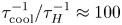
Despite the promising results of numerical simulations, there have been few experimental studies of radiatively cooled reconnection in the laboratory. The primary reason for this is the difficulty associated with achieving the plasma conditions required for observing radiative cooling effects on experimental time scales. As an example, table 1 summarizes the working conditions of some major reconnection experiments. We calculate the cooling time using an optically thin radiative loss model for simplicity, although more sophisticated radiation loss models which account for opacity and non-equilibrium emission can also be used for this calculation (Hare et al. Reference Hare, Suttle, Lebedev, Loureiro, Ciardi, Chittenden, Clayson, Eardley, Garcia and Halliday2018). For MRX (Ji et al. Reference Ji, Yamada, Hsu, Kulsrud, Carter and Zaharia1999; Yamada et al. Reference Yamada, Kulsrud and Ji2010) and laser-driven experiments (Fox, Bhattacharjee & Germaschewski Reference Fox, Bhattacharjee and Germaschewski2011, Reference Fox, Bhattacharjee and Germaschewski2012; Rosenberg et al. Reference Rosenberg, Li, Fox, Zylstra, Stoeckl, Séguin, Frenje and Petrasso2015), which have fully stripped ions, we use a recombination–bremsstrahlung model (Richardson Reference Richardson2019a), whereas, for the pulsed-power-driven experiments (Suttle et al. Reference Suttle, Hare, Lebedev, Swadling, Burdiak, Ciardi, Chittenden, Loureiro, Niasse and Suzuki-Vidal2016; Hare et al. Reference Hare, Suttle, Lebedev, Loureiro, Ciardi, Chittenden, Clayson, Eardley, Garcia and Halliday2018; Suttle et al. Reference Suttle, Hare, Lebedev, Ciardi, Loureiro, Burdiak, Chittenden, Clayson, Halliday and Niasse2018), we use emissivities calculated with the atomic code SpK, which includes line, bremsstrahlung and recombination emission (Crilly et al. Reference Crilly, Niasse, Fraser, Chapman, McLean, Rose and Chittenden2023). Inverse-Compton and cyclotron/synchrotron radiation mechanisms are not included, and are not expected to be significant. Of the experiments listed in table 1, pulsed-power-driven reconnection experiments exhibit the largest cooling parameter. Indeed, previous pulsed-power-driven experiments on 1 MA university-scale facilities have provided evidence for the onset of radiative cooling – Thompson scattering data show strong cooling of the ions in the reconnection layer (Hare et al. Reference Hare, Suttle, Lebedev, Loureiro, Ciardi, Chittenden, Clayson, Eardley, Garcia and Halliday2018; Suttle et al. Reference Suttle, Hare, Lebedev, Ciardi, Loureiro, Burdiak, Chittenden, Clayson, Halliday and Niasse2018). However, these pulsed-power-driven experiments conducted on 1 MA machines either achieve strong cooling at low (${<}10$ ) Lundquist numbers (Suttle et al. Reference Suttle, Hare, Lebedev, Swadling, Burdiak, Ciardi, Chittenden, Loureiro, Niasse and Suzuki-Vidal2016; Hare et al. Reference Hare, Suttle, Lebedev, Loureiro, Ciardi, Chittenden, Clayson, Eardley, Garcia and Halliday2018; Suttle et al. Reference Suttle, Hare, Lebedev, Ciardi, Loureiro, Burdiak, Chittenden, Clayson, Halliday and Niasse2018), or little cooling at relatively higher (${\sim }100$
 ) Lundquist numbers (Hare et al. Reference Hare, Lebedev, Suttle, Loureiro, Ciardi, Burdiak, Chittenden, Clayson, Eardley and Garcia2017a,Reference Hare, Suttle, Lebedev, Loureiro, Ciardi, Burdiak, Chittenden, Clayson, Garcia and Niasseb, Reference Hare, Suttle, Lebedev, Loureiro, Ciardi, Chittenden, Clayson, Eardley, Garcia and Halliday2018). In contrast, the pulsed-power experiments simulated here will simultaneously achieve both a higher Lundquist number and a high cooling parameter.
Table 1. Comparison of characteristic working conditions in laboratory experiments of magnetic reconnection, between MRX (Ji et al. Reference Ji, Yamada, Hsu, Kulsrud, Carter and Zaharia1999; Yamada et al. Reference Yamada, Kulsrud and Ji2010), laser-driven reconnection (Rosenberg et al. Reference Rosenberg, Li, Fox, Zylstra, Stoeckl, Séguin, Frenje and Petrasso2015), 1 MA pulsed power (Hare et al. Reference Hare, Suttle, Lebedev, Loureiro, Ciardi, Chittenden, Clayson, Eardley, Garcia and Halliday2018; Suttle et al. Reference Suttle, Hare, Lebedev, Ciardi, Loureiro, Burdiak, Chittenden, Clayson, Halliday and Niasse2018) and the MARZ experiments. Quantities above the horizontal line are reported values, while quantities below the line are calculated from the reported values using optically thin radiation models. For MRX and laser-driven experiments, which have fully stripped ions, we use a recombination–bremsstrahlung model (Richardson Reference Richardson2019a), whereas, for the pulsed-power-driven experiments, we use emissivities calculated with the atomic code SpK (Crilly et al. Reference Crilly, Niasse, Fraser, Chapman, McLean, Rose and Chittenden2023).
$^{a}$ Suttle et al. (Reference Suttle, Hare, Lebedev, Ciardi, Loureiro, Burdiak, Chittenden, Clayson, Halliday and Niasse2018) report a cooling time of 5 ns. However, using SpK as discussed below results in a shorter cooling time for relevant densities and temperatures.
The simulations presented in this paper were motivated by experiments run by the Magnetic Reconnection on Z (MARZ) collaboration, which uses the Z machine at Sandia National Laboratories to investigate radiatively cooled magnetic reconnection. The Z machine is a pulsed-power generator that delivers peak currents of $20\unicode{x2013}30\,{\rm MA}$ with $100\unicode{x2013}300\,{\rm ns}$
 rise times to a load inside a vacuum chamber (Sinars et al. Reference Sinars, Sweeney, Alexander, Ampleford, Ao, Apruzese, Aragon, Armstrong, Austin and Awe2020). For the MARZ experiments, we scale up the pulsed-power-driven magnetic reconnection platform developed on the MAGPIE generator at Imperial College London (Suttle et al. Reference Suttle, Hare, Lebedev, Swadling, Burdiak, Ciardi, Chittenden, Loureiro, Niasse and Suzuki-Vidal2016, Reference Suttle, Hare, Lebedev, Ciardi, Loureiro, Burdiak, Chittenden, Clayson, Halliday and Niasse2018; Hare et al. Reference Hare, Suttle, Lebedev, Loureiro, Ciardi, Chittenden, Clayson, Eardley, Garcia and Halliday2018), which consists of two inverse or ‘exploding’ cylindrical wire arrays, placed side by side and driven in parallel. Figure 1(a) shows a photograph of the load for the first MARZ experiment. Each array consists of 150 aluminium wires, $75\,\mathrm {\mu }{\rm m}$
 diameter arranged in a cylinder 40 mm in diameter around a thick central conductor.

Figure 1. (a) A photograph of the experimental load hardware for the MARZ experiments, which is the geometry we simulate using GORGON. Each array consists of 150 Al wires, $75\,\mathrm {\mu }{\rm m}$ diameter, evenly spaced in a cylinder 40 mm in diameter, 40 mm tall, with a centre-to-centre separation of 60 mm, or 20 mm between the wires of opposing arrays. (b) A three-dimensional model of the load hardware showing the direction of the current flow (purple), plasma ablation (red) and advected magnetic field (blue). The flows from each array interact in the mid-plane to form a current sheet. (c) The current pulse used in the Z experiments and the GORGON simulations, which is well approximated by $I = I_0 \sin ^2({\rm \pi} t/2\tau )$
 with $I_0 = 20\,{\rm MA}$
 and $\tau = 300\,{\rm ns}$
 .
.
The current from the generator passes through the wires and returns to ground through the central conductor, ohmically heating the wires until they undergo an ‘electrical explosion’, and form a heterogeneous liquid-droplet/vapour mixture. Further ohmic heating forms a coronal plasma around each wire, which is accelerated radially outwards by the $\boldsymbol {j}\times \boldsymbol {B}$ force due to the strong azimuthal magnetic field (${\approx }100$
 T) around the central conductor. As the plasma moves away from the wire, it advects with it some of this driving field, creating radially diverging supersonic super-Alfvénic outflows with frozen-in magnetic fields (Burdiak et al. Reference Burdiak, Lebedev, Bland, Clayson, Hare, Suttle, Suzuki-Vidal, Garcia, Chittenden and Bott-Suzuki2017; Suttle et al. Reference Suttle, Burdiak, Cheung, Clayson, Halliday, Hare, Rusli, Russell, Tubman and Ciardi2019; Datta et al. Reference Datta, Russell, Tang, Clayson, Suttle, Chittenden, Lebedev and Hare2022a,Reference Datta, Russell, Tang, Clayson, Suttle, Chittenden, Lebedev and Hareb). This process is referred to as ablation, and in the MARZ experiments, we choose an initial wire diameter such that the arrays are ‘over-massed’, and the wires act as stationary reservoirs of mass throughout the current pulse (Lebedev et al. Reference Lebedev, Beg, Bland, Chittenden, Dangor, Haines, Kwek, Pikuz and Shelkovenko2001; Harvey-Thompson et al. Reference Harvey-Thompson, Lebedev, Bland, Chittenden, Hall, Marocchino, Suzuki-Vidal, Bott, Palmer and Ning2009; Datta et al. Reference Datta, Angel, Greenly, Bland, Chittenden, Lavine, Potter, Robinson, Wong and Hammer2023).
When the radially accelerated plasma flows from the two wire arrays collide at the mid-plane, the advected magnetic fields are equal in magnitude and anti-parallel (see figure 1b). A current sheet forms at the mid-plane, and magnetic reconnection occurs. In these experiments, the plasma cools through a combination of bremsstrahlung, recombination, and line emission during the reconnection process. The cooling mechanisms in these laboratory experiments are therefore not the same as those in the extreme astrophysical plasmas discussed above, where synchrotron and other mechanisms are often more important. Although this is a limitation of these experiments, we are still qualitatively in the same regime, in which radiative cooling time scales are short enough to affect the dynamics of magnetic reconnection. As seen in table 1, pulsed-power-driven reconnection experiments achieve cooling parameters several orders of magnitude higher than other types of reconnection experiments.
In these experiments, the plasma flows are highly collisional (ion-ion collisional mean free path $\lambda _{ii} \sim 0.1-1\times 10^{-2}\,{\rm mm}$ ), and therefore, well approximated by magnetohydrodynamics (MHD) (Suttle et al. Reference Suttle, Burdiak, Cheung, Clayson, Halliday, Hare, Rusli, Russell, Tubman and Ciardi2019). The inflows to the reconnection layer are axially uniform, so any three-dimensional dynamics within the layer is the result of instabilities rather than the inflows. The driving current pulse is much longer than the Alfvén transit time so the inflows can be considered to be in approximate steady state, and rapid changes in the plasma dynamics are again the result of instabilities rather than the changing drive conditions. As we simulate the entire experimental domain from the start of the current pulse, we are inherently simulating a forming current sheet, rather than starting with an initial condition such as a Harris sheet.
In this paper, we present two-dimensional (2-D) and three-dimensional (3-D) MHD simulations of the MARZ experiments. To elucidate the effects of radiative cooling, we compare our 2-D results for the radiatively cooled and non-radiative cases, with a non-optically thin radiative loss model computed using the atomic code SpK (Crilly et al. Reference Crilly, Niasse, Fraser, Chapman, McLean, Rose and Chittenden2023). In both the non-radiative and radiatively cooled cases, the arrays generate magnetized supersonic (sonic Mach number $M_S = 4\unicode{x2013}5$ ), super-Alfvénic (Alfvén Mach number $M_A \approx 1.5$
 ) and super-fast magnetosonic (fast magnetosonic Mach number $M_{{\rm FMS}} \approx 1.4$
 ) flows which interact in the mid-plane to generate a current sheet. The current sheet exhibits a heterogeneous structure due to the presence of several fast-moving plasmoids. These plasmoids are sites of strong radiative emission due to their higher density and temperature compared with the rest of the layer, similar to observations in previous numerical studies of radiative reconnection (Schoeffler et al. Reference Schoeffler, Grismayer, Uzdensky, Fonseca and Silva2019; Sironi & Beloborodov Reference Sironi and Beloborodov2020; Schoeffler et al. Reference Schoeffler, Grismayer, Uzdensky and Silva2023). We find that radiative cooling modifies the reconnection process in several ways. First, it creates a denser, colder and thinner reconnection layer that exhibits strong compression, consistent with the theoretical prediction of Uzdensky & McKinney (Reference Uzdensky and McKinney2011). Second, the current sheet also becomes more uniform due to the cooling-driven extinction of plasmoids in the current sheet. Finally, there is also reduced flux pile up outside the layer, resulting in a lower magnetic field and density of the inflows into the sheet. The dynamics observed in the 2-D simulations is well reproduced in three dimensions. Furthermore, the plasmoids in the 3-D simulation also exhibit strong kinking along the axial direction. Radiation transport significantly modifies the inflow into the current sheet in both two dimensions and three dimensions, resulting in an initial lower driving magnetic pressure, which in turn, causes reduced compression of the layer after radiative collapse.
2. Simulation set-up
We perform compressible resistive-MHD simulations of a dual exploding wire array load using the code GORGON. GORGON is a 3-D (Cartesian, cylindrical or polar coordinates) Eulerian resistive-MHD code with van Leer advection (Chittenden et al. Reference Chittenden, Lebedev, Oliver, Yu and Cuneo2004b; Ciardi et al. Reference Ciardi, Lebedev, Frank, Blackman, Chittenden, Jennings, Ampleford, Bland, Bott and Rapley2007a). The simulation geometry consists of two exploding wire arrays with a centre-to-centre separation of $60\,{\rm mm}$ . Each array has a diameter of $40\,{\rm mm}$
 , and consists of 150 equally spaced $75\,\mathrm {\mu }{\rm m}$
 diameter aluminium wires. In three dimensions, the wires are 36 mm tall. The wire arrays are over-massed to provide continuous plasma ablation without exploding during the simulation. The initial mass in the wires is distributed over $3 \times 3$
 grid cells of pre-expanded wire cores. The current is applied to the wire array by setting the magnetic field in the region between the central conductor and the wires, using a current pulse of the form $I = I_0 \sin ^2({\rm \pi} t/2\tau )$
 with $I_0 = 20\,{\rm MA}$
 and $\tau = 300\,{\rm ns}$
 (figure 1c), chosen to simulate the Z machine's current pulse when operated in long-pulse mode (Sinars et al. Reference Sinars, Sweeney, Alexander, Ampleford, Ao, Apruzese, Aragon, Armstrong, Austin and Awe2020).
We first perform 2-D simulations in the $xy$ -plane (see figure 1b) on a $3200 \times 1760$
 Cartesian grid of dimensions $160 \times 88\,{\rm mm}^2$
 . The grid cell size is $\Delta x = 50\,\mathrm {\mu }{\rm m}$
 , which is adequate to resolve the resistive diffusion length $\bar {\eta }/V > 4 \Delta x$
 , calculated using the magnetic diffusivity $\bar {\eta }$
 of the reconnection layer, and the inflow velocity $V$
 . Two-fluid effects are not included in these simulations, and only the resistive-MHD equations are solved. Open boundary conditions are imposed on all sides of the computational domain. GORGON uses an adaptive time step, and we output the results of the simulation every 10 ns. The 2-D simulations were run for $2 \tau = 600\,{\rm ns}$
 , which is roughly $300$
 times the Alfvén crossing time $\delta /V_A$
 . Here, we have used averaged values of the Alfvén speed $V_A = B_{{\rm in}}/\sqrt {\mu _0 \rho _{{\rm in}}} \approx 50\,{\rm km}\,{\rm s}^{-1}$
 , calculated just outside the reconnection layer, and the reconnection layer half-width $\delta \approx 0.1\,{\rm mm}$
 at the time of peak current in the radiatively cooled simulation.
Three-dimensional simulations were also performed by extending the simulation domain by $36\,{\rm mm}$ (720 grid cells) in the $z$
 direction. The grid cell size is the same as that in the 2-D simulations. Reflective boundary conditions are used on the top and bottom surfaces of the simulation domain, while the sides of the simulation have open boundary conditions. The 3-D simulations, which are computationally more expensive, were run for $280\,{\rm ns}$
 , adequate to observe the formation and radiative collapse of the reconnection layer.
GORGON solves two coupled energy equations for the ions and electrons. Both the ions and electrons transport heat via thermal conduction, and are heated or cooled by compression or expansion. The ions are additionally heated by viscous heating, while the electrons are heated by ohmic dissipation. The ion and electron temperatures equilibrate at a collisional energy equilibration rate $\tau _{E}^{-1} = 3.2\times 10^{-9} n_i\bar {Z}^2 \ln \varLambda / (A T_e^{3/2})$ , where $\bar {Z}$
 is the ionization, $n_i$
 and $T_e$
 are the ion density and electron temperature, respectively, $\ln \varLambda$
 is the Coulomb logarithm and $A$
 is the ion mass in proton mass units (Ciardi et al. Reference Ciardi, Lebedev, Frank, Blackman, Chittenden, Jennings, Ampleford, Bland, Bott and Rapley2007b; Richardson Reference Richardson2019b). The equilibration time is initially of the order of the Alfvén transit time $\tau _A = L/V_A \sim 4 \tau _E$
 , but becomes much shorter later at times ($\tau _{E}/\tau _A \sim 10^{-4}$
 ), such that the ion and electron temperatures become equal. Here, we calculate the Alfvén transit time using the Alfvén speed in the inflow to the reconnection layer; $L$
 is the layer half-length $L \approx 18\,{\rm mm}$
 (see § 3.1 for details on how these quantities are calculated). We use a Thomas–Fermi equation of state to determine the (isotropic) pressure and ionization level of the plasma (Ciardi et al. Reference Ciardi, Lebedev, Frank, Blackman, Chittenden, Jennings, Ampleford, Bland, Bott and Rapley2007a). Transport coefficients are determined from Epperlein & Haines (Reference Epperlein and Haines1986), and vary spatially and temporally with changes in the plasma's electron temperature, density, average ionization and the magnitude and orientation of the magnetic field. The electrons also lose internal energy via radiative losses – accurate modelling of radiation is of particular importance in the description of the radiative collapse of the reconnection layer.
2.1. Radiation models
In the limit of negligible optical depth, radiation can be treated as an electron energy loss mechanism determined entirely by the plasma's total emissivity, $J$ . As optical depth increases, radiation transport effects become increasingly important as radiation emitted in one region can be reabsorbed in another. Using an optically thin radiation model in plasmas with finite opacity would result in an overestimation of the total energy loss from the system. However, solving radiation transport in large MHD simulations is a computationally intensive task. Therefore, to limit the total radiative loss compared with optically thin models, we explore a local loss model in our simulations, which is computationally less expensive than solving radiation transport. The effects of the local loss model are compared with $P_{1/3}$
 multi-group radiation transport.
In the local loss model, the optical depth of the computational cell itself is included in the calculation of the radiative power emitted by each individual cell. For an isotropically emitting spherical volume, an analytic solution for the radiative loss rate per unit volume, $P_{\text {rad}}$ , can be found from the time-independent frequency-resolved radiation transport equation (Crilly Reference Crilly2020)


where $R$ , $S$
, $S$ and $V$
 are the radius, surface area and volume of the sphere, $j_\nu$
 is the emissivity and $\kappa _\nu$
 is the absorption opacity. Scattering effects are not included in this model. For non-spherical volumes, such as the cubic computational cell used in these simulations, the radius is exchanged for the effective width of the cell as calculated by 3 times the volume-to-surface area ratio. As opposed to optically thin models, the optical depth of the computational cell limits the total radiative power lost from the cell. Radiation emitted by a given cell is, however, not re-absorbed by neighbouring cells in the local loss model, and lost from the system. While this approximation neglects re-absorption over length scales longer than a computational cell, and thus still over-estimates the total radiative loss, it serves as an improvement over optically thin models as energy is retained by the system due to local re-absorption which would have otherwise been lost.
Numerically, a multi-group approach can be used to evaluate the local loss model for $P_{\text {rad}}$ using opacities and emissivities from tables. In GORGON, multi-group tables from the code SpK are used (Crilly et al. Reference Crilly, Niasse, Fraser, Chapman, McLean, Rose and Chittenden2023). SpK performs detailed configuration accounting calculations of electronic and ionic stage populations in either local thermal equilibrium (LTE) or non-local thermodynamic equilibrium (NLTE) through an effective temperature approach. The radiation model includes free–free, free–bound and bound–bound transitions from which opacities and emissivities are calculated, which are functions of the local ion density and electron temperature.
Local loss models provide sufficient accuracy to perform design calculations and investigate the physical phenomena for the radiatively cooled reconnection platform. Figure 2 shows results of the local loss model (2.1) for an aluminium plasma. It is clear from figure 2(a) that an NLTE description is required to accurately calculate the radiative power at lower densities. The simulations in this paper, therefore, use NLTE opacity and emissivity tables from SpK, which are valid for the range in density and temperature accessible to the MARZ experiments. We note that a corresponding NLTE effect on the equation of state will exist but the corrections are considerably smaller than on the radiative power. It is also shown in figure 2(b) that L-shell line emission is dominant at temperatures around 100 eV, thus continuum loss models which only include bremsstrahlung and radiative recombination are inaccurate. Additionally, the local loss model predicts large corrections to the radiative loss in denser plasma due to optical depth effects, as seen in figure 2(c).

Figure 2. (a) The optically thin ($\tau = 0$ ) radiative power of Al plasma at an electron density of $1\times 10^{17}\,{\rm cm}^{-3}$
 and varied temperature calculated by SpK in LTE and NLTE. (b) The optically thin radiative power at various electron densities and temperatures. Results from NLTE SpK with and without bound–bound (BB) transitions are compared with NLTE FLY tables (Chung, Morgan & Lee Reference Chung, Morgan and Lee2003; Chung et al. Reference Chung, Chen, Morgan, Ralchenko and Lee2005). (c) SpK predictions of the local loss radiative power for a $R = 50\,\mathrm {\mu }{\rm m}$
 sphere as a function of temperature.
For a more accurate description of the experiment, a limited number of 2-D and 3-D simulations were also run with $P_{1/3}$ multi-group radiation transport, the numerical implementation of which can be found in Crilly et al. (Reference Crilly, Niasse, Fraser, Chapman, McLean, Rose and Chittenden2023). In the $P_{1/3}$
 multi-group radiation transport model, radiation emitted by a given cell can be absorbed and re-emitted by plasma in other parts of the simulation domain. This task, however, is computationally more expensive than the local loss model described above. We discuss the importance of radiation transport modelling in § 3.3.
3. Two-dimensional simulations
3.1. Results
We describe and compare the 2-D ($xy$ -plane) simulation results for two cases, first for the non-radiative case in which we artificially turn off all radiative losses from the plasma, and next for the radiatively cooled case where the losses are implemented using the local loss radiation model described above.
3.1.1. Non-radiative case
Figure 3(a) shows the electron density distribution at $t = 200$ ns after the start of the current pulse for the case with no radiative emission. Each wire array generates radially diverging plasma flows, so the electron density is high close to the wires and decreases with distance from the arrays. The electron density from each array also exhibits a periodic small-scale modulation in the azimuthal direction, due to the supersonic collision of adjacent azimuthally expanding ablation flows from the individual wire cores (Swadling et al. Reference Swadling, Lebedev, Niasse, Chittenden, Hall, Suzuki-Vidal, Burdiak, Harvey-Thompson, Bland and De Grouchy2013). This results in the formation of standing oblique shocks, periodically distributed in the azimuthal direction. The length scale of this azimuthal modulation is comparable to the inter-wire separation of around $0.8\,{\rm mm}$
 .
.

Figure 3. (a) Electron density at 200 ns after current start from 2-D resistive-MHD simulations for the non-radiative case. The wire arrays generate radially diverging flows which interact at the mid-plane to generate a current sheet. (b) Electron density at 200 ns after current start for the radiatively cooled case. (c–e) Electron density in the reconnection layer at 150, 200 and 300 ns after current start for the non-radiative case showing the formation of plasmoids. (f) Current density and superimposed magnetic field lines in the reconnection layer at 300 ns after current start for the non-radiative case showing flux pile up and plasmoids. (g–i) Electron density in the reconnection layer at 150, 200 and 300 ns after current start for the radiatively cooled case. (f) Current density and superimposed magnetic field lines in the reconnection layer at 300 ns after current start for the radiatively cooled case.
The plasma flows advect magnetic field from the inside of the array as they propagate radially outwards. The magnetic field lines are oriented azimuthally with respect to the centre of each array. The plasma flows with oppositely directed and symmetrically driven magnetic fields interact at the mid-plane ($x = 0$ ) to generate a current sheet. The structure and time evolution of the current sheet are shown in figure 3(c–f). The current sheet appears as an elongated region of enhanced current (see figure 3f) and electron density at the mid-plane. Magnetic field lines oriented in the $\pm y$
 -direction are driven into the current sheet by the inflows, and exit the reconnection layer as curved reconnected field lines, as seen in figure 3(f). The current sheet first forms at $t \approx 100\,{\rm ns}$
 , consistent with the transit time between the wire locations and the mid-plane, and a flow velocity of $100\,{\rm km}\,{\rm s}^{-1}$
 (Hare et al. Reference Hare, Lebedev, Suttle, Loureiro, Ciardi, Burdiak, Chittenden, Clayson, Eardley and Garcia2017a; Suttle et al. Reference Suttle, Hare, Lebedev, Ciardi, Loureiro, Burdiak, Chittenden, Clayson, Halliday and Niasse2018). The current and electron density in the sheet increase with time. This is due to increased ablation from the wires as the magnitude of the driving current ramps up over time.
Figure 4 shows the temporal evolution of the length $2L$ and width $2 \delta$
 of the current sheet. We define $2L$
 as the full width at half-maximum (FWHM) of the out-of-plane current density $j_z$
 in the $y$
 -direction. To calculate the length of the current sheet, we first integrate $j_z$
 in the $x$
 -direction in the range $-1\,{\rm mm} \leq x \leq 1\,{\rm mm}$
 , then compute the FWHM of a Gaussian fit to the line-integrated current density. Similarly, to calculate the sheet width, we first integrate $j_z$
 in $y$
 in the range $-L \leq y \leq L$
 . We define the sheet width $2\delta$
 based on a Harris sheet profile $[B_y(x) = \tanh (x/\delta ); j_z = {\rm sech}^2(x/\delta )/\delta ]$
 . For a Harris sheet, $j_z$
 falls to 10 % of its peak value at $x=x_{10}=\pm 1.82\delta$
 , so $\delta$
 can be calculated as $\delta \approx x_{10}/1.82$
 . For Harris-like current sheets, $\delta$
 estimated via the aforementioned method will be consistent with that approximated from the FWHM of $j_z$
 , i.e. $2\delta \approx \text {FWHM}/ 0.9$
 . In our simulations, $j_z$
 appears Harris-like for the non-radiative case, but becomes flat topped for the radiatively cooled case. Using the FWHM to estimate $\delta$
 in the radiatively cooled case results in an overestimate of the sheet width, while using $\delta \approx x_{10}/1.82$
 provides results that more appropriately capture the current sheet width. We use $10\,\%$
 of the peak $j_z$
 for this calculation in order to capture most of the current distribution.

Figure 4. Variation of current sheet length (a) and current sheet width (b) with time for the non-radiative and radiatively cooled cases.
For the non-radiative case (black circles in figure 4), the sheet length initially increases rapidly with time ($t < 200\,{\rm ns}$ ), and then continues to rise at a much slower rate. After the early transient period, the value of $2L \approx 35\,{\rm mm}$
 is comparable to the radius of curvature of the field lines at the current sheet. The width of the current sheet also exhibits an increase with time; the increase in $2\delta$
 is modest, and the sheet width remains in the range $0.4\,{\rm mm} \leq 2\delta \leq 0.6\,{\rm mm}$
 during $150\unicode{x2013}350\,{\rm ns}$
 . The aspect ratio of the sheet after the formation stage is thus $\delta /L \approx 0.01$
 . Both $2L$
 and $2\delta$
 also increase faster later in time ($t \geq 350\,{\rm ns}$
 ). This is related to a change in the ablation conditions due to explosion of the wire array, as the wires begin to run out of mass at this late time. In this paper, however, we are interested in the reconnection dynamics well before this late time.
The current sheet exhibits a non-uniform structure, with elliptical islands of higher electron density separated by thin elongated regions. These density concentrations correspond to the locations of magnetic islands or ‘plasmoids.’ This can be observed in figure 3(f), which illustrates the distribution of current density $j_z$ with superimposed magnetic field lines. The presence of plasmoids is consistent with magnetic reconnection at the current sheet, and indicates that the current sheet is unstable to the plasmoid instability (Loureiro, Schekochihin & Cowley Reference Loureiro, Schekochihin and Cowley2007). The plasmoids envelop magnetic O-points in the reconnection layer, and are separated by individual X-points. More discussion on the structure and temporal evolution of the plasmoids is provided in § 3.2.4.
Figure 3(c–f) also shows the presence of shocks upstream of the current sheet. Each shock appears as a discontinuous enhancement of the electron density in figure 3(c–e), and a thin region of negative current density in figure 3(f). The presence of the shocks upstream of the current sheet is consistent with magnetic flux pile up in a compressible system with super-magnetosonic inflows. Magnetic flux pile up is expected to occur when the flux injection rate exceeds the flux annihilation rate in the reconnection layer (Biskamp Reference Biskamp1986). We discuss flux pile up in more detail in § 3.2.1.
Figure 5(a–d) shows the lineouts of ion density $n_i$ , the $y$
 -component of the magnetic field $B_y$
 , the $x$
 -component of the velocity field $V_x$
 and the electron temperature $T_e$
 . The lineouts are taken along the $x$
 -axis, and each quantity is line averaged in the $y$
 -direction in the range $-L/2 < y < L/2$
 . As shown in figure 5(b), magnetic flux pile up divides the plasma into 4 distinct regions – (A) an inflow region upstream of the shock, (B) the shock transition region, (C) a post-shock region and, finally, (D) the reconnection layer.

Figure 5. Lineouts of ion density, magnetic field ($y$ -component), flow velocity ($x$
 -component) and electron temperature as a function of $x$
 for the non-radiative case (a–d), and the radiatively cooled case (e–h). In the non-radiative case, we see significant flux pile up outside the layer, which leads to a ${\approx }2 \times$
 compression of the magnetic field and density in the inflows to the reconnection layer. In the radiatively cooled case, we observe reduced flux pile up and strong compression and cooling of the current sheet.
Consistent with time-of-flight effects and radially diverging flow, the ion density and the magnetic field strength fall with increasing distance from the wires in the inflow region. The shock results in compression of both the ion density and the magnetic field by a factor of approximately $2$ , while the velocity exhibits a sharp downward jump at the shock front. The sharp gradient in the magnetic field at the shock is consistent with the negative current density $\mu _0 j_z = \partial _x B_y - \partial _y B_x$
 observed in figure 3(f), as expected from Ampere's law. The temperature also increases at the shock front due to compressional heating. The shocks propagate upstream with a velocity of approximately $10\,{\rm km}\,{\rm s}^{-1}$
 , around $10\,\%$
 of the inflow velocity.
The magnetic field continues to exhibit a gradual pile up in the post-shock region, while the density decreases behind the propagating shock wave. As expected, the $y$ -component of the magnetic field and the $x$
 -component of velocity undergo a reversal in direction inside the reconnection layer. The magnetic field $B_y$
 and the inflow velocity $V_x$
 approach 0 at the centre of the reconnection layer ($x = 0\,{\rm mm}$
 ). The mass density inside the reconnection layer is similar to that just outside of the layer, indicating weak compression, while the electron temperature at the centre of the layer is significantly higher ($T_e \approx 100\,{\rm eV}$
 ) than that just outside the layer ($T_e \approx 10\,{\rm eV}$
 ). This is consistent with the ohmic dissipation of magnetic energy into internal energy during reconnection. Because of the temporal change in the driving current, the ion density and magnetic field increase with time, consistent with increased ablation from the wire arrays. The electron temperature, however, remains roughly constant with a value of $T_e \approx 10\,{\rm eV}$
 in the inflow, and $T_e \approx 100\,{\rm eV}$
 in the reconnection layer.
3.1.2. Radiatively cooled case
Figure 3(b) shows the electron density distribution from the wire arrays at $t = 200\,{\rm ns}$ for the radiatively cooled case. Similarly, figure 3(g–j) shows the electron density and current distribution in the reconnection layer for the radiatively cooled case. The plasma outflows from the arrays, which are inflows into the reconnection layer, appear qualitatively similar to the non-radiative case. Early in time ($t < 200\,{\rm ns}$
 ), the structure of the current sheet, and that of the upstream shock, are also similar to those in the non-radiative case. Lineouts along the $x$
 -axis (figure 5e–g) shows that the magnitudes of the line-averaged ion density, magnetic field $B_y$
 and inflow velocity $V_x$
 in the inflow region far from the current sheet remain almost identical to the non-radiative case. The electron temperature in the inflow is also similar to the non-radiative case early in time ($t = 150\,{\rm ns}$
 ). However, as a consequence of radiative cooling, $T_e$
 in the inflow (2.5 eV at 400 ns) becomes lower than the non-radiative inflow temperature (8 eV at 400 ns) later in time (figure 5h).
The structure of the current sheet exhibits significant differences after $t \geq 200\,{\rm ns}$ . Figure 3(h–j) shows a much thinner and denser current sheet than in the non-radiative case. In figure 4(b), we compare the length $2L$
 and width $2\delta$
 of the current sheet with that for the non-radiative case. Initially, the dimensions of the current sheet in both cases are almost identical. For $t \geq 200\,{\rm ns}$
 , however, the radiatively cooled current sheet becomes much thinner than in the non-radiative case, whereas the length remains approximately equal in the two cases. This results in a significantly smaller aspect ratio $\delta /L$
 in the radiatively cooled case. Moreover, whereas in the non-radiative case, we observe a modest increase in layer width over time, in the radiatively cooled case, $2\delta$
 is remarkably mostly constant within the interval $220\,{\rm ns} \leq t \leq 350\,{\rm ns}$
 (figure 4).
The higher density and smaller width of the current sheet indicate strong compression of the current sheet due to radiative cooling. This can also be observed in lineouts of the ion density along the $x$ -axis (figure 5e), which show significantly higher density in the reconnection layer after $t = 200\,{\rm ns}$
 . The strong compression in the layer is indicative of radiative collapse. Evidence of radiative collapse is also observed from the significant decrease in the temperature in the layer (figure 5h), which falls from $T_e \approx 100\,{\rm eV}$
 initially to $T_e \approx 10\,{\rm eV}$
 at $t = 400\,{\rm ns}$
 after current start. In contrast, in the non-radiative case, the electron temperature remains high around $T_e \approx 100\,{\rm eV}$
 throughout the simulation (figure 5d), which is much higher than in the radiatively cooled case. We will discuss this increase in density and drop in temperature in the context of the overall pressure balance of the layer in § 3.2.3. Finally, we can observe plasmoids in the current sheet at $t = 200\,{\rm ns}$
 (figure 3h); however, these plasmoids disappear later in time, as seen in figure 3(i), creating a relatively homogeneous reconnection layer.
Radiative cooling also modifies magnetic flux pile up outside the reconnection layer. Early in time, we still observe shocks upstream of the current sheet (figure 3h). However, for $t > 200\,{\rm ns}$ , pile up is no longer mediated by a shock, as observed in figure 5(e–h). Instead, there is a relatively small accumulation of magnetic flux just outside the reconnection layer (figure 5f), while the ion density remains continuous, and only undergoes compression inside the reconnection layer. Consequently, the properties of the plasma just outside the current sheet are different compared with the non-radiative case.
The primary effects of radiative cooling on the structure of the reconnection layer can be summarized as follows: (i) radiative cooling leads to a denser and thinner current sheet, indicating strong density compression; (ii) the current sheet is significantly colder than in the non-radiative case; (iii) the current sheet is more uniform; plasmoids that are observable initially disappear later in time; and (iv) there is reduced flux pile up outside the layer, resulting in lower magnetic field and density just outside the layer, than in the non-radiative case. We provide further discussion on these effects in the next section.
3.2. Discussion of two-dimensional simulations
In this section, we compare and contrast the simulation results from the non-radiative and radiatively cooled cases. In § 3.2.1, we discuss the decreased magnetic flux pile up outside the layer observed in the radiatively cooled case, which results in a lower magnetic field and density of the inflow into the current sheet. Next, we discuss the global properties of the layer in § 3.2.2, and characterize differences in outflows from the reconnection layer, and in the global reconnection rate. We then discuss the radiatively driven strong compression of the current sheet, which generates a thinner and denser layer in the radiatively cooled simulation (§ 3.2.3). Finally, we discuss the differences in plasmoid structure and temporal evolution between the two cases in § 3.2.4. In the non-radiative case, plasmoids continue to grow after formation, while they collapse in the radiatively cooled case, generating a comparatively homogenous current sheet.
3.2.1. Magnetic flux pile up
In the non-radiative case, and in the radiatively cooled case before the onset of collapse, we observe the formation of shocks on either side of the reconnection layer due to magnetic flux pile up. Flux pile up occurs when the rate of magnetic flux injection $\tau _\text {inj}^{-1}/\tau _A^{-1} \sim V_\text {in}/V_{A,1} \equiv M_{A,1}$ exceeds that of flux annihilation in the reconnection layer $\tau _R^{-1}/\tau _A^{-1}$
 (Biskamp Reference Biskamp1986). Here, $\tau _{\text {inj}}^{-1}$
 and $\tau _R^{-1}$
 are the flux injection and reconnection rates respectively, $\tau _A$
 is the Alfvén transit time, $V_{\text {in}}$
 is the inflow velocity and $V_{A,1}$
 and $M_{A,1}$
 are the Alfvén velocity and Mach number in the inflow, respectively. Magnetic flux accumulates outside the current sheet, resulting in a local enhancement of the inflow magnetic field and a decrease in the inflow velocity, such that the injection rate is reduced until it matches the flux annihilation rate. In incompressible sub-Alfvénic flows which satisfy the pile-up condition $M_{A,1} > \tau _R^{-1}/\tau _A^{-1}$
 , pile up is gradual and continuous (Biskamp Reference Biskamp1986). However, in cases where the inflows are super-fast magnetosonic, flux pile up is abrupt, and mediated by a shock upstream of the reconnection layer. The presence of shock-mediated pile up has previously been observed in experimental studies of reconnection with high Mach number flows (Fox et al. Reference Fox, Bhattacharjee and Germaschewski2011; Suttle et al. Reference Suttle, Hare, Lebedev, Ciardi, Loureiro, Burdiak, Chittenden, Clayson, Halliday and Niasse2018; Olson et al. Reference Olson, Egedal, Clark, Endrizzi, Greess, Millet-Ayala, Myers, Peterson, Wallace and Forest2021).
To estimate the jumps in density and magnetic field across the shock, we calculate the sonic $M_S = U_1/C_S,$ Alfvénic $M_A = U_1/V_A$
 and fast magnetosonic $M_{{\rm FMS}} = U_1/(V_A^2 + C_S^2)^{1/2}$
 Mach numbers just upstream of the shock. Here, we calculate the sonic and Alfvén speeds using $C_S = \sqrt {\gamma p / \rho }$
 and $V_A = B / \sqrt {\mu _0 \rho }$
 , respectively, where $p$
 is the thermal pressure, $\rho$
 is the mass density, $\gamma = 5/3$
 is the adiabatic index, $U_{1}$
 is the flow velocity in the shock reference frame and $B$
 is the magnetic field strength just upstream of the shock. We use line-averaged values integrated in the $y$
 -direction in the range $|y| < L /2$
 for this calculation. The outflows from the wire arrays (for the non-radiative case) are supersonic ($M_S = 4.6 \pm 0.5$
 ), super-Alfvénic ($M_A = 1.5 \pm 0.1$
 ) and super-fast magnetosonic ($M_{{\rm FMS}}\approx 1.4 \pm 0.1$
 ). The Mach numbers remain relatively constant in time, despite the changing density, magnetic field and velocity of the upstream flow. The compression ratios of the line-averaged density and magnetic field across the shock, also remain relatively constant in time, as expected from the unchanging upstream Mach numbers. In the simulation, both the mass density and the magnetic field are compressed by a similar magnitude across the shock, exhibiting a compression ratio of $1.8 \pm 0.4$
 , consistent with ideal-MHD compression.
We can model the shock transition as a fast perpendicular MHD shock, which represents a super-fast to sub-fast transition in a system with an upstream magnetic field perpendicular to the shock normal. Solutions to the Rankine–Hugoniot jump conditions show that both the upstream magnetic field and mass density are compressed by the same ratio $r$ , which can be determined from the solution of a quadratic equation (Goedbloed, Keppens & Poedts Reference Goedbloed, Keppens and Poedts2010)

Here, $M_S$ is the upstream sonic Mach number, and $\beta$
 is the upstream plasma beta. The predicted compression ratio from (3.1), using $M_S = 4.6 \pm 0.5$
 and $\beta = 0.12 \pm 0.05$
 , is $r = 1.5 \pm 0.4$
 , which is consistent with the range observed in the simulation. The predicted compression ratio is slightly lower than the mean compression observed in the simulation, and may result from our assumption of a planar 1-D shock which neglects the velocity component parallel to the shock caused by the radial outflows from the wire arrays. As a consequence of the flux pile up, the downstream Alfvén Mach number, and consequently the flux injection rate into the reconnection layer, are both reduced by a factor of $r^{-3/2}$
 .
.
Results from the radiatively cooled simulation show decreased flux pile up compared with the non-radiative case after the onset of radiative collapse. This is consistent with the increase in the reconnection rate due to the strong compression of the current sheet observed in the radiatively cooled case. We expect the flux annihilation rate to be enhanced by a factor of $A^{1/2}$ in the radiatively cooled reconnection system (Uzdensky & McKinney Reference Uzdensky and McKinney2011). Here, $A \equiv \rho _{\text {layer}}/\rho _{\text {in}}$
 is the ratio of the mass density of the reconnection layer to that just outside the layer. Because of the increased reconnection rate, a higher flux injection rate can be supported, reducing flux pile up. A more detailed discussion of the effect of radiative cooling on the reconnection rate is provided in the next subsection. Flux pile up modifies the plasma conditions just outside the reconnection layer, and thus must be accounted for in the analysis of experimental data before the onset of radiative collapse, or even after collapse in cases where the compression of the layer is weak enough that the flux injection rate exceeds the reconnection rate, as described later in § 3.3.
3.2.2. Lundquist number, outflow velocity and reconnection rate
Figure 6(a) compares the temporal evolution in the Lundquist number $S_L = V_{{A,\text {in}}}L/\bar {\eta }$ for the non-radiative and radiatively cooled cases. Here, $V_{{A,\text {in}}}$
 is the Alfvén speed calculated just outside the current sheet at $x = \pm 2\delta$
 , and $\bar {\eta }$
 is the magnetic diffusivity of the layer, averaged over the current sheet between $|x| \leq \delta$
 . In the non-radiative case, the Lundquist number $S_L$
 increases as the current sheet forms, then reaches a relatively stationary value of $S_L \approx 400$
 at $t \geq 170\,{\rm ns}$
 . For the radiatively cooled case, the Lundquist number is similar to that in the non-radiative case early in time, but begins to fall at $t \approx 150\,{\rm ns}$
 , and reaches a steady value of $S_L \approx 100$
 later in time ($t \geq 200\,{\rm ns}$
 ). The change in the Lundquist number is consistent with the time of onset of radiative cooling, as observed in § 3.1.2. The lower Lundquist number in the radiatively cooled case is primarily a consequence of reduced layer temperature (figure 5h). As mentioned in § 3.1.2, the layer temperature falls from approximately 100 eV to 10 eV due to radiative cooling. Since the plasma (Spitzer) resistivity scales with electron temperature as $\eta \sim \bar {Z}T^{-3/2}$
 , a lower temperature leads to a more resistive layer, and the global Lundquist number $S_L$
 becomes smaller. The average ionization $\bar {Z}$
 in the current sheet also changes from approximately $11$
 in the non-radiative case, to approximately $3.5$
 in the radiatively cooled case, but this does not compensate for the change in temperature.

Figure 6. (a) Time evolution of the Lundquist number the non-radiative (black) and the radiatively cooled cases (red). The Lundquist number is lower for the radiatively cooled case. (b) Time evolution of the density compression ratio of the current sheet for the non-radiative (black) and the radiatively cooled cases (red). Results are shown for $t \geq 150\,{\rm ns}$ , before which the layer has not fully formed.
In figure 6(b), we compare the density compression ratios $A \equiv \rho _{\text {layer}}/\rho _{\text {in}}$ of the current sheet for the non-radiative and radiatively cooled cases. For the non-radiative case, the mass densities inside and outside the layer are similar, resulting in a compression ratio of $A \approx 1$
 . The compression ratio for the radiatively cooled case is also approximately 1 early in time, but as radiative losses from the layer become more significant, the compression ratio begins to increase around 170 ns, and approaches $A \approx 13$
 later in time. The strong compression of the current sheet due to radiative cooling is indicative of radiative collapse. This occurs when an increase in compression of the layer causes radiative losses to increase faster than ohmic dissipation (Uzdensky & McKinney Reference Uzdensky and McKinney2011). We revisit radiative collapse of the layer in § 3.2.3.
In the non-radiative case, the ion sound speed inside the layer $C_{S,CS}$ is comparable to the Alfvén speed in the inflow $V_{{A,\text {in}}}$
 , which indicates that the magnetic tension and pressure gradient forces are roughly equal in magnitude. The outflow velocity is higher than the inflow Alfvén velocity $V_{{A,\text {in}}}$
 and is comparable to the magnetosonic velocity (calculated from the combination of the sound and Alfvén speeds $V_{MS}^2 \equiv V_{{A,\text {in}}}^2 + C_{S, CS}^{2}$
 ). Here, we calculate the outflow velocity at a distance $y = L$
 from the centre of the layer, averaged over $-\delta \leq x \leq \delta$
 across the layer. This shows that both magnetic tension and the pressure gradient force play a role in accelerating the plasma in the reconnection layer. This effect has been observed previously in simulations (Forbes & Malherbe Reference Forbes and Malherbe1991), in pulsed-power-driven experiments of carbon wire arrays (Hare et al. Reference Hare, Lebedev, Suttle, Loureiro, Ciardi, Burdiak, Chittenden, Clayson, Eardley and Garcia2017a) and in MRX experiments where the thermal pressure upstream of the outflow region decelerates the outflows (Ji et al. Reference Ji, Yamada, Hsu, Kulsrud, Carter and Zaharia1999).
In the radiatively cooled case after radiative collapse, the sound speed in the layer $C_{S,CS}$ is lower than the inflow Alfvén speed $V_{{A,\text {in}}}$
 by a factor of ${>}2$
 , consistent with the decreased layer temperature. The magnetosonic velocity is then approximately equal to the Alfvén speed $V_{MS} \approx V_{{A,\text {in}}}$
 , and the outflow velocity, therefore, agrees well with the Alfvén velocity in the inflow. The plasma is primarily accelerated by the magnetic tension of the reconnected field. Consequently, the outflow velocity is smaller in the radiatively cooled case than in the non-radiative case, where the plasma is accelerated by both magnetic tension and pressure gradient forces. This is consistent with Uzdensky & McKinney (Reference Uzdensky and McKinney2011), which shows that, unlike in usual Sweet–Parker theory, the tension force is expected to be much larger than the pressure gradient force in the radiatively cooled case.
In figure 7, we compare the normalized reconnection rate $\tau _R^{-1}/\tau _H^{-1}$ between the two cases. Here, $\tau _R \equiv L/V_{\text {{in}}}$
 is the reconnection time determined from the flow velocity into the layer $V_{\text {in}}$
 at $x = \pm 2 \delta$
 , and $\tau _H \equiv L/V_{\text {out}}$
 is the hydrodynamic time calculated using the outflow velocity from the reconnection layer. After layer formation, the reconnection rate assumes a steady value of $\tau _R^{-1}/\tau _H^{-1} = V_{\text {in}}/V_{\text {out}} \approx 0.1$
 for the non-radiative case. In the radiatively cooled case, the reconnection rate increases from an initial value of about $0.1$
 and reaches a value of roughly 0.9, approximately $9$
 times higher than the non-radiative rate. For both cases, the reconnection rate is consistent with the scaling provided by compressible Sweet–Parker theory with radiative cooling, i.e. $V_{\text {in}}/V_{\text {out}} \sim A^{1/2}S_L^{-1/2}$
 (Uzdensky & McKinney Reference Uzdensky and McKinney2011). In figure 7, we use a constant of proportionality = $2.5$
 . We can attribute the high reconnection rate in the radiatively cooled case to strong compression of the current sheet ($A \approx 13$
 ), and to the lower Lundquist number $S_L \approx 100$
 of the colder layer.

Figure 7. Reconnection rate for the non-radiative (a), and radiatively cooled cases (b). Here, a factor of 2.5 is used as the constant of proportionality for the theoretical scaling. Results are shown for $t \geq 150\,{\rm ns}$ , before which the layer has not fully formed.
3.2.3. Radiative collapse
The radiative collapse of the reconnection layer is characterized by a sharp decrease in its temperature, and strong compression of the layer. To understand the temporal evolution of the layer temperature, we probe the various terms in the energy equation. In our system, ohmic and compressional heating are the dominant sources of internal energy addition to the layer, while radiative loss is the dominant loss term. Contributions of the advective terms, viscous heating, and conductive losses are comparatively small. In figure 8(a), we compare the volumetric radiative power loss $P_{{\rm rad}}$ , ohmic dissipation rate $P_\varOmega = \eta j^2$
 and the compressional heating rate $P_{{\rm comp.}} =-p(\boldsymbol {\nabla } \boldsymbol {\cdot } \boldsymbol {v})$
 in the current sheet. The radiative loss from the layer is around $2$
 times larger than the total heating provided by the ohmic and compressional terms. Radiative losses are initially smaller than ohmic dissipation right after layer formation, but begin to dominate at $t \approx 200\,{\rm ns}$
 , which is consistent with the sharp drop in the electron temperature and simultaneous density compression of the current sheet at this time, as shown in figure 8(b). We quantify the relative importance of radiative loss using the cooling parameter $R_{\text {cool}} \equiv \tau _{\text {cool}}^{-1}/\tau _{A}^{-1}$
 , which is the ratio of the radiative cooling rate $\tau _{\text {cool}}^{-1} = (\gamma -1) P_{\text {rad}}/p_{\text {th}}$
 to the Alfvénic transit rate $\tau _{A}^{-1} = V_{{A,\text {in}}}/L$
 in the layer, as mentioned earlier in § 1.1. Figure 8(c) shows that the cooling parameter is small initially, but rises sharply in the range $180 < t < 200\,{\rm ns}$
 to reach a value of $R_{\text {cool}} \approx 100$
 . The rise in the cooling parameter is consistent with the time at which we observe radiative cooling to become significant in § 3.1.2.

Figure 8. (a) Radiative loss and ohmic dissipation in the radiatively cooled current sheet. (b) Temporal evolution of current sheet mass density and electron temperature. (c) Variation of the cooling parameter with time. (d) Pressure balance in the current sheet. Results are shown for $t \geq 150\,{\rm ns}$ , before which the layer has not fully formed.
Finally, we compare the thermal pressure inside the current sheet $p_{\text {th}}$ with the kinetic $\rho _{\text {in}}V_{\text {in}}^2/2$
 and magnetic pressures $B_{\text {in}}^2/2\mu _0$
 upstream of the layer (figure 8d). The thermal pressure roughly balances the combined upstream kinetic and magnetic pressures. The thermal pressure in the layer continues to rise despite the sharp fall in the layer electron temperature. This is facilitated by the simultaneous increase in the density of the layer, as seen in figure 8(b). Compression of the layer, therefore, maintains pressure balance with the upstream kinetic and magnetic pressures.
3.2.4. Plasmoid behaviour
In the previous section, we looked at the global properties of the layer by taking 1-D profiles, averaged along the length of the layer. However, by taking these averages, we overlook the significant modulations in the plasma properties along the $y$ -direction caused by the plasmoids. Here, we look at the plasmoids in detail, and in particular we characterize the temporal evolution of the widths of the plasmoids.
Figure 9 shows the reconnection layer at $t=200\,{\rm ns}$ after current start, with plasmoids in both the radiatively cooled and non-radiative cases. We choose this time as it is after the onset of radiative cooling, but before the disappearance of the plasmoids in the radiatively cooled simulation. The findings at this time are also generally representative of later times in the non-radiative simulation. We observe plasmoids at Lundquist numbers of 200–400, which is lower than the canonical critical Lundquist number of $S_{L,C} \sim 10^4$
 (Loureiro et al. Reference Loureiro, Schekochihin and Cowley2007). The presence of plasmoids at these Lundquist numbers, however, is consistent with observations of plasmoids at $S_L \sim 100$
 in previous pulsed-power-driven experiments (Hare et al. Reference Hare, Suttle, Lebedev, Loureiro, Ciardi, Burdiak, Chittenden, Clayson, Garcia and Niasse2017b). Modulation in the inflows caused by the discrete nature of the wires may seed this instability, enabling it to occur at $S_L < S_C$
 . Furthermore, the system is highly compressible, strongly driven and exhibits non-uniform resistivity, which are effects not included in the original calculation of the critical Lundquist number.

Figure 9. (a–c) For the non-radiative case; 2-D maps of (a) current density $j_z$ overlaid by contours of the magnetic vector potential $A_z$
 , (b) electron temperature $T_e$
 , (c) electron density $n_e$
 . (d–g) For the radiatively cooled case; 2-D maps of (d) current density $j_z$
 overlaid by contours of the magnetic vector potential $A_z$
 , (e) electron temperature $T_e$
 , (f) electron density $n_e$
 . (g) Radiative power loss per unit volume, as generated by XP2 (see § 5).
For the non-radiative case (figure 9a), we plot the current density $j_z$ overlaid with the contours of the magnetic vector potential $A_z$
 (which are the magnetic field lines), and we show the electron temperature $T_e$
 and density $n_e$
 in figure 9(b,c). In this case, we see that the plasmoids (O-points in $A_z$
 ) carry more current than the current sheets or layers (X-points in $A_z$
 ) which separate them; the current density in the plasmoids is higher than in the sheets by a factor of approximately 2. Additionally, we observe that the plasmoids are significantly hotter than the rest of the reconnection layer (by a factor of ${>}2$
 ). The electron density in the plasmoids is also higher by a factor of $1.2\unicode{x2013}1.5$
 , primarily due to the pinching of material inside the plasmoid.
We plot the same quantities for the radiatively cooled case in figure 9(d–g). Here, similar to the non-radiative case, the current is localized within the plasmoids (figure 9d) and is higher than in the layer by a factor of approximately $3$ . There is a larger separation between successive contours of the magnetic vector potential, representing a weaker magnetic field, consistent with the reduced flux pile up observed in figure 5. The plasmoids are still hotter than the rest of the layer (figure 9e); however, both the plasmoids and the layer are cooler than their counterparts in the non-radiative case, as expected due to radiative cooling. The layer has cooled significantly to roughly 20 eV at this time compared with approximately 100 eV in the non-radiative case, while the plasmoids have cooled from approximately 240 eV in the non-radiative case to roughly 75 eV in the radiatively cooled case. Lastly, the electron density in the plasmoids is approximately $2$
 times as high as the surrounding layer, as shown in figure 9(f). The plasmoids and current sheet are also approximately 3 times as dense as in the non-radiative case, as expected from the cooling-driven compression of the layer at this time.
Since the plasmoids are both hot and dense, they are regions of strong radiative loss, as shown in figure 9(g). The volumetric power loss rate from the plasmoids $q_{{\rm rad},p}$ is roughly an order of magnitude higher than that from the layer $q_{{\rm rad},L}$
 . By comparing the total power output from the plasmoids $[\sim N q_{{\rm rad},p} W^2]$
 and the layer $[\sim q_{{\rm rad},L} (2L)(2\delta )]$
 , we find that power emitted from the plasmoids is roughly 1.3 times that from the rest of the layer. Here, $W$
 is the plasmoid width, and $N$
 refers to the number of plasmoids in the layer. To understand the role that strong radiative cooling has on the evolution of the plasmoids, we track the plasmoids and their width by finding the O-points (local maxima) of $A_z$
 . We also identify the X-points, or the magnetic null points, by finding the saddle points of $A_z$
 . We mark the X-points and the O-points on contours of $A_z$
 in figure 10, for both the non-radiative and radiatively cooled cases at several successive time snapshots. We see that, for both cases, the plasmoids move along the $y$
 -axis with the outflows from the reconnection layer. We note that, for the radiatively cooled case shown in figure 10(b), two plasmoids at around $y=-3\,{\rm mm}$
 coalesce between 180 and 200 ns. We define the plasmoid width as the horizontal separation at the O-point between the magnetic separatrix contour passing through the nearest X-point, shown graphically in red in figure 11(a). In figure 11(b), we compare the change of the width in time of four plasmoids: one (A’) from the non-radiative case, and three (A, B and C) from the radiatively cooled case. The plasmoid labelled A’ corresponds to the largest plasmoid present in the non-radiative case (black diamonds), A is the corresponding plasmoid in the radiatively cooled case (red circles) and B and C are smaller plasmoids in the radiatively cooled case (blue and green circles).

Figure 10. Contours of $A_z$ plotted at three different times ($t = 180$
 , $200$
 and $220\,{\rm ns}$
 after current start) for (a) without radiative cooling and (b) with radiative cooling. O-points (X-points) are identified as minima/maxima (saddle points) in $A_z$
 and are marked in blue (green). Specific plasmoids are labelled A’ (non-radiative case) and A, B, C (radiative case), and their width is tracked in figure 11(b).

Figure 11. (a) Method for calculating the width of the plasmoid; find the closest X-point, and define the width as the separation in $x$ of the contour passing through the X-point, at the $y$
 -position of the plasmoid (O-point). (b) The evolution of the width of four plasmoids; one (A’) from the non-radiative case and three (A, B, C) from the radiative case. Plasmoids B and C disappear at $t \approx 210\,{\rm ns}$
 .
.
For plasmoid A’, we see that the plasmoid width increases monotonically with time, which is consistent with the injection of magnetic flux and mass density into the plasmoid from the neighbouring X-points. For the radiatively cooled case, however, plasmoid A initially grows faster than A’ and reaches a larger width, but then begins to shrink. A similar trend is observed for plasmoids B and C; initially, there is an increase in plasmoid width, followed by a decrease. We define the time at which an individual plasmoid reaches its maximum size and begins to shrink as $t_{{\rm crit}}$ , such that ${\rm d}W/{\rm d}t|_{t_{{\rm crit}}} = 0$
 . For plasmoid A, $t_{{\rm crit}}=196\,{\rm ns}$
 , and this plasmoid eventually disappears at $t=250\,{\rm ns}$
 . For plasmoids B and C, $t_{{\rm crit}} \approx 207\,{\rm ns}$
 , and thus we observe that the smaller plasmoids collapse at a later time. All of these critical times occur around the time $t\approx 200\,{\rm ns}$
 at which globally we observe that the volumetric radiative cooling rate $P_{{\rm rad}}$
 becomes comparable to the ohmic heating rate $P_{\varOmega }$
 (figure 8a).
In summary, the reconnection layer is initially unstable to the tearing instability of large aspect ratio current sheets (Loureiro et al. Reference Loureiro, Schekochihin and Cowley2007), generating secondary current sheets separated by plasmoids. The plasmoids collapse due to radiative cooling, and the reconnection layer recovers a large aspect ratio. However, further generation of plasmoids in the large aspect ratio reconnection layer was not observed after radiative collapse, indicating that the layer is no longer tearing unstable, potentially due to the lower Lundquist number after radiative collapse. This indicates an interplay between the tearing instability and the cooling instability (van Hoven, Tachi & Steinolfson Reference van Hoven, Tachi and Steinolfson1984; Schoeffler et al. Reference Schoeffler, Grismayer, Uzdensky and Silva2023). The mechanism behind this coupling will be investigated in greater detail in a future publication, using simulations with simpler geometries and boundary conditions, rather than the entire experimental domain.
3.3. Effect of radiation transport
To investigate the effects of radiation transport on the reconnection process, we repeat the 2-D simulation with the $P_{1/3}$ multi-group radiation transport model (Crilly et al. Reference Crilly, Niasse, Fraser, Chapman, McLean, Rose and Chittenden2023). This 2-D simulation was run with the same array parameters, resolution and initial and boundary conditions as the radiatively cooled simulation with the local loss model described in § 3.1.2. The initial wire core temperature, however, was increased to 0.25 eV (from 0.125 eV in the local loss model results shown above). This increased core temperature does not make a significant difference to the local loss model simulations, and was chosen to better reproduce existing experimental results (Datta et al. Reference Datta, Chandler, Myers, Chittenden, Crilly, Aragon, Ampleford, Banasek, Edens and Fox2024a, Reference Datta, Chandler, Myers, Chittenden, Crilly, Aragon, Ampleford, Banasek, Edens and Fox2024b).
The global reconnection dynamics observed with radiation transport is similar to that with local loss. A reconnection layer forms at the mid-plane ($x =0\,{\rm mm}$ ) between the wire arrays, and magnetic flux pile up generates shocks on either side of the layer. Table 2 compares key properties in the reconnection layer and the inflow between the local loss and radiation transport simulations at 300 ns, by which time the layer has collapsed in both simulations. The layer temperature in the radiation transport simulation ramps up to approximately 120 eV, before beginning to drop around 160 ns due to radiative collapse. By 300 ns, the layer temperature falls to 18 eV, which is slightly higher than in the local loss simulation ($T_{{\rm layer}} \approx 15\,{\rm eV}$
 ). Cooling is accompanied by strong compression of the reconnection layer in the radiation transport case, similar to the local loss case. The compression ratio rises from $A \approx 1$
 before radiative collapse to approximately 6 after collapse (around 300 ns). The compression is approximately 2.2 times lower than that in the local loss simulation ($A \approx 13$
 ) at this time (see figure 6). Magnetic flux pile up is also observed to persist longer in the radiation transport simulation. Shocks disappear in the local loss simulation by 250 ns (see figure 5), while the shocks begin to disappear around 300 ns in the radiation transport simulation. The presence of magnetic flux pile up and shocks is consistent with the lower compression and reconnection rate in the radiation transport simulation at 250 ns $[V_{{\rm in}}/V_{{\rm out}} (t = 250\,{\rm ns}) \approx 0.3, A \approx 3]$
 , than in the local loss case $[V_{{\rm in}}/V_{{\rm out}} (t = 250\,{\rm ns}) \approx 0.7, A \approx 9]$
 . Later, at around 300 ns, the reconnection rate becomes similar in both cases, as shown in table 2.
Table 2. Comparison of results between the non-radiative and radiatively cooled cases at peak current ($t = 300\,{\rm ns}$ ) for the 2-D simulations. At $t = 300\,{\rm ns}$
 , the reconnection layer in the radiatively cooled cases (local loss and radiation transport models) has collapsed.
To understand the lower compression in the radiation transport simulation, we explore the pressure balance between the layer and inflow. Similar to the local loss simulation (see figure 8d), the layer pressure still balances the combined magnetic and kinetic pressures outside the layer. However, the total pressure outside the layer is roughly $2$ times lower in the radiation transport simulation than in the local loss case. At 300 ns, the total inflow pressure in the local loss simulation is approximately 500 MPa, while in the radiation transport simulation, it is approximately 250 MPa. The lower inflow pressure in the radiation transport simulation explains the weaker compression of the reconnection layer after radiative collapse.
The reduced inflow pressure is a consequence of lower advected magnetic field and flow velocity in the plasma ablating from the wire arrays in the radiation transport simulation. The lower magnetic field and velocity not only generate a lower pressure in the post pile-up region, but also result in decreased Alfvén $B_{{\rm in}}/\sqrt {\mu _0\rho _{{\rm in}}}$ and inflow velocities $V_{{\rm in}}$
 , as shown in table 2. Consistent with the lower $V_{A,in}$
 , the outflow velocity $V_{{\rm out}}$
 is also lower in the radiation transport simulation. Figure 12(a) compares the advected magnetic field at a distance of 5 mm from the wires for the radiation transport (grey) and local loss simulations (red). The magnetic field is initially similar in both cases but begins to deviate around 150 ns. Between 150 and 200 ns, the magnetic field is almost constant (around 5 T), despite the increase in the driving magnetic field inside the arrays. The magnetic field begins to rise again after 200 ns at a rate similar to that in the local loss case. However, the magnitude remains lower in the radiation transport simulation than in the local loss case. After 150 ns, the velocity in the radiation transport simulation is also lower than in the local loss case.

Figure 12. (a) Comparison of the magnetic field strength at 5 mm from the wires for the 2-D simulation with local radiation loss (red circles), 2-D simulation with multi-group radiation transport (grey diamonds) and 3-D simulation with multi-group radiation transport (black triangles). Results are shown for $t > 100\,{\rm ns}$ to account for the transit time. For the 3-D simulations, we only show output between 180 and 280 ns. (b) Variation of electron temperature along the $x$
 -axis between the wire position ($x = -10\,{\rm mm}$
 ) and the reconnection layer ($x = 0\,{\rm mm}$
 ) at 300 ns for the 2-D local loss (red) and 2-D radiation transport (grey) simulations.
The reduced advected magnetic field occurs due to a modification of the wire ablation dynamics, caused by heating of the wire cores in the radiation transport simulation. In the local loss case, the wire cores cool slightly with time (from approximately 0.25 to 0.2 eV between 100 and 200 ns). In the radiation transport simulation, however, the wire core temperature, which is initially 0.25 eV, rises significantly after 50 ns due to the re-absorption of emission from the plasma around each core, and becomes approximately 0.6–1.2 eV between 100 and 150 ns, much higher than in the local loss case. The transport of the magnetic field from inside the array to outside the array depends on the resistive diffusion rate $\tau _{\text {diff.}}^{-1} \sim \bar {\eta }_{\text {core}}/d_{\text {core}}^2$ of the field through the wire cores. Here, $d_{\text {core}} \approx 0.4\,{\rm mm}$
 and $\bar {\eta }_{\text {core}}$
 are the wire core diameter and magnetic diffusivity, respectively. The higher core temperature decreases the resistive diffusion rate by a factor of ${>}10$
 , contributing to the decreased magnetic field outside the array, which is then advected away from the wires by the plasma flow.
Finally, in addition to modifying the ablation of plasma from the wires, radiation transport also results in heating of the plasma upstream of the reconnection layer. Figure 12(b) shows the variation of electron temperature along the $x$ -axis between the wire position ($x = -10\,{\rm mm}$
 ) and the reconnection layer ($x = 0\,{\rm mm}$
 ) at 300 ns, for the local loss (red) and radiation transport (grey) simulations. The temperature is lower (approximately 6 eV) in the local loss simulation, and spatially uniform between the wire and reconnection layer positions compared with the radiation transport simulation. In contrast, re-absorption of emission from the reconnection layer heats the plasma adjacent to the layer, and emission from the wires heats the plasma close to the wires, causing increased temperatures (10–18 eV) in the radiation transport simulation. These effects further underscore the importance of radiation transport and optical depth in these experiments.
4. Three-dimensional simulations
The 2-D simulations described in the previous section provide a detailed picture of the effects of radiative cooling and radiation transport in our experiment. To study 3-D effects, and to more closely predict the dynamics of the actual experiment, we extend our simulation by $36\,{\rm mm}$ (720 grid cells) in the $z$
 direction. We randomly perturb the initial temperature of the wire cores along the $z$
 direction to seed the axial non-uniformity in wire array ablation observed in experiments (Chittenden et al. Reference Chittenden, Lebedev, Jennings, Bland and Ciardi2004a). The 3-D simulation uses a $P_{1/3}$
 multi-group radiation transport model, similar to the 2-D simulation described in § 3.3. Apart from these changes, all other parameters remain consistent with those used in the 2-D simulations. Due to the high computational cost and the large size of the simulation output, we run the 3-D simulations until 280 ns after current start, by which time the reconnection layer has collapsed. Furthermore, we only simulate the radiatively cooled case in three dimensions. In the following subsections, we provide a preliminary look at the results from the 3-D simulations. A detailed description of 3-D results will be provided in a future publication.
4.1. Results
To examine the global dynamics of the reconnection process, we perform the same analysis used in §§ 3.1–3.3 at multiple $z$ -slices in the simulation domain. The reconnection dynamics observed in three dimensions closely resembles the 2-D radiation transport simulation (§ 3.3), and does not vary significantly along the axial direction. Figure 12(a) shows the advected magnetic field at a radial location of 5 mm from the wires ($x = 5\,{\rm mm}, y, z = 0\,{\rm mm}$
 ) in the 3-D simulation. The magnetic field closely agrees with that in the 2-D radiation transport simulation. Other quantities, such as the flow velocity, temperature and ion density in the 3-D simulation are also similar to those in the 2-D simulation (§ 3.3). The temperature of the reconnection layer drops from roughly 100 eV initially to approximately 18 eV later in time, accompanied by density compression of the layer and an accelerated reconnection rate, similar to what was seen in two dimensions. During the compression process, the layer maintains pressure balance with the upstream magnetic and kinetic pressures. The compression ratio is initially similar in the 2-D and 3-D simulations; however, at 280 ns, the compression ratio in the 3-D simulation becomes slightly lower ($A_{3D} \approx 3$
 ) than that in the 2-D case ($A_{2D} \approx 4$
 ). Consequently, the reconnection rate in three dimensions at this time is also slightly lower by a factor of approximately 1.1, consistent with the $V_{\text {in}}/V_{\text {out}} \propto A^{1/2}$
 scaling (Uzdensky & McKinney Reference Uzdensky and McKinney2011).
Figure 13(a) shows 3-D electron temperature contours of the reconnection layer at 180 ns after current start, together with the reconnecting magnetic field lines upstream of the layer. Consistent with the 2-D simulations, the layer is unstable to the plasmoid instability, and flux ropes (3-D analogues of 2-D plasmoids) appear as columns of higher-temperature plasma (approximately 140 eV, yellow) compared with the rest of the layer, which exhibits a mean temperature of roughly 90 eV (orange and red) at this time. Figure 13(b) shows a magnified view of the central flux rope and its local magnetic field topology. As expected, the field lines wrap around the plasmoid to form a magnetic flux rope. The flux ropes also exhibit helical perturbations that resemble the $m=1$ MHD kink mode.

Figure 13. (a) Three-dimensional simulated electron temperature map together with the reconnecting magnetic field lines at 180 ns after current start. Plasmoids appear as columns of enhanced temperature within the reconnection layer. (b) Magnified image of a plasmoid and its magnetic field lines. The plasmoids exhibit strong kinking along the axial direction.
4.2. Discussion of three-dimensional simulations
The results in three dimensions are consistent with those in two dimensions, which is expected due to the quasi-2-D nature of the experiment. We observe a slight decrease in the compression ratio in the 3-D simulation compared with the 2-D case around 280 ns. A reduction in compression between two dimensions and three dimensions in radiative reconnection was also observed and investigated by Schoeffler et al. (Reference Schoeffler, Grismayer, Uzdensky and Silva2023) for the case of relativistic reconnection with synchrotron cooling. In those simulations, the weaker compression occurred because as the magnetic field compressed the plasma, the plasma was free to move to regions of lower magnetic field along the out-of-plane $z$ -direction. This was facilitated by modulations along the $z$
 -direction generated by the kink instability (Schoeffler et al. Reference Schoeffler, Grismayer, Uzdensky and Silva2023).
The kink instability of the flux ropes appears in our simulation as early as 150 ns, when the reconnection layer has just formed. In the absence of a guide field, flux ropes exhibit the magnetic field topology of a z-pinch (see figure 13b), and therefore have unfavourable MHD stability (Biskamp Reference Biskamp1991, Reference Biskamp1996; Freidberg Reference Freidberg2014). The MHD kink instability of flux ropes has also been observed in other 3-D simulations of magnetic reconnection (Lapenta & Bettarini Reference Lapenta and Bettarini2011; Schoeffler et al. Reference Schoeffler, Grismayer, Uzdensky and Silva2023). Strong radiative emission from the plasmoids can also make them susceptible to thermal cooling instabilities (Field Reference Field1965; Somov & Syrovatski Reference Somov and Syrovatski1976).
Figure 14(a) shows the ion density at the $y=0\,{\rm mm}$ cross-section of the central flux rope in $xz$
 -plane at three different times (200, 240 and 280 ns). This flux rope remains at the centre of the layer ($y = 0$
 ) during the simulation, while the other two flux ropes visible in figure 13(a) are advected away from the centre of the layer by the outflows. As observed in figure 14(a), the amplitude and wavelength of the instability remain invariant in time, which indicates saturation of the kink mode. The dominant amplitude of the kink mode in the $xz$
 -plane is roughly $400\,\mathrm {\mu }{\rm m}$
 , and the wavelength is approximately 2 mm. In figure 14(b), we plot the cross-section of the current sheet in the $x = 0$ $yz$
$yz$ -plane at the same three times. In this plane, the amplitude of the modulations appears to grow with time, but this is primarily due to the velocity gradient in the outflows from the reconnection layer. The flow velocity $V_y$
 increases with distance $|y|$
 from the centre of the layer, and becomes comparable to the Alfvén speed at $y = \pm L$
 , consistent with acceleration driven by the magnetic tension of the reconnected field lines. Figure 14(b) also shows elongated (along $y$
 ) modulations of the electron density in the reconnection layer in the $z$
 -direction. These modulations appear due to non-uniformity (along $z$
 ) in the wire array ablation, which is seeded by modulating the initial temperature of the wire cores. The 2 mm wavelength of the flux-rope kink mode is much larger than that of the axial non-uniformity in the ablation flows (${\approx } 100\unicode{x2013}300\,\mathrm {\mu }{\rm m}$
 ).
).

Figure 14. (a) Cross-sectional view of the electron density in the central plasmoid at the $y = 0$ $xz$
$xz$ -plane at 200, 240 and 280 ns. (b) Cross-sectional view of the electron density in the reconnection layer at the $x = 0$ $yz$
$yz$ -plane at 200, 240 and 280 ns.
Between 150 and 180 ns, the Alfvén crossing time $\tau _{A,pl} = W/V_A$ (the ratio of the plasmoid width $W$
 to the Alfvén velocity, and the time scale on which MHD instabilities grow), is roughly $2\unicode{x2013}4\,{\rm ns}$
 , while the radiative cooling time (the time scale on which cooling instabilities grow) is $\tau _{\text {cool}} \approx 10\,{\rm ns}$
 . Not only is the cooling time longer than the Alfvén time right after layer formation, but ohmic and compressional heating are also stronger than radiative cooling at this time, consistent with figure 8(a). Thus, we expect MHD instabilities, as opposed to cooling instabilities, to dominate and drive the dynamics of the layer right after its formation. Later in time, during the onset of radiative collapse, the cooling time $\tau _{\text {cool}} \approx 1\,{\rm ns}$
 becomes comparable to the Alfvén crossing time. For a homogenous optically thin 1-D system, the stability criteria and the growth rates of thermal cooling instabilities derived from linear theory typically depend on the derivatives of the cooling function with respect to density and temperature (Field Reference Field1965). However, for our inhomogeneous highly dynamic configuration with optically thick radiative emission, analytical results do not exist. The interplay of thermal cooling instabilities and MHD instabilities of the current sheet will be a topic for further investigation.
5. Synthetic X-ray diagnostics
We post-process the MHD simulations using the X-ray Post Processor (XP2) code (Crilly et al. Reference Crilly, Niasse, Fraser, Chapman, McLean, Rose and Chittenden2023) to produce synthetic X-ray images, time histories and spectra relating to the experimental diagnostics of the MARZ experiments. These diagnostics are key for measuring both the radiative collapse of the reconnection layer and the formation of plasmoids. Time-resolved X-ray images from above the layer are spectrally filtered to highlight the dynamics of the hot, strongly emitting plasmoids. The aluminium K-shell line spectra contain lines from different ionization stages of Al which provide information on the temperature of the emitting plasma. We expect optical depth effects to be significant in the MARZ experiments given the large length of the reconnection layer, and to modify the relative intensity of Al He–$\alpha$ resonance to inter-combination lines.
Spatially resolved X-ray spectral intensity at the detector plane is produced using multi-group SpK tables and XP2 from the 2-D and 3-D MHD simulations. Henke X-ray transmission data (Henke, Gullikson & Davis Reference Henke, Gullikson and Davis1993) are used to spectrally filter the incident intensity to produce synthetic images. Images can be created along experimental diagnostic lines of sight which may not line up with the simulation grid axes, as is often the case in a realistic experimental geometry. Figure 15 presents post-processed filtered X-ray images from 3-D MARZ simulations, showing time evolution, viewing angle and optical depth capabilities.

Figure 15. Panels (a,b) are synthetic time-resolved X-ray images filtered by $2\,\mathrm {\mu }{\rm m}$ of Mylar at 180 and 200 ns, respectively, in TW/m$^2$
 /sr. These were produced with the XP2 code and SpK NLTE emissivity and opacity tables. The synthetic detector line of sight is parallel with the $z$
 -axis. Panels (c,d) are synthetic time-resolved X-ray images at 200 ns with a $10^{\circ }$
 offset on the detector line of sight, with and without optical depth effect, respectively. The offset is such that the right-hand side of the image is due to emission from the part of the layer nearest the detector. (e) A graphic showing the orientation between the layer and the synthetic detector. The layer is shown through electron temperature contours (at 30, 50 and 80 eV) at 210 ns.
To produce accurate synthetic X-ray line spectra, spectroscopic-quality emissivity and opacity data are required, and therefore results from the SCRAM code (Hansen et al. Reference Hansen, Bauche, Bauche-Arnoult and Gu2007, Reference Hansen, Colgan, Faenov, Abdallah, Pikuz, Skobelev, Wagenaars, Booth, Culfa and Dance2014) are used in XP2. The SCRAM calculations were performed at various densities and temperatures expected within the layer in simulation. The steady-state rate equations were solved including the effect of photo-pumping; SCRAM does this by assuming a cylindrical homogenous plasma with a characteristic length scale (diameter) of 1 mm. A length scale of 1 mm was chosen because it is comparable to the reconnection layer width, and thus the mean chord of the radiation escaping the reconnection layer. From this, SCRAM produced emissivity and opacities within the energy range of interest (1560–1610 eV) with detailed term accounting and spectral line broadening effects. XP2 used the SCRAM tables to perform radiative transfer across the simulation domain and the spectra are temporally integrated over multiple output MHD time steps to model the time-integrated nature of the X-ray spectrometer available for these experiments. Optical depth is especially important for the amplitude of the spectral lines, and in particular, for the He–$\alpha$ resonance line, as shown in figure 16. The presence of other lines gives information on the temperature of the emitting region – for example, Li-like satellites are present rather than H-like lines due to the cooler plasma. Doppler shifts produced by the ejection of material out of the reconnection layer produce additional broadening on the spectral lines beyond that provided by Stark and thermal Doppler broadening.

Figure 16. (a) A time-integrated 2um Mylar filtered X-ray image along the layer showing perturbations in the layer structure in the inflow direction. (b) Time-integrated X-ray spectra from XP2 using SCRAM emissivity and opacity tables. Key spectral lines are labelled where R denotes resonance, IC intercombination and Sat. satellites.
These simulated measurements demonstrate XP2 and GORGON's capability to produce synthetic diagnostics which can be utilized in the experimental design and data analysis stages. They also highlight the impact of various physical processes on diagnostic signals, such as optical depth. This will aid in the interpretation of experimental results and in the identification of key signatures of magnetic reconnection and radiative collapse.
6. Conclusions
We performed 2-D and 3-D resistive-MHD simulations of radiatively cooled magnetic reconnection in a pulsed-power-driven dual wire array load. These simulations elucidate the physics of the MARZ experiments, which are designed to study the effects of radiative cooling on magnetic reconnection driven by the Z pulsed-power machine. In our simulations, the arrays generate magnetized supersonic ($M_S = 4-5$ ), super-Alfvénic ($M_A \approx 1.5$
 ) and super-fast magnetosonic ($M_{{\rm FMS}} \approx 1.4$
 ) flows which interact in the mid-plane to generate a radiatively cooled current sheet.
In two dimensions ($xy$ ), we performed simulations without radiative cooling (non-radiative case) and with radiative cooling implemented using a local loss model (radiatively cooled case, see § 2.1). The results at 300 ns after current start (at peak current) are summarized in table 2. As described in § 3.1, radiative cooling results in a significantly colder layer compared with the non-radiative case. Because of the lower temperature, the Lundquist number of the reconnection layer is also smaller. Furthermore, the layer is thinner, and exhibits strong compression in the radiatively cooled case, with a maximum density compression ratio of approximately $13$
 , as described in § 3.2.2. The sharp decrease in the layer temperature, together with the strong compression of the layer, is consistent with radiative collapse of the current sheet.
A comparison of the ohmic dissipation rate and the radiative power loss shows that radiative losses exceed the rate at which magnetic energy is dissipated, causing the layer to lose internal energy faster than it can be added by ohmic heating (see § 3.2.3). The strong compression results from a pressure balance across the reconnection layer – the thermal pressure in the current sheet balances the combined magnetic and kinetic pressures outside the layer – and consequently the density increases as the temperature drops, further increasing the rate of radiative cooling. As a consequence of the strong compression and lower Lundquist number, the global reconnection rate $V_{\text {in}}/V_{\text {out}} \approx 0.9$ is 9 times higher than in the non-radiative case, consistent with the theoretical scaling $\sim A^{1/2}S_L^{-1/2}$
 predicted from compressible Sweet–Parker theory (Uzdensky & McKinney Reference Uzdensky and McKinney2011). This faster reconnection dissipates the piled-up magnetic flux, removing the magnetically mediated shocks upstream of the reconnection layer, which are observed in the non-radiative case (see § 3.2.1).
In both the radiatively cooled and non-radiative cases, the current sheet is unstable to the plasmoid instability. The plasmoids exhibit a higher density and temperature than the rest of the layer, and therefore appear as hotspots of enhanced radiative emission within the layer, as shown in § 3.2.4. In the radiatively cooled case, the plasmoids are quenched before ejection from the layer – the width of the plasmoids begins to decrease with time when the radiative cooling rate becomes comparable to the ohmic dissipation rate.
We further explore the effects of finite optical depth by implementing $P_{1/3}$ multi-group radiation transport in the 2-D simulation (§ 3.3). The results from this simulation are tabulated in the third column of table 2. Radiation transport significantly modifies the ablation dynamics of the wire arrays by heating the wire cores. This results in a decreased inflow pressure, which in turn, reduces the compression ratio of the current sheet after radiative collapse. Re-absorption of emission from the reconnection layer also heats the plasma upstream of the layer, resulting in a higher temperature compared with that in the local loss simulation. The effects of optical depth on magnetic reconnection may be important in astrophysical scenarios, and this will be the subject of future study.
In order to more closely predict the dynamics of the actual experiment, we simulate a $36\,{\rm mm}$ -tall load with $P_{1/3}$
 multi-group radiation transport in a 3-D geometry. The dynamics of the 3-D simulation, as described in § 4, qualitatively reproduces that of the 2-D case, exhibiting a radiative collapse process that results in decreased layer temperature and increased compression of the layer. The 3-D simulation also shows strong kinking of flux ropes, with helical perturbations resembling the $m=1$
 MHD kink mode, as discussed in § 4.2. A comparison of the MHD time with the cooling time indicates that we expect MHD instabilities to dominate right after layer formation, while cooling effects become more important later in time when radiative losses exceed the rates of ohmic and compressional heating in the layer. The interplay of cooling and MHD instabilities provides an exciting avenue for future investigation.
The findings in this paper provide computational and theoretical evidence for rich phenomena occurring in reconnection layers with strong radiative cooling and, in particular, the role of plasmoids in localizing the radiative emission, the behaviour of these plasmoids in a layer undergoing radiative collapse and the coupling between tearing, kink and cooling instabilities in three dimensions. This paper lays the groundwork for the design and interpretation of pulsed-power-driven reconnection experiments in a radiatively cooled regime, which remains almost entirely unexplored in the laboratory. We therefore expect the MARZ experiments to provide key insights into magnetic reconnection in this radiatively cooled regime, and the generation of high-energy emission in astrophysical systems. These experimental data will further augment the computational capabilities of radiation (magneto-) hydrodynamics and atomic modelling codes routinely employed in HED plasmas.
Acknowledgements
The authors would like to thank N. Loureiro for valuable discussions on radiative cooling of current sheets.
Editor C. Forest thanks the referees for their advice in evaluating this article.
Funding
This work was funded in part by NSF and NNSA under grant no. PHY2108050, NSF EAGER grant no. PHY2213898 and supported by the U.S. Department of Energy (DOE) under Award Nos. DE-SC0020434, DE-NA0003764, DE-F03-02NA00057, DE-SC-0001063 and DE-NA0003868, and the Engineering and Physical Sciences Research Council (EPSRC) under Grant No. EP/N013379/1. The simulations presented in this paper were performed on the MIT-PSFC partition of the Engaging cluster at the MGHPCC facility (www.mghpcc.org) which was funded by DOE grant no. DE-FG02-91-ER54109. This work also used the ARCHER2 UK National Supercomputing Service (https://www.archer2.ac.uk). R.D. acknowledges support from the MIT MathWorks and the MIT College of Engineering Exponent fellowships. D.A.U. gratefully acknowledges support from NASA grants 80NSSC20K0545 and 80NSSC22K0828. Sandia National Laboratories is a multimission laboratory managed and operated by National Technology and Engineering Solutions of Sandia, LLC, a wholly owned subsidiary of Honeywell International Inc., for the U.S. Department of Energy's National Nuclear Security Administration under contract DE-NA0003525. This paper describes objective technical results and analysis. Any subjective views or opinions that might be expressed in the paper do not necessarily represent the views of the U.S. Department of Energy or the United States Government.
Declaration of interests
The authors report no conflict of interest.
Data availability
The data that support the findings of this study are openly available via Zenodo: https://doi.org/10.5281/zenodo.10818615.


