


1. Introduction
Deep reinforcement learning (DRL) has been shown to be an effective way of selecting optimal control of flows in diverse applications (Ren, Hu & Tang Reference Ren, Hu and Tang2020), including fish bio-locomotion (Gazzola, Hejazialhosseini & Koumoutsakos Reference Gazzola, Hejazialhosseini and Koumoutsakos2014; Verma, Novati & Koumoutsakos Reference Verma, Novati and Koumoutsakos2018), optimization of aerial/aquatic vehicles’ path and motion (Reddy et al. Reference Reddy, Celani, Sejnowski and Vergassola2016; Colabrese et al. Reference Colabrese, Gustavsson, Celani and Biferale2017; Novati, Mahadevan & Koumoutsakos Reference Novati, Mahadevan and Koumoutsakos2019), active flow control for bluff bodies (Ma et al. Reference Ma, Tian, Pan, Ren and Manocha2018; Bucci et al. Reference Bucci, Semeraro, Allauzen, Wisniewski, Cordier and Mathelin2019; Rabault et al. Reference Rabault, Kuchta, Jensen, Réglade and Cerardi2019; Ren, Rabault & Tang Reference Ren, Rabault and Tang2021), shape optimization (Viquerat et al. Reference Viquerat, Rabault, Kuhnle, Ghraieb, Larcher and Hachem2021) and learning turbulent wall models (Bae & Koumoutsakos Reference Bae and Koumoutsakos2022).
The flow past a smooth circular cylinder has been characterized as a ‘kaleidoscope’ (Morkovin Reference Morkovin1964) of interesting fluid mechanics phenomena as the Reynolds number ( $Re_D = {U D}/{\nu }$) is increased from $20$ to $2\times 10^5$ (U is the inflow velocity, D is the diameter of the cylinder, $\nu$ is the molecular viscosity of the fluid) (Dong et al. Reference Dong, Karniadakis, Ekmekci and Rockwell2006; Cheng et al. Reference Cheng, Pullin, Samtaney, Zhang and Gao2017). The flow develops from two-dimensional steady wake to three-dimensional unsteady vortex shedding, followed by wake transition, shear layer instability and boundary layer transition. Due to the large contrast among flow patterns of different scales, accurate numerical simulations of turbulent flow are usually limited to small and moderate $Re_D$. For the same reason, using numerical simulation to study active control of the flow at high $Re_D$ has rarely been reported.
In our previous study (Fan et al. Reference Fan, Yang, Wang, Triantafyllou and Karniadaki2020), an efficient DRL algorithm was developed to discover the best strategy to reduce the drag force, by using the DRL to control the rotation of two small cylinders placed symmetrically in the wake of the big cylinder. Specifically, for the flow at  $Re_D=10^4$, it has been demonstrated that DRL can discover the same control strategy as experiments in learning from data generated by high fidelity numerical simulation. Simulated data are noise free, but learning from the simulated data is restricted by the simulation speed. For instance, in Fan et al. (Reference Fan, Yang, Wang, Triantafyllou and Karniadaki2020), in the case of $Re_D=10^4$, it took 3.3 h to generate the simulated data for each episode, and one month to finalize the DRL strategy. In contrast, in companion experimental work it only took a few minutes to learn the same control strategy. As $Re_D$ increases to $1.4\times 10^5$, one can expect that, even for the simplest task in Fan et al. (Reference Fan, Yang, Wang, Triantafyllou and Karniadaki2020), performing DRL from scratch could take months, and hence it might not be practical to apply DRL directly to the more difficult tasks at higher $Re_D$.
In this paper, in order to tackle the aforementioned problem, we propose a learning paradigm that first trains the DRL agent using the simulated data at low  $Re_D$ and subsequently transfers the domain knowledge to the learning at higher $Re_D$. The rest of the paper is organized as follows: § 2 gives the details of the simulation model, numerical method and DRL algorithm; § 3 presents the DRL and transfer learning results for different tasks at three different $Re_D$, namely, $Re_D=500$, $Re_D=10^4$ and $Re_D=1.4 \times 10^5$; § 4 gives the conclusion of the current paper. Finally, Appendix A presents the simulation results of the cases that the control cylinders are rotating at constant speed, while Appendix B presents the validation of the numerical method for simulations at high Reynolds number.
2. Model and methods
In this paper, the bluff body flow control problem has the same geometry as the one in Fan et al. (Reference Fan, Yang, Wang, Triantafyllou and Karniadaki2020) but here we focus on demonstrating the feasibility of transferring DRL knowledge from low  $Re_D$ to high $Re_D$, solely in the environment of numerical simulation. As shown in figure 1, the computational model consists of a main cylinder and two fast rotating smaller control cylinders. This configuration is used to alter the flow pattern around the wake of the big cylinder, with the objective of reducing the effective system drag, or maximizing the system power gain. We note that a similar control strategy has been studied at low Reynolds number and it has been shown that, when the control cylinders are placed at appropriate locations and rotating at a sufficiently fast speed, they are able to change the boundary layers on the main cylinder, i.e. reattach the boundary layer and form a narrower wake, resulting in notable drag reduction.

Figure 1. Sketch of the flow control problem. Here,  $U$ is the inflow velocity, $D$ is the diameter of the main cylinder, $d=\frac {1}{8} D$ is the diameter of the control cylinder, $g=\frac {1}{20}D$, $\theta =120^\circ$; $\omega _1,\omega _2$ are the angular velocities of control cylinders 1 and 2, respectively. Specifically, $\omega _1=\epsilon _1 \, \epsilon _{{max}}$, $\omega _2=\epsilon _2 \, \epsilon _{{max}}$, where $\epsilon _1$ and $\epsilon _2 \in [0,1]$ are given by the DRL agent, and $\epsilon _{{max}}$ is a constant.
2.1. Numerical method
The numerical simulation of the unsteady incompressible flow past the cylinders of different diameters is achieved by employing the high-order computational fluid dynamics code Nektar that employs spectral element discretization on the  $(x\unicode{x2013}y)$ plane and Fourier expansion along the cylinder axial direction ( $z$) (Karniadakis & Sherwin Reference Karniadakis and Sherwin2005). In particular, we employ entropy viscosity method based large-eddy simulations (LES), which were originally proposed by Guermond, Pasquetti & Popov (Reference Guermond, Pasquetti and Popov2011a,Reference Guermond, Pasquetti and Popovb) and later developed further for complex flows by Wang et al. (Reference Wang, Triantafyllou, Constantinides and Karniadakis2018, Reference Wang, Triantafyllou, Constantinides and Karniadakis2019) and Du et al. (Reference Du, Xie, Wang, Jiang and Xie2023). In the simulations, the computational domain has a size of $[-7.5 \,D,20 \, D] \times [-10 \, D,10 \, D]$ in the $x,\,y$ directions, respectively. A uniform inflow boundary condition ( $u=U,\,v=0,\,w=0$) is prescribed at $x=-7.5 \, D$, where $u, \, v, \, w$ are the three components of the velocity vector $\boldsymbol {u}$. The outflow boundary ( ${\partial \boldsymbol {u}}/{\partial \boldsymbol {n}}=0$ and $p=0$) is imposed on $x=20 \, D$, where $p$ is the pressure and $\boldsymbol {n}$ is the normal vector. A wall boundary condition is applied on the main cylinder surface, while the velocity on the control cylinders are given by the DRL agent during the simulation. Moreover, a periodic boundary condition is assumed on the lateral boundaries ( $y=\pm 10 \, D$). Note that the spanwise length of the computational domain depends on $Re_D$, namely, it is $6\, D$ and $2 \,D$ in the simulation of $Re_D=10^4$ and $Re_D=1.4 \times 10^5$, respectively.
The computational mesh is similar to the one used in Fan et al. (Reference Fan, Yang, Wang, Triantafyllou and Karniadaki2020). At  $Re_D=500$, the computational domain is partitioned into $2462$ quadrilateral elements, while at $Re_D=10^4$ and $Re_D=1.4 \times 10^5$, it consists of $2790$ quadrilateral elements. The elements are clustered around the cylinders in order to resolve the boundary layers. Specifically, on the main cylinder wall-normal directions, the size of the first layer element ( $\Delta r$) is designed carefully so that, at $Re=10^4$, $\Delta r=4\times 10^{-3}$; at $Re_D=1.4 \times 10^5$, $\Delta r=1.6\times 10^{-3}\, D$. On this mesh, with the spectral element mode 4, $y^+<1$ can be guaranteed. In the simulation, the time step ( $\Delta t$) satisfies the Courant condition $\text {CFL}={\Delta t \, |u|}/{\Delta x}\le 0.75$. Note that in all the DRL cases the time duration between two consecutive state queries is fixed at $0.12 ({D}/{U})$, e.g. in the case of $Re_D=1.4 \times 10^5$, $\Delta t=10^{-4}$, the state data will be collected every $1200$ steps. It is worth noting that the reinforcement learning (RL) guided LES starts from fully turbulent flow, which is the result of previous simulation of flow in the same geometric configuration with the small cylinders held still.
2.2. Deep reinforcement learning and transfer learning
The DRL identifies the optimal control strategy by maximizing the expected cumulative reward, using the data generated by the simulation. More details of the DRL can be seen in Fan et al. (Reference Fan, Yang, Wang, Triantafyllou and Karniadaki2020), but the main principle is summarized as follows:
 \begin{equation} J({\rm \pi}) = \mathbb{E}_{(s_i,a_i)\sim p_{\rm \pi}}\sum_{i=0}^T\gamma^i r_i, \end{equation}
where  $J$ is the so-called cumulative reward, $\mathbb {E}$ denotes the calculation of the expected value, $\gamma \in (0,1]$ is a discount factor and $p_{{\rm \pi} }$ denotes the state-action marginals of the trajectory distribution induced by the policy ${\rm \pi}$. Also, $s_i \in \mathcal {S}$ is the observed state, $a_i \in \mathcal {A}$ is the given actions with respect to the policy ${\rm \pi} : \mathcal {S}\rightarrow \mathcal {A}$ and $r_i$ is the received reward, at discrete time step $i$. As shown in (2.1), the objective of DRL is to discover the policy ${\rm \pi} _{\phi }$ parameterized by $\phi$, which maximizes the expected cumulative reward. Specifically, in the current work, the state variable is the concatenation of $C_L$, $C_D$, $C_{f,1}$ and $C_{f,2}$, the action is the concatenation of $\epsilon _1$ and $\epsilon _2$, where $C_D$ and $C_L$ are the drag and lift force coefficient, $C_{f,1}$ and $C_{f,2}$ are the frictional force coefficient on control cylinders 1 and 2, $\epsilon _1$ and $\epsilon _2$ are the action variables for control cylinders 1 and 2, respectively.
In this paper, the twin delayed deep deterministic policy gradient algorithm (TD3) (Fujimoto, Hoof & Meger Reference Fujimoto, Hoof and Meger2018; Fan et al. Reference Fan, Yang, Wang, Triantafyllou and Karniadaki2020) has been employed. The TD3 consists of two neural networks, one for the actor and the other one for the critic, and both are feedforward neural networks with two hidden layers and 256 neurons. The discount factor  $\gamma$ is set as 0.99. The standard deviation of the policy exploration noise $\sigma$ is set as $0.005$. The Adam optimizer with learning rate $10^{-4}$ is used, and the batch size is $N=256$.
Before proceeding to the results, it is worth discussing the difficulties of training the model-free DRL feeding with simulated data. The first difficulty is how to generate more training data as fast as possible. To this end, this paper will propose a multi-client-mono-server DRL paradigm, in which multiple simulations running simultaneously and independently to provide training data to the single DRL server. In each simulation, once a training data are collected, they will be provided to the DRL server. Note that the data exchange between the DRL server and simulation clients is achieved by the XML-RPC protocol.
The second difficulty concerns simulation at high Reynolds number, which makes the multi-client-mono-serve DRL not practical, since a single simulation already requires a significant amount of computing resource. To overcome this difficulty, initially, the DRL agent will be trained using the data collected from the much cheaper simulations at low  $Re_D$, and then the neural networks will be used in the simulation at high $Re_D$, while the network parameters will be re-trained using the new data.
3. Results and discussion
In order to demonstrate the feasibility of using transfer learning (TL) in DRL for active flow control, we consider three different tasks, in which the states, actions and reward functions, corresponding to each task, are given as follows:
(i) Task 1. Minimizing $C_D$: two states, $C_D$ and $C_L$; two independent actions, $\epsilon _1$ and $\epsilon _2$; reward function, $r=-{\rm sign}(C_D) C_D^2-0.1 C_L^2$.
(ii) Task 2. Maximization of the system power gain efficiency: four states,
$C_D$, $C_L$, $C_{f,1}$ and $C_{f,2}$; one action, $\epsilon _1 = -\epsilon _2$; reward function $r=-\eta$, where
(3.1)\begin{equation} \eta=|C_D|+\frac{{\rm \pi} d}{D}(|\epsilon_1|^3 C_{f,1}+|\epsilon_2|^3 C_{f,2}) \epsilon_{{max}}^3. \end{equation}(iii) Task 3: maximization of the system power gain efficiency: sates and reward functions are the same as those in task 2; two independent actions,
$\epsilon _1$ and $\epsilon _2$.


3.1. Learning from scratch at low $Re$

We start DRL for task 1 from scratch with  $\epsilon _{max}=5$, in a three-dimensional simulation of flow at $Re_D = 500$. Before presenting the results, we explain why $\epsilon _{max}=5$ is chosen. As shown in our previous study (Fan et al. Reference Fan, Yang, Wang, Triantafyllou and Karniadaki2020), $\overline {C_D}$ decreases with $\epsilon _{max}$, which implies that the generated state variables ( $C_D, C_L$) will be located in a wider range with increasing $\epsilon _{max}$. In order to enhance the generalization of the neural networks, it is beneficial to experience the training data in a wider range before transferring to a more challenging task.
Figure 2 shows the evolution of  $\epsilon _1$, $\epsilon _2$, $C_D$ and $C_L$, as well as the variation of the vortex shedding pattern due to active control by DRL at $Re_D=500$. Initially (for 40 episodes approximately), DRL knows very little on how to minimize $C_D$; small values of $\epsilon _1$, $\epsilon _2$ are provided by DRL, thus the control cylinders have a small effect on the flow, hence regular vortex shedding pattern can be observed, as shown by figures 2(A-i) and 2(A-ii). However, around the 40th episode, DRL has figured out the correct rotation direction to reduce $C_D$, and the wake patterns are now hairpin vortices emanating from the gap between the control and main cylinder. At this stage, $\epsilon _1 \neq \epsilon _2$, and the wake behind the main cylinder is not symmetric, which gives rise to a large $C_L$, as shown in figures 2(B-i) and 2(B-ii). Around the 110th episode, DRL finally identified the best rotation speed to minimize $C_D$, and, correspondingly, the vortex shedding from the main cylinder has been eliminated.

Figure 2. Task 1: evolution of reinforcement learning and corresponding simulated three-dimensional vortex shedding patterns at  $Re_D=500$, $\epsilon _{{max}}=5$. Note that the DRL is starting from scratch, but the simulation is starting from a fully developed flow where the smaller controlling cylinders are stationary.
To sum up, when DRL networks are initialized randomly, the DRL agent can gradually manage to learn the optimal policy. The learning process has lasted for more than 100 episodes, and the generated training data,  $C_D$ and $C_L$, are roughly in the ranges $[-0.1, 2.0]$ and $[-1.5, 1.0]$, respectively.
3.2. Transfer learning from low $Re$ to high $Re$


In the previous subsection, we have demonstrated that, for the flow at low Reynolds number, although the training data from the simulation are noise free, it still takes DRL to go through 100 episodes, i.e. 1000 data points, to discover the right policy. Hence, DRL from scratch is impractical to apply to flow at high  $Re$, since it will tax the computational resources heavily as it will take much longer to generate the training data. In order to use the data more efficiently and reduce the overall computing time, we employ a TL approach at high $Re_D$.
Figure 3 presents the time traces of  $\epsilon _1$, $\epsilon _2$ and $C_D$ of task 1 with $\epsilon _{max}=3.66$ at $Re_D=10^4$ and $Re_D=1.4\times 10^5$. In particular, the results of DRL from scratch at $Re_D=10^4$ are plotted together. Note that, here, both cases of TL were initialized using the same DRL network, which was obtained in task 1 at $Re_D=500$ shown in figure 2(a). We observe that TL spent 60 episodes only to discover the optimal policy, while the DRL from scratch went through over 200 episodes to reach a comparable decision. Moreover, $\epsilon _1$ (pink line, in figure 3a) given by the DRL from scratch keeps oscillating even after 500 episodes, but the value given by the TL shows less variation, although the same value of the noise parameter ( $\sigma$) is used in both cases.

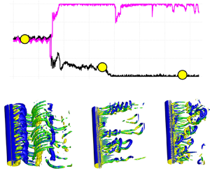
Figure 3. Task I: comparison between DRL from scratch and TL at different  $Re$. (a) Learning from scratch at $Re_D=10^4$; (b) TL $Re_D=10^4$; (c) TL at $Re_D=1.4 \times 10^5$; (d) vortex shedding pattern, the control cylinders are stationary (a,b), and the pattern at the 125th episode (d). Note that in (a–c) the pink and black lines are the time traces of actions ( $\bar {\epsilon }/\epsilon ^{max}$, where $\epsilon _{max}=3.66$) on control cylinders 1 and 2. Blue line is the time trace of $C_D$. The agent of the TL was initialized from the saved agent in the previous case at $Re_D=500$, as shown in figure 2.
In particular, in the TL at  $Re_D=10^4$, as shown in figure 3, the TL agent manages to find the correct rotation direction in less than 10 episodes, and as it reaches the 20th episode, the TL starts exploring a new policy, during which both $\epsilon$ and $C_D$ show notable variations, associated with the so-called ‘catastrophic forgetting’ (Kirkpatrick et al. Reference Kirkpatrick2017). After the 55th episode, the TL can make the correct and stable decision.
In task 1, as  $Re_D$ is increased from $10^4$ to $1.4\times 10^5$, the wake behind the main cylinder becomes very complex, although the boundary layer is laminar at both values of $Re_D$. The learning process at $Re_D=1.4\times 10^5$ is very similar to that of $Re_D=10^4$. In 25 episodes, the TL is able to identify the correct rotation directions. At the 50th episode, the rotation speed on control cylinder 1 begins to show variation and and it starts a new exploration, due to the catastrophic forgetting. Around the 80th episode, the rotation speed on control cylinder 2 also starts to vary, but the rotation speeds on both control cylinders quickly return to optimal value, i.e. $|\epsilon _{\pm 1}|=1$.
We would like to emphasize that the high fidelity LES of flow past a cylinder accompanied by two rotating cylinders at  $Re_D=1.4\times 10^5$ are still a challenge. To the best of the authors’ knowledge, the details of the flow pattern have not been studied before. In figure 3(d), the top snapshot exhibits the vortical flow, while the control cylinders remain stationary. The bottom snapshot shows the flow structures at the 125th episode, when the control cylinders are rotating at optimal speed. We see that, as the control cylinder is rotating, the large-scale streamwise braid vortices are mostly replaced by the hairpin vortices emanating from the gap between the main cylinder and control cylinders, and the wake becomes narrower, which is a sign of a smaller $C_D$.
Next we turn our attention to task 2, where the objective is to maximize the system power gain efficiency,  $\eta$, under the condition that $\epsilon _2=-\epsilon _1$. Note that the objective of the current task 2 is similar to the task 2 in our previous study (Fan et al. Reference Fan, Yang, Wang, Triantafyllou and Karniadaki2020), except that, here, we have used the instantaneous $C_f$ obtained from the simulation, while $C_f$ is a pre-defined constant in Fan et al. (Reference Fan, Yang, Wang, Triantafyllou and Karniadaki2020). Nonetheless, our previous study has revealed that it is much more difficult for DRL to identify the optimal control strategy in task 2 than that in task 1. In task 2, we have started from the DRL from scratch using two-dimensional (2-D) simulation at $Re_D=500$. In particular, since the 2-D simulation is relatively inexpensive and fast, we have run 16 simulations concurrently to provide the training data to a single DRL. For the TL at $Re_D=10^4$ and $Re_D=1.4 \times 10^5$, the simulation is very expensive, thus only a single simulation was performed. It is worth noting that $\eta$ at low $Re_D$ is very different from that at high $Re_D$, as shown in Appendix A, thus it is expected that TL in task 2 and task 3 will be more challenging.
Figure 4(a) shows the learning process of DRL from scratch for task 2 at  $Re_D=500$. In particular, the learning process using a single 2-D simulation (a–c) and 16 2-D simulations (d–f) are plotted together. In figure 4(a), DRL manages to find the correct rotation direction after 75 episodes, but it barely makes the optimal decision, although it has been trained over 300 episodes. On the other hand, in the case of 16 simulations running concurrently, as shown in figure 4(d), DRL can identify the correct rotation direction in less than 10 episodes, and is able to make the optimal decision before the 75th episode.

Figure 4. Task 2: TL from 2-D low  $Re_D$ to 3-D high $Re_D$. (a,d) Learning from scratch, $Re_D=500$: left – single client; right – multi-client. Panels (b,e) show TL, $Re_D=10^4$: (a) and (d) are initialized by the corresponding DRL agents shown in panels (a,d), respectively. Panels (c,f) show TL, $Re_D=1.4\times 10^5$, initialized from the agent corresponding to (e). Panel (f) shows visualization of the policy at the 5th, 15th, 25th and 65th episodes. Note in all the simulations here $\epsilon _{max}=3.66$.
Subsequently, the DRL networks trained in figure 4(a,d) are both applied to the TL at  $Re_D=10^4$, and the results are shown in figure 4(b,e). We observe from figure 4(b) that, although the DRL of figure (a) has identified the correct policy, it gives a very chaotic $\epsilon _1$ in the first 60 episodes in TL. On the other hand, as shown in figure 4(e), the TL is able to give the correct rotation direction in less than 10 episodes, and after 30 episodes it has managed to reach the optimal decision. When applied to the simulation flow at $Re=1.4 \times 10^5$, the TL manages to give stable action values after the 30th episode, but in a short period just after the 40th episode and until the end of the simulation, an unstable action is given, as shown by the variation of $\epsilon _1$ and $\eta$ in figure 4(c). To explain the variation of the decision given by the agent, the policy at 5th, 15th, 25th and 65th episodes are visualized in figure 4(f). Specifically, the black boxes $[-0.25, 0.25] \times [0.3,0.8]$, which correspond to the concentrated intervals of $C_L$ and $C_D$, respectively, are highlighted. We observe that the policy in the highlighted regions has not reached the best strategy yet, although the TL has been trained for 70 episodes. Next, we consider the hardest problem of this paper, task 3, with the same objective as that of task 1, but $\epsilon _1$ and $\epsilon _2$ are independent. Again, we start this task from scratch in a 2-D simulation at $Re_D=500$, as shown in figure 5(a,b). Note that, here, 16 2-D simulations were used to provide training data. As shown in figure 5(a,b), the RL agent was able to give correct rotation directions for both controlling cylinders after 50 episodes. Between the 50th and 110th episodes, $\epsilon _2$ gradually approaches $-1$, while $\epsilon _1$ oscillates around 0.7, the combination of which gives rise to $\eta \approx 1.5$. After the 110th episode, the DRL suddenly changes its actions, in a short period of exploration: $\epsilon _1$ changes to 1, $\epsilon _2$ is $-0.5$ and the value of $\eta$ goes down to 1.37. Meanwhile, the DRL does not stop exploration on $\epsilon _1$, as shown by the variation in the black line, starting around the 200th episode. Around the 280th episode, the DRL is able to reach a near optimal decision, as demonstrated by the fact that $\eta$ is close to 1.325, which is the optimal value obtained from task 2.

Figure 5. Task 3:  $\epsilon _1$ and $\epsilon _2$ are independent. (a,c) The DRL from scratch using 16 2-D simulations at $Re_D=500$; (b,d) TL at $Re_D=10^4$. Panels (c,d) where the top row refers to $\epsilon _1$ and the bottom row refers to $\epsilon _2$, shows the policy at the episodes indicated by the black circles in the corresponding figure of upper panel, respectively.
The TL results of task 3 at  $Re_D=10^4$ are plotted in figure 5(b,d). We observe that TL is able to reach the correct decision on rotation directions in less than 10 episodes. As more training data are obtained, $\epsilon _2$ keeps the maximum value 1, and $\epsilon _1$ is gradually increased to around $\epsilon _1=-0.8$, which gives rise to $\eta \approx 0.84$, which is slightly greater than the optimal value $\eta =0.78$, obtained in task 2. The policy contours at the 5th, 50th, 110th, 220th and 285th episodes for $Re_D=500$ and the 5th, 30th, 80th, 100th and 140th episodes for $Re_D=10^4$ are plotted in figures 5(c) and 5(d), respectively. During the learning process, at $Re_D=500$, $C_D$ and $C_L$ are mostly in the range $[0.1,0.6]$ and $[-1.25,-0.75]$, and at $Re_D=10^4$, these two coefficients are mostly in the range $[0.3,0.8]$ and $[-0.5,0.0]$, respectively. The corresponding $C_D$, $C_L$ ranges are highlighted by black boxes in the two figures. We observe that, at both $Re_D$, the policies for $\epsilon _1$ and $\epsilon _2$ both gradually approach the value that results in optimal $\eta$, which clearly shows the exploration and exploitation stages at work.
4. Summary
We have implemented a DRL in the numerical simulation of bluff body flow active control at high Reynolds number ( $Re_D=1.4\times 10^5$). We demonstrated that, by training the DRL using the simulation data at low $Re_D$, and then applying TL at high $Re_D$, the overall learning process can be accelerated substantially. In addition, the study shows that the TL can result in a more stable decision, which is potentially beneficial to the flow control. Moreover, we proposed a multi-client-single-server DRL paradigm that is able to generate training data much faster to quickly discover an optimal policy. While here we focus on a specific external flow, we believe that similar conclusions are valid for wall-bounded flows and different control strategies.
Funding
The work of Z.W. was supported by the Fundamental Research Funds for the Central Universities (DUT21RC(3)063). The work of G.E.K. was supported by the MURI-AFOSR FA9550-20-1-0358 and by the ONR Vannevar Bush Faculty Fellowship (N00014-22-1-2795). The work of X.J. was supported by the Scientific Innovation Program from China Department of education under Grant (DUT22LAB502); the Dalian Department of Science and Technology (2022RG10); the Provincial Key Lab of Digital Twin for Industrial Equipment (85129003) and the autonomous research project of State Key Laboratory of Structural Analysis, optimization and CAE Software for Industrial Equipment (202000).
Declaration of interests
The authors report no conflict of interest.
Author contributions
M.T., G.E.K. and D.F. conceived of the presented idea. M.T. and G.E.K. supervised the findings of this work. Z.W. wrote the code and performed the numerical simulations. X.J. encouraged Z.W. to investigate and provided the funding. All authors contributed to the final version of the manuscript.
Appendix A. Simulation results of control cylinders rotating at constant speed
In this section, the simulation results for the cases where both control cylinders are rotating at constant speed  $|\varOmega |=\epsilon _{{max}}=3.66$. Figure 6(a–d) shows $C_D$ and $C_L$ on the three cylinders at $Re_D=10^4$ and $Re_D=1.4\times 10^5$, respectively. We observe that, with rotating control cylinders, the $C_D$ on the main cylinder at both $Re_D$ is reduced significantly. With $\epsilon _{{max}}=3.66$, the control cylinders are not able to cancel the vortex shedding on the main cylinder, thus $C_L$ on the main cylinder at both $Re_D$ exhibits the frequency of vortex shedding. In particular, at $Re_D=1.4\times 10^5$, the magnitudes of $C_L$ on control cylinders 1 and 2 show notable discrepancy from each other, which leads to symmetry breaking on the average at this $Re_D$. In addition, figure 7 plots $C_f$ on the control cylinders at both $Re_D$. As shown in the figure, at both $Re_D$, on average, the magnitudes of $C_f$ on the control cylinders are different.

Figure 6. Time series of  $C_D$ and $C_L$ on the main and control cylinders: (a,c) $Re_D=10^4$; (b,d) $Re_D=1.4\times 10^5$. Note that the control cylinders are rotating at constant speed at $\epsilon _1=-1$, $\epsilon _2=1$, $\epsilon _{{max}=3.66}$. The red lines are the hydrodynamic force coefficients on the main cylinder, while the blue and pink ones are on control cylinders 1 and 2, respectively.

Figure 7. Time series of frictional coefficient ( $C_f$) on the control cylinders at $Re_D=10^4$ and $Re_D=1.4\times 10^5$, $\epsilon _1=1$, $\epsilon _2=1$, $\epsilon _{{max}=3.66}$.
In order to validate the optimal control strategy given by DRL in task 2 and task 3, additional simulations with  $\epsilon _2=0$, $\epsilon _2=0.6$, $\epsilon _2=0.75$, $\epsilon _2=0.9$ and $\epsilon _2=1.0$ for $Re_D=500$, and $\epsilon _2=0$, $\epsilon _2=0.85$, $\epsilon _2=0.9$ and $\epsilon _2=1.0$ for $Re_D=10^4$ are performed. Figure 8 plots the power gain coefficient $\eta$ as a function of $\epsilon _2$. Note that the value of $\eta$ at $Re=10^4$ has been enlarged by three times in order to show the variation more clearly. We observe that the minimum of $\eta$ for $Re_D=500$ is around $\epsilon _2=0.75$, and it is $\epsilon _2=0.9$ for $Re_D=10^4$.

Figure 8. Power gain coefficient ( $\eta$) varies with $\epsilon$: blue, $Re_D=500$; red, $Re_D=10^4$. Note that, at $Re_D=10^4$, the value of $\eta$ has been enlarged by three times. Here, $\epsilon _{{max}}=3.66$.
Appendix B. Validation of simulation of cylinder flow at high $Re_D$

In order to validate the numerical method (spectral element plus entropy–viscosity), LES of flow past a cylinder at  $Re_D=1.4\times 10^5$ have been performed. The computational domain has a size of $[-12\,D, 16\,D] \times [-10\,D, 10\,D]$ in the streamwise ( $x$) and cross-flow ( $y$) directions, respectively. The domain is partitioned into 2044 quadrilateral elements. The size of elements around the cylinder in the radial direction is $0.0016\,D$ in order to resolve the boundary layer. The domain size in the spanwise ( $z$) direction is $3D$. Uniform inflow velocity is prescribed at the inflow boundary, a homogeneous Neumann boundary condition for velocity and zero pressure is imposed at the outflow boundary, and wall boundary condition is imposed at the cylinder surface and a periodic boundary condition is assumed at all other boundaries. In particular, two simulations of different resolution are performed: LES $^1$, third-order spectral element, 120 Fourier planes, $\Delta t = 1.5 \times 10^{-4}$; LES $^2$, fourth-order spectral element and 160 Fourier planes, $\Delta t = 1.0 \times 10^{-4}$.
Table 1 presents the statistical values of  $\overline {C_D}$, $\overline {C_L}$, $St$,
$St$,  $L_r$ and $\phi _s$ from the simulation at $Re_D=1.4\times 10^5$. We observe that the simulation results agree with the values obtained from literature very well, and the results are not sensitive to the mesh resolution. A further validation with the experimental measurement is shown in figure 9, which plots the mean local $\overline {C_p}$ and $\overline {C_f}$. Again, the simulation results agree with experimental measurement very well. Figure 10 exhibits the comparison between present LES and the experimental measurement by Cantwell & Coles (Reference Cantwell and Coles1983). It could be observed that the LES results of the mean streamwise velocity ${\bar {u}}/{U_{\infty }}$ along horizontal line $y=0$ and vertical line $x/D=1$ are in good agreement with the experiments. Figure 11 shows the streamlines and contours of the mean velocity and Reynolds stress in the near wake. The results shown in the figures agree with figures 5 and 6 of Braza, Perrin & Hoarau (Reference Braza, Perrin and Hoarau2006) well.
Table 1. Sensitivity study of the simulation result to the mesh resolution: flow past a single circular cylinder at  $Re_D=1.4\times 10^5$. Here, $\overline {C_D}$ is the mean drag coefficient, $\overline {C_L}$ is the root-mean-square value of the lift coefficient, $St$ is the Strouhal number, $L_r$ is the length of the recirculation bubble and $\phi _s$ is the separation angle. The (Breuer Reference Breuer2000) LES is case D2. LES $^1$ and LES $^2$ correspond to the mesh resolutions 1 and 2, respectively.


Figure 9. Local pressure and skin friction coefficient at  $Re_D=1.4 \times 10^5$; comparison with the literature. Note that ‘Present LES’ is from the simulation using mesh LES $^2$, ‘Cantwell & Coles experiment’ refers to the experiment by Cantwell & Coles (Reference Cantwell and Coles1983), ‘Achenbach experiment’ refers to the experiment by Achenbach (Reference Achenbach1968).

Figure 10. Validation of the LES: (a) mean centreline velocity  ${\bar {u}}/{U_{\infty }}$; (b) mean velocity ${\bar {u}}/{U_{\infty }}$ at ${x}/{D}=1$; (c) mean turbulent shear stress ${\overline {u^{\prime } v^{\prime }}}/{U_{\infty }^2}$ at ${x}/{D}=1$. Note that ‘Present LES’ is from the simulation using mesh LES $^2$, ‘Cantwell & Coles experiment’ refers to the experiment by Cantwell & Coles (Reference Cantwell and Coles1983).

Figure 11. Validation of the LES: mean velocity and Reynolds stress field. Note that the reference results are shown in the figures agree with figures 5 and 6 of Braza et al. (Reference Braza, Perrin and Hoarau2006). The present simulation results are from the simulation using mesh resolution LES $^2$. (a) Streamlines; (b) $\bar {u}$; (c) $\bar {v}$; (d) $\overline {uu}$; (e) $\overline {vv}$; (f) $\overline {uv}$.


