


1 Introduction
Turbulent boundary layers (TBLs) under the influence of adverse pressure gradients (APGs) are present in many wall-bounded flows of industrial applications such as wings or divergent nozzles, thus their paramount importance within the field of fluid dynamics. This relevance is supported by various and diverse studies which have analysed the effect of APGs on TBLs either experimentally or through the use of simulations. It was Clauser (Reference Clauser1954, Reference Clauser1956) who laid the groundwork of APG TBLs with an experimental study of this type of flow and the definition of the Clauser pressure-gradient parameter to measure the pressure-gradient magnitude in turbulent boundary layers. Additionally, Coles (Reference Coles1956) proposed the law of the wake after assessing several mean-velocity profiles of pressure-gradient (PG) TBLs. Other relevant studies are the ones by Jones & Launder (Reference Jones and Launder1972) and Spalart & Watmuff (Reference Spalart and Watmuff1993), the latter focused on the analysis of various PGs both experimentally and through a direct numerical simulation (DNS). One of the main conclusions by Spalart & Watmuff (Reference Spalart and Watmuff1993) was the vertical shift downwards of the inner-scaled mean-velocity profile in the buffer and beginning of the overlap layers with adverse pressure gradient. At the same time, Nagano, Tagawa & Tsuji (Reference Nagano, Tagawa and Tsuji1993) showed experimentally the significant effect of the APG on the mean flow and the turbulence statistics, and demonstrated the inadequacy of the law of the wall for turbulent boundary layers subjected to pressure gradients. Subsequently, in the experiments of Skåre & Krogstad (Reference Skåre and Krogstad1994) it was found that the production of turbulent kinetic energy in TBLs exposed to a strong APG shows a second peak located in the outer region. This leads to substantial turbulent diffusion towards the wall unlike the zero-pressure-gradient (ZPG) TBL. More recently, the work of Monty, Harun & Marusic (Reference Monty, Harun and Marusic2011) showed that the APG energises the large scales located in the outer region of the TBL, and revealed that the skewness is increased for APG TBLs, a fact that is linked with an increased interaction of the large scales with the small scales in the near-wall region (Marusic, Mathis & Hutchins Reference Marusic, Mathis and Hutchins2010). Moreover, Harun et al. (Reference Harun, Monty, Mathis and Marusic2013) analysed in detail the outer scales of the turbulent boundary layer, suggesting that the energisation of the outer layer due to the pressure gradient is similar to the energisation due to the increment in Reynolds number, an argument that will be discussed in depth in this work. In addition to these experimental studies, there are recent simulations that analyse the effects of adverse pressure gradients in flat plates, such as the studies by Bobke et al. (Reference Bobke, Vinuesa, Örlü and Schlatter2017) and Lee (Reference Lee2017) with constant and moderate APGs, and the research by Kitsios et al. (Reference Kitsios, Sekimoto, Atkinson, Sillero, Borrell, Gungor, Jiménez and Soria2017) and Maciel, Gungor & Simens (Reference Maciel, Gungor and Simens2017) with very strong APGs.
Despite the fact that one of the main applications of APG TBLs is related to the flow over wings at high Reynolds numbers, it was just a few years ago that the available computational power allowed the performing of simulations of the flow over this specific geometry and the reproduction of cases closer to those analysed in previous experiments. In terms of experimental work in this field, one of the first experiments aimed at thoroughly characterising the flow around a wing section was by Pinkerton (Reference Pinkerton1938), who found that the pressure distribution around a NACA4412 airfoil is approximately independent of the Reynolds number. A very well-known experiment focused on analysing the flow over a wing section was the one performed by Coles & Wadcock (Reference Coles and Wadcock1979), in which detailed boundary-layer measurements were performed, and their experiment was later extended by Wadcock (Reference Wadcock1987). The availability of experimental data for the NACA4412 wing section has motivated a number of simulations of this airfoil. One example is the large-eddy simulation (LES) of a NACA4412 performed by Jansen (Reference Jansen1996) at  $Re_{c}=1.64\times 10^{6}$ (i.e. the Reynolds number based on the free-stream velocity, $U_{\infty }$, and the chord length, $c$) which corresponds to one of the first turbulent-structure-resolving simulations of the flow over a wing. Nevertheless, despite this simulation being at a considerably high Reynolds number, other simulations of the flow around a wing section have been performed at lower Reynolds numbers with higher resolution with the aim of resolving the full range of turbulent structures in the flow in order to analyse in detail the characteristics of the turbulent boundary layer. Among these simulations it is worth mentioning the DNS of a NACA0012 at $Re_{c}=50\,000$ by Rodríguez et al. (Reference Rodríguez, Lehmkuhl, Borrell and Oliva2013), the DNS by Hosseini et al. (Reference Hosseini, Vinuesa, Schlatter, Hanifi and Henningson2016) of a NACA4412 at $Re_{c}=400\,000$ and $5^{\circ }$ angle of attack or the LES by Sato et al. (Reference Sato, Asada, Nonomura, Kawai and Fujii2016) of a NACA0015 at $Re_{c}=1\,600\,000$, among others. Additionally, Vinuesa et al. (Reference Vinuesa, Negi, Atzori, Hanifi, Henningson and Schlatter2018) carried out the comparison of the APG TBLs in a NACA4412 at different Reynolds numbers (ranging from 100 000 to 1 000 000), obtaining results that suggest that the effect of the APG is attenuated as the Reynolds number of the flow is increased.
The main goal of the present study is to analyse the effect of the adverse pressure gradient and the flow history on the turbulent boundary layers developing on the suction side of two airfoils: the cambered NACA4412 and the symmetric NACA0012 both at  $Re_{c}=400\,000$, with $5^{\circ }$ and $0^{\circ }$ angle of attack, respectively. This can be considered as the continuation of the work by Vinuesa et al. (Reference Vinuesa, Hosseini, Hanifi, Henningson and Schlatter2017a) but now comparing two cases with different pressure distributions over the surface of the wing. The relevance of this work lies in the assessment of the effects that different APG magnitudes (mild in the NACA0012 and strong in the NACA4412) and flow histories have on the turbulent boundary layer, both in terms of turbulence statistics and of the most energetic scales.
The present paper is organised as follows: the details of the numerical method and the databases used for the assessment of the results are presented in § 2; the integral properties and the turbulence statistics of the cases under study are discussed in § 3; one- and two-dimensional spectral analyses are shown in § 4; and the summary of the paper together with the main conclusions of the study are included in § 5.
2 Computational set-up and databases
The present simulations of TBLs on two wing sections have been performed with the open-source incompressible Navier–Stokes solver Nek5000, developed by Fischer, Lottes & Kerkemeier (Reference Fischer, Lottes and Kerkemeier2008). This code is based on the spectral-element method first introduced by Patera (Reference Patera1984), which combines the advantages of the finite-element method and spectral methods, i.e. geometry flexibility and high accuracy, respectively. The spatial discretisation is based on Lagrange interpolants of polynomial order  $N=11$, where the points within the element are distributed in terms of the Gauss–Lobatto–Legendre (GLL) quadrature points, and it follows the $\mathbb{P}_{N}-\mathbb{P}_{N-2}$ formulation (i.e. the interpolants for the pressure are of polynomial order $N-2$). Concerning time-stepping implementation, the viscous terms are solved implicitly by means of the third-order backward differentiation scheme (BDF3), whereas the nonlinear terms are solved explicitly by third-order extrapolation (EXT3). In addition, in order to avoid aliasing errors, overintegration is performed by oversampling the nonlinear terms by a factor of $3/2$ in each direction.
The TBLs of both cases are simulated through the use of well-resolved LESs which accurately solve for the largest scales of the turbulent flow whereas the smallest scales are modelled with a subgrid-scale (SGS) model developed by Schlatter, Stolz & Kleiser (Reference Schlatter, Stolz and Kleiser2004). The approach in this method is based on a relaxation-term filter which adds a dissipative force accounting for the dissipation of the unresolved turbulent scales in the simulation. The numerical set-up employed in this work, with the mesh resolution discussed below and the relaxation-term SGS model, was thoroughly validated by Negi et al. (Reference Negi, Vinuesa, Hanifi, Schlatter and Henningson2018) against the fully resolved DNS data of the NACA4412 wing section at  $Re_{c}=400\,000$ by Hosseini et al. (Reference Hosseini, Vinuesa, Schlatter, Hanifi and Henningson2016). In this study approximately 90 % of the total dissipation of turbulent kinetic energy (TKE) is resolved by the LES while the remaining 10 % is added by the SGS model.

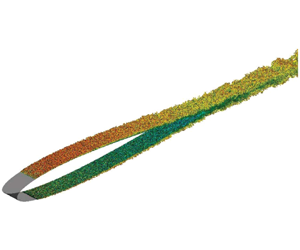
Figure 1. (a) Two-dimensional spectral-element mesh, without the GLL points, used in the simulation of the NACA0012 wing section. (b) Instantaneous visualisation of the NACA0012 case showing coherent vortical structures identified through the  $\unicode[STIX]{x1D706}_{2}$ method (Jeong & Hussain Reference Jeong and Hussain1995). The vortical structures are coloured by their streamwise velocity from low (blue) to high (red) velocity.
As stated previously, the cases under study are the flows around NACA4412 and NACA0012 airfoils. In order to achieve the desired well-resolved LES resolution, the spatial resolution near the wall is expressed in terms of viscous units such that  $\unicode[STIX]{x0394}x_{t}^{+}=18.0$, $\unicode[STIX]{x0394}y_{n}^{+}=(0.64,11.0)$ and $\unicode[STIX]{x0394}z^{+}=9.0$ (here $t$ and $n$ denote the directions tangential and normal to the wing surface); whereas the spatial resolution in the wake follows $\unicode[STIX]{x0394}x/\unicode[STIX]{x1D702}<9$, where $\unicode[STIX]{x1D702}=(\unicode[STIX]{x1D708}^{3}/\unicode[STIX]{x1D700})^{1/4}$ stands for the Kolmogorov scale (note that $\unicode[STIX]{x1D708}$ is the fluid kinematic viscosity and $\unicode[STIX]{x1D700}$ the local isotropic dissipation). The mesh design strategy is similar to that by Hosseini et al. (Reference Hosseini, Vinuesa, Schlatter, Hanifi and Henningson2016), with a slightly coarser resolution because in this case we perform a well-resolved LES, as discussed by Vinuesa et al. (Reference Vinuesa, Negi, Atzori, Hanifi, Henningson and Schlatter2018). The scaling in viscous units is defined in terms of the friction velocity $u_{\unicode[STIX]{x1D70F}}=\sqrt{\unicode[STIX]{x1D70F}_{w}/\unicode[STIX]{x1D70C}}$ (where $\unicode[STIX]{x1D70F}_{w}$ is the mean wall-shear stress and $\unicode[STIX]{x1D70C}$ the fluid density) and the viscous length $l^{\ast }=\unicode[STIX]{x1D708}/u_{\unicode[STIX]{x1D70F}}$. The domain under consideration is a C-mesh (as shown in figure 1a) with streamwise length $L_{x}=6c$, vertical length $L_{y}=4c$ and spanwise length $L_{z}=0.1c$. Vinuesa et al. (Reference Vinuesa, Hosseini, Hanifi, Henningson and Schlatter2017a) concluded that this computational domain is wide enough to contain the relevant scales in the TBL on the suction side of the NACA4412 by analysing the spanwise power-spectral density distributions. Furthermore, figure 1(b) shows an instantaneous field of the coherent vortices identified by the $\unicode[STIX]{x1D706}_{2}$ criterion (Jeong & Hussain Reference Jeong and Hussain1995) and it can be observed that the boundary layer is tripped at 10 % chord-length distance from the leading edge on both the suction and pressure sides of the wing section. The tripping consists of a wall-normal random-volume forcing which spans the whole domain in $z$, following the approach by Schlatter & Örlü (Reference Schlatter and Örlü2012). Concerning the boundary conditions, the procedure used by Hosseini et al. (Reference Hosseini, Vinuesa, Schlatter, Hanifi and Henningson2016) is adopted such that all the boundaries, except the outlet, are set as Dirichlet boundary conditions extracted from a previous Reynolds-averaged Navier–Stokes (RANS) simulation. This RANS simulation is performed using the $k{-}\unicode[STIX]{x1D714}$ shear-stress transport model by Menter (Reference Menter1994) performed with the software ANSYS Fluent in a circular domain with 200 chord-length radii. This RANS model has been shown to adequately predict pressure-gradient (PG) effects on TBLs. Although the effect of using such a Dirichlet boundary condition on the turbulence statistics and the power-spectral densities is minor, future extensions of this work will make use of adaptive mesh refinement strategies aimed at significantly extending the computational domain (Tanarro et al. Reference Tanarro, Mallor, Offermans, Peplinski, Vinuesa and Schlatter2019). On the other hand, the boundary condition at the outflow corresponds to the one developed by Dong, Karniadakis & Chryssostomidis (Reference Dong, Karniadakis and Chryssostomidis2014) which removes any energy inflow into the domain. The initial condition of the simulation is the RANS simulation solution, nevertheless, in order to remove the transients from the simulation before starting to collect statistical values and time series, the simulation is run for 4 flow-over times using interpolants of polynomial order $N=5$ and, subsequently, 2 flow-over times with a polynomial order $N=7$. After this, the simulations are run with the full resolution (i.e. $N=11$) and turbulence statistics are collected by spanwise and temporal averaging. The temporal averaging in both cases is performed over 9 flow-over times (note that we exploit the flow symmetry in the NACA0012 case, and therefore the effective average time is longer in this case). The temporal averaging can be further expressed in terms of the normalised eddy-turnover time $\text{ETT}^{\ast }=tu_{\unicode[STIX]{x1D70F}}/\unicode[STIX]{x1D6FF}_{99}L_{z}/L_{z,ref}$ as discussed by Vinuesa et al. (Reference Vinuesa, Negi, Atzori, Hanifi, Henningson and Schlatter2018). Here $t$ is the flow-over time (scales with $U_{\infty }$ and $c$) and $\unicode[STIX]{x1D6FF}_{99}$ is the boundary-layer thickness. This definition of the eddy-turnover time takes into account the length of the domain in the homogeneous direction (i.e. in this case $L_{z}$) with respect to a reference length $L_{z,ref}=3\unicode[STIX]{x1D6FF}_{99}$ described by Flores & Jiménez (Reference Flores and Jiménez2010) as the minimum box size required to contain the largest structures in the logarithmic region. According to the high- $Re$ DNS of ZPG TBLs performed by Sillero, Jiménez & Moser (Reference Sillero, Jiménez and Moser2014), convergence of the turbulence statistics can be considered for, approximately, 12 eddy-turnover times, whereas the averaging periods in the simulations of the NACA4412 and the NACA0012 are $\text{ETT}^{\ast }=18$ and 65 at $x_{ss}/c=0.8$, respectively. This ensures the convergence of the statistics shown here. Regarding the size of the cases, the mesh of the NACA4412 has 270 000 spectral elements whereas the NACA0012 mesh is formed by 220 000 spectral elements, giving as result a total of 466 million and 380 million grid points, respectively.
Aside from the two wing sections simulated in this work, the results will be compared with additional databases, namely the LES of a ZPG TBL by Eitel-Amor, Örlü & Schlatter (Reference Eitel-Amor, Örlü and Schlatter2014) and the flat-plate TBLs subjected to APGs obtained by Bobke et al. (Reference Bobke, Vinuesa, Örlü and Schlatter2017), in order to have a more complete assessment of the effect of flow history on TBLs.
3 Integral quantities and turbulence statistics
As discussed in the introduction, the main goal of this paper is to assess the effect of APG and flow history on TBLs, therefore, several quantities will be analysed in terms of these effects. First, the integral properties of the boundary layer such as pressure-gradient magnitude, friction Reynolds number ( $Re_{\unicode[STIX]{x1D70F}}$), momentum-thickness Reynolds number ( $Re_{\unicode[STIX]{x1D703}}$) and others will be presented and assessed both on the suction side of the wing (denoted by the subscript ss) and the pressure side (denoted by the subscript ps). Note that $Re_{\unicode[STIX]{x1D70F}}=\unicode[STIX]{x1D6FF}_{99}u_{\unicode[STIX]{x1D70F}}/\unicode[STIX]{x1D708}$ and $Re_{\unicode[STIX]{x1D703}}=U_{e}\unicode[STIX]{x1D703}/\unicode[STIX]{x1D708}$, where $\unicode[STIX]{x1D6FF}_{99}$ and $U_{e}$ are the 99 % boundary-layer thickness and the mean velocity at the boundary-layer edge (both obtained using the method outlined by Vinuesa et al. (Reference Vinuesa, Bobke, Örlü and Schlatter2016)), and $\unicode[STIX]{x1D703}$ is the momentum thickness. Second, the turbulence statistics gathered from the simulation are shown. These turbulence statistics include the mean-velocity profiles, the non-zero components of the Reynolds-stress tensor and the TKE budgets. Note that the specific effects of curvature are not analysed since these are dominated by the pressure-gradient effects (Patel & Sotiropoulos Reference Patel and Sotiropoulos1997).
3.1 Integral quantities
In order to assess the effect of the APG on TBLs we first need to define a parameter to measure its magnitude. This measurement is made in terms of the Clauser pressure-gradient parameter  $\unicode[STIX]{x1D6FD}=\unicode[STIX]{x1D6FF}^{\ast }/\unicode[STIX]{x1D70F}_{w}\,\text{d}P_{e}/\text{d}x_{t}$, where $\unicode[STIX]{x1D6FF}^{\ast }$ is the displacement thickness and $P_{e}$ is the pressure at the boundary-layer edge (Clauser Reference Clauser1954, Reference Clauser1956). Figure 2(a) shows the evolution of the Clauser pressure-gradient parameter along the chord on both sides of the wing sections (recall that the NACA0012 at $0^{\circ }$ angle of attack is a symmetric case and the results shown here are based on that symmetry). First, note that the computation of $\unicode[STIX]{x1D6FD}$ is started at, approximately, $x/c=0.2$. The reason is that, as mentioned above, the calculation of $\unicode[STIX]{x1D6FF}_{99}$ is based on the diagnostic scaling (Vinuesa et al. Reference Vinuesa, Bobke, Örlü and Schlatter2016), which requires the turbulent intensity. Thus, it can only be used after the boundary layer becomes fully turbulent, i.e. after approximately $x/c=0.2$ from the leading edge. Therefore, all those quantities that depend on the boundary-layer thickness or boundary-layer edge velocity will be computed at those locations. With respect to the results shown in figure 2(a), it can be observed that the pressure side of the NACA4412 shows, for most of the surface, a negative value of $\unicode[STIX]{x1D6FD}$ which corresponds to a favourable pressure gradient (FPG). Second, regarding the NACA0012 and the suction side of the NACA4412, it is clear that the NACA4412 exhibits a much stronger APG with respect to the NACA0012, due to the airfoil camber and the angle of attack.

Figure 2. Clauser pressure-gradient parameter  $\unicode[STIX]{x1D6FD}$ as a function of (a) the distance from the leading edge and (b) the friction Reynolds number. The black circle on (b) indicates the case in which the NACA0012 and the NACA4412 exhibit matching local values of $\unicode[STIX]{x1D6FD}$ and $Re_{\unicode[STIX]{x1D70F}}$.
Apart from the assessment of APG effects on TBLs, the other aim of this paper is to analyse the effect of the flow history, i.e.  $\unicode[STIX]{x1D6FD}(x)$. In order to account for this effect, we define an integrated APG magnitude, $\overline{\unicode[STIX]{x1D6FD}}(Re_{\unicode[STIX]{x1D703}})=(Re_{\unicode[STIX]{x1D703}}-Re_{\unicode[STIX]{x1D703},0})^{-1}\int _{Re_{\unicode[STIX]{x1D703},0}}^{Re_{\unicode[STIX]{x1D703}}}\unicode[STIX]{x1D6FD}(Re_{\unicode[STIX]{x1D703}})\,\text{d}Re_{\unicode[STIX]{x1D703}}$ (where $Re_{\unicode[STIX]{x1D703},0}$ defines the point where the integration is started), as a function of the momentum-thickness Reynolds number. This method was first proposed by Vinuesa et al. (Reference Vinuesa, Örlü, Sanmiguel Vila, Ianiro, Discetti and Schlatter2017b), who were able to obtain the skin-friction curve of APG TBLs by using this parameter and ZPG TBL data. In the evaluation of flow-history effects it is desired that local APG and Reynolds-number effects are avoided. Figure 2(b) shows that there is only one case in which we have the same local APG magnitude ( $\unicode[STIX]{x1D6FD}\simeq 3.5$) and same friction Reynolds number ( $Re_{\unicode[STIX]{x1D70F}}\simeq 362$) for both wing sections. This will be considered as the matching $\unicode[STIX]{x1D6FD}{-}Re_{\unicode[STIX]{x1D70F}}$ case which will allow the analysis of the flow history effect on the TBL. Note that this specific case requires the results of the NACA0012 at $x_{ss}/c=0.95$ for which $\text{ETT}^{\ast }=30$, therefore convergence of the results at this location is ensured.

Figure 3. Normalised pressure coefficient  $C_{p}$ for the two wing sections under study as a function of the distance from the leading edge.

Figure 4. Streamwise evolution of (a) the friction Reynolds number and (b) the momentum-thickness Reynolds number.
Figure 3 shows the pressure coefficient,  $C_{p}$, along the chord of the NACA4412, both on the pressure and suction sides, and the NACA0012 (note that the $C_{p}$ is the same on both sides). The pressure coefficient is presented in normalised form, where the pressure coefficient at the stagnation point $C_{p,st}$ is unity, therefore $C_{p,st}=(P_{st}-P_{\infty })/(1/2\unicode[STIX]{x1D70C}U_{\infty }^{2})=1$. This is achieved by setting the ambient pressure $P_{\infty }$ to fulfil this equation. The $C_{p}$ distributions show a very clear trend with respect to the level of pressure gradient. Near the leading edge, the lowest $C_{p}$ corresponds to the case with higher curvature (i.e. the NACA4412 wing section on the suction side) in which the flow is most accelerated. Nevertheless, as the flow approaches the trailing edge, the effect of the APG can be clearly distinguished. The suction side of the NACA4412 (i.e. the region with the strongest APG) exhibits a higher rate of increase in $C_{p}$ due to the flow being decelerated by the APG. On the other hand, on the pressure side of the NACA4412, which is subjected to a favourable pressure gradient, the $C_{p}$ trend decreases along the chord as the flow is accelerated due to the FPG. Lastly, the NACA0012, which corresponds to a mild APG, shows a decreasing $C_{p}$ along the chord but at a slower rate than on the suction side of the NACA4412.
Figure 4(a) shows the streamwise evolution of the friction Reynolds number, which is also computed after  $x/c=0.2$ as discussed above. It can be observed that the friction Reynolds number in the FPG TBL shows continuous growth along the surface of the wing section whereas both APG TBLs show an initial increase in friction Reynolds number up to a point where it starts to decrease. In the case of the NACA0012 (i.e. mild APG), there is a subtle decrease of $Re_{\unicode[STIX]{x1D70F}}$ at, approximately, $x_{ss}/c=0.9$ after reaching a maximum value of $Re_{\unicode[STIX]{x1D70F}}=372$ while the TBL of the NACA4412 (i.e. strong APG) shows a steep reduction of $Re_{\unicode[STIX]{x1D70F}}$ which begins at, approximately, $x_{ss}/c=0.8$ where $Re_{\unicode[STIX]{x1D70F}}=369$. This decreasing behaviour is the result of the APG becoming very strong and reducing significantly the skin friction. On the other hand, the momentum-thickness Reynolds number $Re_{\unicode[STIX]{x1D703}}$ is presented in figure 4(b). In this case, all the boundary layers show an increasing $Re_{\unicode[STIX]{x1D703}}$ behaviour, the growth rate being larger for increasing APG. This is directly related to the increase in the mean streamwise velocity deficit of the boundary layer due to the presence of the APG.
Other integral properties of interest in the assessment of the APG effect on TBLs are the skin-friction coefficient  $C_{f}=2(u_{\unicode[STIX]{x1D70F}}/U_{e})^{2}$ and the shape factor $H=\unicode[STIX]{x1D6FF}^{\ast }/\unicode[STIX]{x1D703}$. In figure 5(a) we show the skin-friction coefficient of the wing sections as a function of $Re_{\unicode[STIX]{x1D703}}$, together with the ZPG correlation of this value obtained by Nagib, Chauhan & Monkewitz (Reference Nagib, Chauhan and Monkewitz2007). The figure shows that the APG TBLs exhibit an almost constant decrease of the skin-friction coefficient while the skin-friction reduction in the ZPG is not so strong as $Re_{\unicode[STIX]{x1D703}}$ increases. It can be observed that the trend of $C_{f}$ for both wing sections is similar and it can also be noted that there is no mean separation of the flow along the wing sections since the skin-friction coefficient does not show negative values for any of the cases analysed. Figure 5(b) shows the evolution of the shape factor as a function of $Re_{\unicode[STIX]{x1D703}}$, together with the ZPG correlation by Monkewitz, Chauhan & Nagib (Reference Monkewitz, Chauhan and Nagib2007). Note that the ZPG trend exhibits the expected decreasing behaviour with $Re_{\unicode[STIX]{x1D703}}$, whereas both APG TBLs show an increasing trend related to the thickening of the boundary layer due to the APG.
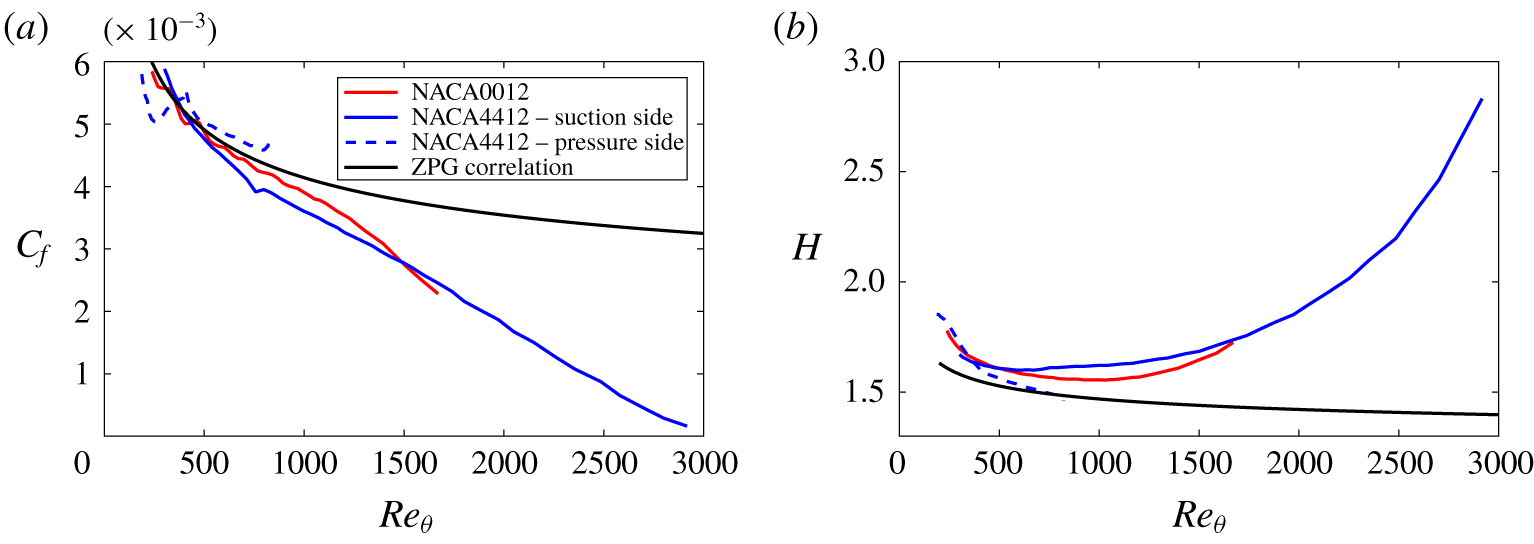
Figure 5. Evolution of (a) the skin-friction coefficient and (b) the shape factor as a function of the momentum-thickness Reynolds number. The results of the ZPG are computed by means of correlations obtained by Nagib et al. (Reference Nagib, Chauhan and Monkewitz2007) for  $C_{f}$ and by Monkewitz et al. (Reference Monkewitz, Chauhan and Nagib2007) for $H$.
$H$.
Table 1 shows the values of the integral parameters discussed above for the two wing cases at several streamwise positions, together with selected ZPG profiles from the database by Eitel-Amor et al. (Reference Eitel-Amor, Örlü and Schlatter2014) at approximately matching  $Re_{\unicode[STIX]{x1D70F}}$, which will be analysed in detail below.
Table 1. List of analysed cases with the corresponding integral properties. ZPG data at similar  $Re_{\unicode[STIX]{x1D70F}}$ from the database by Eitel-Amor et al. (Reference Eitel-Amor, Örlü and Schlatter2014). The case with matched $\unicode[STIX]{x1D6FD}$ and $Re_{\unicode[STIX]{x1D70F}}$ values is indicated in figure 2.

3.2 Turbulence statistics
In this section we focus on the analysis of the most relevant turbulence statistics computed from the simulations. As discussed in § 2, the turbulence statistics were obtained by spanwise and temporal averaging. The terms required to compute all the statistical terms are first expressed in the spectral-element mesh, and then spectrally interpolated on profiles normal to the wing surface. The statistics are expressed in terms of the directions tangential ( $t$) and normal ( $n$) to the wing surface. The comparison with the ZPG TBL follows the proposal by Monty et al. (Reference Monty, Harun and Marusic2011) of analysing cases with matching $Re_{\unicode[STIX]{x1D70F}}$.
3.2.1 Tangential mean-velocity profiles
Figure 6 shows the tangential mean-velocity profiles of the cases described in table 1. We first focus on the cases at matched  $x_{ss}/c=0.4$ and 0.75, in which both the local $\unicode[STIX]{x1D6FD}$ and the integrated APG magnitude differ. The first finding is that the wake region is more prominent for higher APG, as observed among others by Spalart & Watmuff (Reference Spalart and Watmuff1993), Monty et al. (Reference Monty, Harun and Marusic2011): in the cases at $x_{ss}/c=0.4$ the effect is mild, especially in the NACA0012; however, at $x_{ss}/c=0.75$, this effect is significant in both wings, especially in the NACA4412 due to the stronger APG. Another observation that can be drawn from these plots is the effect of the APG on the buffer region of the turbulent boundary layer. Despite the fact that this effect cannot be observed at $x_{ss}/c=0.4$, the stronger APGs at $x_{ss}/c=0.75$ exhibit a significant shift of the inner-scaled mean velocity downwards within the buffer layer at increasing APG, an effect first reported by Spalart & Watmuff (Reference Spalart and Watmuff1993), which may be overemphasised in low-Reynolds-number boundary layers. Besides the shift in the inner-scaled mean velocity by the APG, the profiles also exhibit a larger slope in the overlap region as shown in the insets in figure 6(a,b) with increasing APG, as observed by Spalart & Watmuff (Reference Spalart and Watmuff1993) and Vinuesa et al. (Reference Vinuesa, Hosseini, Hanifi, Henningson and Schlatter2017a) among others, and analysed by Nagib & Chauhan (Reference Nagib and Chauhan2008) through the characterisation of the dependence of the von Kármán coefficient $\unicode[STIX]{x1D705}$ on flow geometry and pressure gradient. These effects are related to effect of the APG on the large-scale structures (Maciel et al. Reference Maciel, Gungor and Simens2017; Sanmiguel Vila et al. Reference Sanmiguel Vila, Örlü, Vinuesa, Schlatter, Ianiro and Discetti2017), which affect the momentum transfer across the whole boundary layer (Vinuesa et al. Reference Vinuesa, Hosseini, Hanifi, Henningson and Schlatter2017a).

Figure 6. Inner-scaled tangential mean-velocity profiles at (a)  $x_{ss}/c=0.4$ and (b) $x_{ss}/c=0.75$. (c,d) Show the case with matched $\unicode[STIX]{x1D6FD}$ and $Re_{\unicode[STIX]{x1D70F}}$ values, in inner and outer scaling respectively. Refer to table 1 for the parameters of the cases.

Figure 7. Inner-scaled non-zero Reynolds stresses corresponding to (a)  $x_{ss}/c=0.4$ and (b) $x_{ss}/c=0.75$. (c,d) Show the case with matched $\unicode[STIX]{x1D6FD}$ and $Re_{\unicode[STIX]{x1D70F}}$ values, in inner and outer scaling respectively. The colours indicate: tangential (—— (blue)), wall-normal (—— (red)), spanwise (—— (green)) velocity fluctuations and Reynolds-shear stress (—— (black)). Refer to table 1 for the parameters of the cases.
On the other hand, figure 6(c,d) shows the mean velocity profile at matching  $\unicode[STIX]{x1D6FD}-Re_{\unicode[STIX]{x1D70F}}$ conditions with different scalings. The inner-scaled mean-velocity profiles show a different trend when compared with the other two cases regarding the behaviour in the buffer layer, i.e. the velocity in the buffer layer is slightly lower in the ZPG than in the NACA0012 at this location. This in principle would also contradict the results by Spalart & Watmuff (Reference Spalart and Watmuff1993), although it can be argued that at this particular location the viscous units may not be adequate to scale the profile in the NACA0012 case due to the fact that, as shown in figure 2(b), here, the friction Reynolds-number curve starts to show a decreasing trend. This suggests that, under these conditions, inner scaling may be inappropriate, as also reported by Maciel et al. (Reference Maciel, Wei, Gungor and Simens2018). Therefore, for the matching $\unicode[STIX]{x1D6FD}{-}Re_{\unicode[STIX]{x1D70F}}$ case we will use the outer scaling based on $U_{e}$. It can then be observed in figure 6(d) that the outer-scaled mean velocity of the ZPG on the buffer and overlap regions is much higher than the APG cases, where the flow is significantly decelerated. Furthermore, when comparing both wing sections (both with same local APG and $Re_{\unicode[STIX]{x1D70F}}$), the mean-velocity profile of the NACA4412 is shifted downwards in the buffer layer, suggesting that the flow history (i.e. the integrated APG) has a noticeable effect in the mean-velocity profiles.
3.2.2 Reynolds stresses
Further understanding of APG and flow-history effects on turbulent boundary layers can be acquired through the analysis of the Reynolds-stress tensor. Figure 7 shows the non-zero Reynolds stresses for each of the cases included in table 1. Following the same procedure as for the mean-velocity profiles, we first focus on the analysis of the profiles at  $x_{ss}/c=0.4$ and $x_{ss}/c=0.75$, shown in (a) and (b) respectively. Already at $x_{ss}/c=0.4$ the effect of the APG is noticeable, and at $x_{ss}/c=0.75$ the effect becomes greatly intensified. The inner-scaled near-wall peak of the tangential velocity fluctuations increases with the APG (as previously documented for instance by Monty et al. (Reference Monty, Harun and Marusic2011)). In addition, the APG has an even more significant effect on the outer region of the boundary layer, exhibiting an outer peak for very strong APG TBLs (Skåre & Krogstad Reference Skåre and Krogstad1994) in the tangential component of the velocity fluctuations, but also larger intensities in the other terms of the Reynolds-stress tensor. This is linked to the energisation of the outer region of the boundary layer in the presence of an APG (Harun et al. Reference Harun, Monty, Mathis and Marusic2013).
In the matching  $\unicode[STIX]{x1D6FD}{-}Re_{\unicode[STIX]{x1D70F}}$ case we encounter a situation similar to that of the mean flow regarding the scaling in inner units. In particular, we observe that the NACA0012, which has been subjected to a milder accumulated APG than the NACA4412, exhibits a stronger inner-scaled near-wall peak. Due to the complexity of flow-history effects, it is not clear whether the accumulated effect of $\unicode[STIX]{x1D6FD}$ affects the inner and outer regions equally, and given the fact that the $Re_{\unicode[STIX]{x1D70F}}$ shows a decreasing trend in the NACA0012 case at this location, inner scaling might not be the most appropriate choice. In order to obtain additional insight into the inner and outer regions in these two boundary layers, we scale the components of the Reynolds-stress tensor in outer units. This approach was also adopted by Harun et al. (Reference Harun, Monty, Mathis and Marusic2013) in their APG experiment, to show that the observed larger values of the streamwise velocity fluctuations were not due to the lower friction velocity, which is a consequence of the APG, but due to more intense large-scale turbulent fluctuations. Harun et al. (Reference Harun, Monty, Mathis and Marusic2013) reached the conclusion that, in outer scaling, the outer peak of the streamwise velocity fluctuations increases with APG magnitude, whereas the near-wall peak exhibits the opposite trend. This is associated with the increased wall-normal convection of near-wall turbulence, which is also produced by the APG, and as will be discussed below affects the power-spectral density in the outer region. Interestingly, when using the edge velocity $U_{e}$ to scale the Reynolds stresses in figure 7(d) we can observe a behaviour similar to the one reported by Harun et al. (Reference Harun, Monty, Mathis and Marusic2013), where the NACA4412 profile, subjected to the strongest accumulated APG, exhibits the largest outer peak and the smallest peak in the near-wall region. Note that in this study we employ the edge velocity $U_{e}$ for outer scaling given the fact that in PG TBLs there is not a clear definition of the outer velocity scale (unlike in ZPGs, where the free-stream velocity is constant), since the streamwise pressure gradient leads to a mean velocity gradient for $y_{n}>\unicode[STIX]{x1D6FF}_{99}$. Furthermore, Vinuesa et al. (Reference Vinuesa, Bobke, Örlü and Schlatter2016) argued that $U_{e}$, obtained using the method reported in their study, constitutes a robust outer scale over a wide range of Reynolds numbers and pressure gradients.
In order to further assess the effect of APG and flow history on TBLs, the database by Bobke et al. (Reference Bobke, Vinuesa, Örlü and Schlatter2017) will be added to the analysis. In particular, we will consider the cases with constant values of  $\unicode[STIX]{x1D6FD}(x)=1$ and 2 over significant parts of the simulation domain. For the purpose of the present work, these flat-plate cases exhibit an approximately 3 % variation in $\unicode[STIX]{x1D6FD}$ in the areas of interest, i.e. from points II to I and from IV to III in the $\unicode[STIX]{x1D6FD}=1$ and 2 cases, respectively. Note that due to the transition from laminar to turbulent flow produced by the tripping, the integrated APG magnitude $\overline{\unicode[STIX]{x1D6FD}}$ is computed by integrating from the location at which the flow can be considered to be turbulent, i.e. at approximately $Re_{\unicode[STIX]{x1D70F}}\simeq 150$. Here, we consider a lower limit in $Re$ than that of Vinuesa et al. (Reference Vinuesa, Örlü, Sanmiguel Vila, Ianiro, Discetti and Schlatter2017b) in order to have a sufficient integration length for some of the matching cases discussed below. Although the resulting values of $\overline{\unicode[STIX]{x1D6FD}}$ vary with the choice of the origin for integration, the trends documented below do not depend on this particular choice. Figure 8 shows the four conditions in which there are matching $\unicode[STIX]{x1D6FD}{-}Re_{\unicode[STIX]{x1D70F}}$ cases between the flat plates and the wing sections. Additional information from these four cases is provided in table 2, with the corresponding $\overline{\unicode[STIX]{x1D6FD}}$ values.
Figure 9 shows the inner-scaled tangential velocity fluctuations for the cases summarised in table 2. This specific Reynolds-stress tensor component has been selected because it allows us to analyse the effect of the flow history both on the near-wall peak and the outer region. The first observation that can be made is the almost negligible effect of the integrated APG magnitude  $\overline{\unicode[STIX]{x1D6FD}}$ on the near-wall peak, where only small differences among cases can be observed. This result suggests that the inner peak scaled in wall units is not closely related to the accumulated flow history, but its deviation with respect to the ZPG curve indicates that it is more strongly dependent on the local APG magnitude $\unicode[STIX]{x1D6FD}$. This would indicate that the near-wall region adapts more quickly to the imposed pressure gradient than the outer region (Bobke et al. Reference Bobke, Vinuesa, Örlü and Schlatter2017). The other observation that can be made from these results is the strong effect of the flow history (i.e. the integrated $\overline{\unicode[STIX]{x1D6FD}}$) on the outer region of the boundary layer, showing consistency with the fact that the inner-scaled tangential velocity fluctuations in the outer layer increase in magnitude with larger integrated APG magnitudes.

Figure 8. Clauser pressure-gradient parameter as a function of the friction Reynolds number on the two wing sections and two of the flat-plate APG cases by Bobke et al. (Reference Bobke, Vinuesa, Örlü and Schlatter2017). The Roman numerals indicate the various matching cases under study.
Table 2. Data from the wing sections and APG flat plates (Bobke et al. Reference Bobke, Vinuesa, Örlü and Schlatter2017) at matching local values of  $\unicode[STIX]{x1D6FD}$ and $Re_{\unicode[STIX]{x1D70F}}$ indicated in figure 8 with Roman numerals from I to IV.


Figure 9. Inner-scaled tangential velocity fluctuations for cases (a) I, (b) II, (c) III and (d) IV (as defined in figure 8). Refer to table 2 for the description of the cases. The constant- $\unicode[STIX]{x1D6FD}$ and ZPG cases are obtained from Bobke et al. (Reference Bobke, Vinuesa, Örlü and Schlatter2017) and from Schlatter et al. (Reference Schlatter, Li, Brethouwer, Johansson and Henningson2010), respectively.

Figure 10. (a,c,e) Turbulent kinetic energy budgets and (b,d,f) production of  $\overline{u_{t}^{2}}$ and $\overline{u_{n}^{2}}$. Profiles at (a,b) $x_{ss}/c=0.4$, (c,d) $x_{ss}/c=0.75$ (in inner scaling) and (e,f) case at matched $\unicode[STIX]{x1D6FD}$ and $Re_{\unicode[STIX]{x1D70F}}$ values (in outer scaling). The colours in the left panels correspond to: production (—— (blue)), dissipation (—— (red)), turbulent transport (—— (green)), viscous diffusion (—— (brown)), velocity–pressure-gradient correlation (—— (black)) and convection (—— (magenta)).
3.2.3 Turbulent kinetic energy budgets
Following the assessment of the mean flow and the Reynolds stresses, we now analyse the effect of the APG and flow history on the TKE budget terms across the TBL. In figure 10(a,c,e) we show the TKE budgets for the cases listed in table 1. Among the main results, the APG has a significant effect on the turbulent production across the boundary layer but most remarkably in the outer region, where strong APGs exhibit an outer peak. This result was already observed in the experiment by Skåre & Krogstad (Reference Skåre and Krogstad1994), who linked the emergence of the outer peak in turbulent production with the increase in turbulent shear stresses in the outer region due to the APG. It is worth mentioning that, due to the strong increase in TKE production in the outer layer, the dissipation of TKE is also greatly amplified in this region. Thus, the dissipation becomes very relevant in the outer region of the APG TBLs as well. Note that the dissipation does not only increase in the outer region but also it suffers a noticeable intensification across the whole boundary layer, more prominently at the wall. This large dissipation at the wall is then balanced by a strong viscous diffusion produced by the APG. The remaining terms of the TKE budget also are affected by the APG but the differences are smaller. On the other hand, the outer-scaled TKE budget of the matching  $\unicode[STIX]{x1D6FD}{-}Re_{\unicode[STIX]{x1D70F}}$ case, shown in figure 10(e), exhibits a behaviour consistent with the one observed in the analysis of the Reynolds-stress tensor: the turbulent production and the dissipation are lower near the wall when $\overline{\unicode[STIX]{x1D6FD}}$ is larger, whereas it is the opposite far from the wall.
Within the TKE budget, the turbulent production term is of particular relevance for this study as it is directly related to the energisation of the TBL that will be thoroughly assessed hereafter by means of spectral analysis. The TKE production  $P^{k}$ in a statistically two-dimensional flow (where the mean spanwise velocity is zero) can be expressed as $P^{k}=1/2(P_{\overline{u_{t}^{2}}}+P_{\overline{u_{n}^{2}}})$, where,
 $$\begin{eqnarray}\left.\begin{array}{@{}c@{}}P_{\overline{u_{t}^{2}}}=-2\left(\overline{u_{t}^{2}}{\displaystyle \frac{\unicode[STIX]{x2202}U_{t}}{\unicode[STIX]{x2202}x_{t}}}+\overline{u_{t}u_{n}}{\displaystyle \frac{\unicode[STIX]{x2202}U_{t}}{\unicode[STIX]{x2202}x_{n}}}\right),\\ P_{\overline{u_{n}^{2}}}=-2\left(\overline{u_{n}^{2}}{\displaystyle \frac{\unicode[STIX]{x2202}U_{n}}{\unicode[STIX]{x2202}x_{n}}}+\overline{u_{t}u_{n}}{\displaystyle \frac{\unicode[STIX]{x2202}U_{n}}{\unicode[STIX]{x2202}x_{t}}}\right).\end{array}\right\}\end{eqnarray}$$
 The production of  $\overline{u_{t}^{2}}$ and $\overline{u_{n}^{2}}$ are shown in figure 10(b,d,f) for the cases shown in table 1 in order to determine their contribution to the overall TKE production. It can be observed that, at low APGs, $P_{\overline{u_{t}^{2}}}$ is the only term contributing to $P^{k}$; on the other hand, stronger APGs show a small negative contribution from $P_{\overline{u_{n}^{2}}}$ (note that this term remains close to zero in the ZPG cases), together with a significant increase in $P_{\overline{u_{t}^{2}}}$. The comparison with the ZPG shows that the negative contribution of $P_{\overline{u_{n}^{2}}}$ to the total turbulent production is only characteristic of APG TBLs because of the strong wall-normal velocity present in this type of flow, whereas in ZPG TBLs the wall-normal velocity in this region is significantly lower (Vinuesa et al. Reference Vinuesa, Negi, Atzori, Hanifi, Henningson and Schlatter2018). Therefore, the APG not only greatly increases the TKE production through the second term in $P_{\overline{u_{t}^{2}}}$ as discussed by Skåre & Krogstad (Reference Skåre and Krogstad1994), but also the vertical motion induced by the APG extracts TKE through the first term in $P_{\overline{u_{n}^{2}}}$ (which is the only term that can have a negative contribution to the production in APGs).
4 Spectral analysis
The analysis of turbulence statistics has shown the strong effect of APGs on the outer region of the turbulent boundary layer, i.e. a significant increase in the magnitude of the velocity fluctuations in this region. Moreover, it has been observed that the APG strongly influences the TKE budget in which the main affected terms are the turbulent production, dissipation and viscous diffusion. Furthermore, additional information regarding the effect of APGs and flow history can be gained through spectral analysis, which allows us to determine how the energy is distributed among the scales and the effect of the APG on this mechanism. Time series of the velocity components were obtained for a number of wall-normal profiles with a separation between samples of  $10^{-3}$ and $8\times 10^{-4}$ flow-over times for the NACA0012 and NACA4412 cases, respectively. The one- and two-dimensional power-spectral densities discussed below were obtained based on these time series, spanning a total of 5 and 8 flow-over times in the NACA0012 and NACA4412 wings; note that the flow symmetry was exploited in the former.
4.1 One-dimensional spanwise power-spectral densities
We start by considering the inner-scaled one-dimensional spanwise pre-multiplied power-spectral density of the tangential velocity fluctuations  $k_{z}\unicode[STIX]{x1D719}_{u_{t}u_{t}}^{+}$, as well as the same spectra for the wall-normal $k_{z}\unicode[STIX]{x1D719}_{u_{n}u_{n}}^{+}$ and spanwise fluctuations $k_{z}\unicode[STIX]{x1D719}_{ww}^{+}$. We also computed the power-spectral density of the Reynolds-shear stress $k_{z}\unicode[STIX]{x1D719}_{u_{t}u_{n}}^{+}$, and expressed all of them as a function of the inner-scaled wall-normal distance $y_{n}^{+}$ and the inner-scale spanwise wavelength $\unicode[STIX]{x1D706}_{z}^{+}$. The calculation of the one-dimensional power-spectral density is performed by means of the fast Fourier transform (FFT) because of the periodic boundary conditions imposed in the spanwise direction. Figure 11 shows the inner-scaled pre-multiplied spectra of the selected Reynolds-stress tensor terms. Note that the main objective of this section is to assess the different mechanisms of energisation due to APG and due to the increment in Reynolds number. To this end, we also consider ZPG TBL spectra at $Re_{\unicode[STIX]{x1D70F}}=305$ and 2480, where the lower $Re$ is the closest, from the ZPG database, to the $Re_{\unicode[STIX]{x1D70F}}$ in the wings under study.

Figure 11. Inner-scaled pre-multiplied spanwise power-spectral density of the (a) tangential, (b) wall-normal, (c) spanwise velocity fluctuations and (d) Reynolds-shear stress of the NACA0012 and NACA4412 wing sections at  $x_{ss}/c=0.4$ (– – –) and $x_{ss}/c=0.75$ (——). We also show ZPG TBL spectra at $Re_{\unicode[STIX]{x1D70F}}=305$ (– – –) and $Re_{\unicode[STIX]{x1D70F}}=2480$ (——) from the database by Eitel-Amor et al. (Reference Eitel-Amor, Örlü and Schlatter2014). The dotted lines represent the small-scale bounds of the lowest ZPG contour at $Re_{\unicode[STIX]{x1D70F}}=2480$. The contours correspond to $k_{z}\unicode[STIX]{x1D719}_{u_{t}u_{t}}^{+}=(1.0,2.1,3.4)$; $k_{z}\unicode[STIX]{x1D719}_{u_{n}u_{n}}^{+}=(0.2,0.5,0.8)$; $k_{z}\unicode[STIX]{x1D719}_{ww}^{+}=(0.2,0.6,1.2)$ and $k_{z}\unicode[STIX]{x1D719}_{u_{t}u_{n}}^{+}=(0.2,0.5,0.8)$.
Firstly, we focus on the evolution of the power-spectral density of the ZPG with Reynolds number. It can be observed that the energy of the smallest scales near the wall is unaffected by the variation in  $Re_{\unicode[STIX]{x1D70F}}$, similarly to the largest scales in the near-wall region. On the other hand, the noticeable differences in the power-spectral density with APG suggest that the energising mechanisms of the APG are different to those of large Reynolds numbers (Vinuesa et al. Reference Vinuesa, Negi, Atzori, Hanifi, Henningson and Schlatter2018). One of the main observations that can be drawn from the power-spectral density in figure 11 is the energisation of the smallest scales in the near-wall region (i.e. for $y_{n}^{+}\approx 15$) with adverse pressure gradient, an effect which is not present in high-Reynolds-number flows. In order to quantify this effect, in figure 12(a) we show the contribution to the various Reynolds stresses, at $y_{n}^{+}=15$, of the (spanwise) scales below $\unicode[STIX]{x1D706}_{z}^{+}=44$. This is the wavelength of the lowest ZPG contour at $Re_{\unicode[STIX]{x1D70F}}=2480$. As can be observed in this figure, the integrated contribution to the various Reynolds stresses from the smaller scales increases with the APG magnitude, a fact that supports the mentioned energisation mechanism. Furthermore, in figure 12(b) we show the relative contribution of these scales to the Reynolds stress at the same location, and these trends also show the progressively larger contribution of the smaller scales for increasing $\unicode[STIX]{x1D6FD}$. For instance, the integrated contribution of the inner-scaled tangential velocity fluctuations with $\unicode[STIX]{x1D706}_{z}^{+}<44$ corresponds to approximately 3 % of the near-wall peak in the ZPG, whereas this doubles to approximately 6 % in the NACA4412. The energisation of the small scales close to the wall is not an artefact of the viscous scaling, as can be observed in figure 13 where the power-spectral density is scaled in outer units (note that this conclusion also holds if the spanwise wavelength is scaled in outer units), and it is therefore a genuine effect of the APG. Furthermore, the large scales in the near-wall region are also energised by the APG. Despite the fact that in the outer region both mechanisms (i.e. APG and Reynolds number) show similar effects on the large scales of the TBL, the analysis is focused on the small scales in this region where the most noticeable differences between the cases are found. Furthermore, figure 11 shows a significant contribution of small-scale energy (with $\unicode[STIX]{x1D706}_{z}^{+}\simeq 100$) in the outer region, i.e. for $y_{n}^{+}$ larger than approximately 100, of all the Reynolds-stress tensor terms, in contrast to what is observed in the ZPG cases. Whereas the ZPG shows a decrease in the power-spectral density of these scales when increasing the Reynolds number, the boundary layers subjected to APG exhibit an increasing trend of the power-spectral density of the small scales in the outer region, a behaviour that is most prominent in the NACA4412 case (i.e. stronger APG distribution along the surface of the wing section). This result suggests that the APG promotes the wall-normal transport of the smaller scales from the near-wall region towards the outer region of the turbulent boundary layer, as discussed by Vinuesa et al. (Reference Vinuesa, Negi, Atzori, Hanifi, Henningson and Schlatter2018), which generates the observed increment in the power-spectral density of small scales far from the wall.

Figure 12. (a) Integral of the inner-scaled pre-multiplied spanwise power-spectral density of the various Reynolds stresses (see figure 11) with respect to  $\unicode[STIX]{x1D706}_{z}^{+}$ for values of $\unicode[STIX]{x1D706}_{z}^{+}<44$. (b) Ratio of the integral for values up to $\unicode[STIX]{x1D706}_{z}^{+}<44$ and the integral along the full range of $\unicode[STIX]{x1D706}_{z}^{+}$. Analysis for $y_{n}^{+}=15$.
Focusing on the general characteristics of the power-spectral densities, further observations can be made. The first one is the emergence of the spectral outer peak (i.e. a second contour of largest power-spectral density  $k_{z}\unicode[STIX]{x1D719}_{u_{t}u_{t}}^{+}=3.4$ at $y^{+}\approx 100$ and $\unicode[STIX]{x1D706}_{z}^{+}\approx 300$) in the tangential fluctuations (figure 11a) for strong APG TBLs such as the NACA4412 at $x_{ss}/c=0.75$. However, this is not an effect only of the APG as it appears also in ZPG TBLs at very high Reynolds numbers, as shown by Hutchins & Marusic (Reference Hutchins and Marusic2007a) and Eitel-Amor et al. (Reference Eitel-Amor, Örlü and Schlatter2014). According to Hutchins & Marusic (Reference Hutchins and Marusic2007b), the outer spectral peak is always present but, due to the lack of separation of scales at low Reynolds number, both the inner and outer peaks coincide and they cannot be noticed separately. Nevertheless, note that in the case of ZPG one can observe both spectral peaks for $Re_{\unicode[STIX]{x1D70F}}\geqslant 1700$ (Hutchins & Marusic Reference Hutchins and Marusic2007b), whereas, with a strong APG, a clear distinction between both spectral peaks is achieved for much lower $Re_{\unicode[STIX]{x1D70F}}$, as observed in the NACA4412; thus, the separation of scales is clearly enhanced by the APG. Subsequently, it is interesting to note what the effect of the APG is on the spectral inner peak of the tangential fluctuations. Whereas the inner-scaled near-wall peak in the statistics shown in figure 7 grows with increasing APG, the spectral near-wall peak is reduced, when scaled in viscous units, as the APG is increased. At the same time, the energy is spread over a wider range of scales in $\unicode[STIX]{x1D706}_{z}^{+}$ at a certain wall-normal location. Moreover, the power-spectral densities of the wall-normal fluctuations and Reynolds-shear stress show that the energetic scales are located farther from the wall than those in the other velocity components, a fact that complies with the wall-normal component of the scales being limited in the near-wall region due to the impermeability of the wall (Townsend Reference Townsend1976).

Figure 13. Outer-scaled pre-multiplied one-dimensional power-spectral density of the (a) tangential, (b) wall-normal, (c) spanwise velocity fluctuations and (d) Reynolds-shear stress of the NACA0012 and NACA4412 wing sections at matching  $\unicode[STIX]{x1D6FD}$ and $Re_{\unicode[STIX]{x1D70F}}$ values, and ZPG at $Re_{\unicode[STIX]{x1D70F}}=305$ (Eitel-Amor et al. Reference Eitel-Amor, Örlü and Schlatter2014). The dotted lines represent the small-scale bounds of the lowest ZPG contour at $Re_{\unicode[STIX]{x1D70F}}=305$. The contours correspond to $k_{z}\unicode[STIX]{x1D719}_{u_{t}u_{t}}/U_{e}^{2}=(1,2.5,4)\times 10^{-3}$; $k_{z}\unicode[STIX]{x1D719}_{u_{n}u_{n}}/U_{e}^{2}=(0.3,0.8,1.3)\times 10^{-3}$; $k_{z}\unicode[STIX]{x1D719}_{ww}/U_{e}^{2}=(0.5,1.2,2)\times 10^{-3}$ and $k_{z}\unicode[STIX]{x1D719}_{u_{t}u_{n}}/U_{e}^{2}=(0.3,0.8,1.3)\times 10^{-3}$.
So far we have analysed the effect of APG magnitude on the energetic scales in TBLs; however, we are also interested in the assessment of the flow-history effect on these scales. Therefore, we follow the same approach as with the turbulence statistics and compute the power-spectral density of both wing sections for the matching  $\unicode[STIX]{x1D6FD}-Re_{\unicode[STIX]{x1D70F}}$ case. Recall that this specific case requires the use of outer scaling since $u_{\unicode[STIX]{x1D70F}}$ is not an appropriate scaling parameter at $x_{ss}/c=0.95$ in the NACA0012 case. Figure 13 shows the outer-scaled pre-multiplied one-dimensional power-spectral density of the non-zero Reynolds stresses for the two wings, together with the power-spectral density of the ZPG at $Re_{\unicode[STIX]{x1D70F}}=305$ (Eitel-Amor et al. Reference Eitel-Amor, Örlü and Schlatter2014), which is a value of $Re_{\unicode[STIX]{x1D70F}}$ similar to those of the NACA profiles. The first observation that can be drawn from figure 13 is that the small scales in the outer region of the NACA4412 case are more energetic than in the NACA0012 case, suggesting that the flow history has an effect on the vertical displacement of the smallest scales in the near-wall region towards the outer layer. This is further quantified in figure 14, in which we illustrate both the absolute and relative contributions to the outer-scaled Reynolds stresses in the outer region from the smallest scales. In particular, we consider the wall-normal location $y_{n}^{+}=100$, and then define a cutoff wavelength $\unicode[STIX]{x1D706}_{z,c}$ which follows the least energetic ZPG contour, as marked in figure 13. Also in this case the smallest scales contribute more to the Reynolds stresses with the APG than with the ZPG. Interestingly, and since the two wings have the same local $\unicode[STIX]{x1D6FD}$, the increasing trends in figure 14 are observed for the average APG magnitude $\overline{\unicode[STIX]{x1D6FD}}$. In the tangential velocity fluctuations the value of $\unicode[STIX]{x1D706}_{z,c}^{+}=100$ (see figure 13a) at $y_{n}^{+}=100$. For this case, the scales smaller than $\unicode[STIX]{x1D706}_{z,c}$ are responsible for approximately 8 % of the outer-scaled fluctuations in the ZPG, whereas this fraction is above 11 % in the NACA4412. Also in the outer region, one can observe that the large scales are more energetic when subjected to a greater $\overline{\unicode[STIX]{x1D6FD}}$, therefore the integrated APG has an energising effect on all of the scales in the outer layer. These results are consistent with those from figure 11 and the turbulence statistics. On the other hand, figure 7(d) showed a decreasing trend of the inner peak in outer scaling with increasing $\overline{\unicode[STIX]{x1D6FD}}$, a characteristic that can be observed in figure 13(b). This figure shows that the energetic content of the spectral inner peak in outer scaling is significantly reduced for large values of the integrated APG.

Figure 14. (a) Integral of the outer-scaled pre-multiplied spanwise power-spectral density of the Reynolds stresses (see figure 13) with respect to  $\unicode[STIX]{x1D706}_{z}^{+}$ for values of $\unicode[STIX]{x1D706}_{z}^{+}<\unicode[STIX]{x1D706}_{z,c}^{+}$. (b) Ratio of the integral for values up to $\unicode[STIX]{x1D706}_{z}^{+}<\unicode[STIX]{x1D706}_{z,c}^{+}$ and the integral along the full range of $\unicode[STIX]{x1D706}_{z}^{+}$. Analysis for $y_{n}^{+}=100$ and the values of $\unicode[STIX]{x1D706}_{z,c}^{+}$ given in figure 13.
4.2 Linear coherence spectra
One of the main conclusions obtained in the one-dimensional spectral analysis of the TBLs is that the energisation mechanisms of the APG and high- $Re$ ZPGs are different due to the presence of energetic small scales in the outer layer when the TBL is subjected to an APG, in addition to other differences found between the cases. The assessment of the energisation mechanisms can be extended by computing the correlation between the scales across the boundary layer as proposed by Baars, Hutchins & Marusic (Reference Baars, Hutchins and Marusic2017). This requires the study of the linear coherence of the tangential velocity fluctuations at a reference wall-normal location in the near-wall region $y_{R}$ and the rest of the locations normal to the wing surface through the computation of the linear coherence spectrum (LCS),
 $$\begin{eqnarray}\unicode[STIX]{x1D6FE}^{2}(y_{n},y_{R};\unicode[STIX]{x1D706}_{z})\equiv {\displaystyle \frac{|\langle \tilde{u} _{t}(y_{n};\unicode[STIX]{x1D706}_{z})\tilde{u} _{t}^{\ast }(y_{R};\unicode[STIX]{x1D706}_{z})\rangle |^{2}}{\langle |\tilde{u} _{t}(y_{n};\unicode[STIX]{x1D706}_{z})|^{2}\rangle \langle |\tilde{u} _{t}(y_{R};\unicode[STIX]{x1D706}_{z})|^{2}\rangle }}.\end{eqnarray}$$
Figure 15. Inner-scaled pre-multiplied one-dimensional power-spectral density  $k_{z}\unicode[STIX]{x1D719}_{u_{t}u_{t}}^{+}$ (——) and linear coherence spectra $\unicode[STIX]{x1D6FE}^{2}$ of the tangential velocity fluctuations with respect to the near-wall region (– – –). (a) ZPG TBL at different Reynolds numbers and (b) wing sections at $x_{ss}/c=0.75$ from the leading edge. The contours correspond to $k_{z}\unicode[STIX]{x1D719}_{u_{t}u_{t}}^{+}=(1.0,2.1,3.4)$ and $\unicode[STIX]{x1D6FE}^{2}=(0.2,0.4,0.6,0.8)$. The reference location for $\unicode[STIX]{x1D6FE}^{2}$ was $y_{R}^{+}=2$.
Here,  $\tilde{u} _{t}(y_{n};\unicode[STIX]{x1D706}_{z})$ is the Fourier transform of the tangential velocity at the wall-normal location $y_{n}$, in either the spanwise direction or in time; $\tilde{u} _{t}^{\ast }(y_{n};\unicode[STIX]{x1D706}_{z})$ denotes the complex conjugate of the tangential velocity at the wall-normal location $y_{n}$, $\langle \cdot \rangle$ designates ensemble averaging and $|\cdot |$ corresponds to the modulus. Figure 15 shows the power-spectral densities presented in figure 11 together with the LCS obtained using as reference the location $y_{R}^{+}=2$, for the APG TBLs at $x_{ss}/c=0.75$ and for ZPG TBLs at different Reynolds numbers. This figure indicates that there are significant differences in the LCS from APGs and ZPGs at higher $Re$. Focusing first on figure 15(a), it can be observed that the outer region of the turbulent boundary layer at low $Re$ shows very low coherence with the near-wall region whereas at higher $Re$ the effect is completely different; in the outer region the spectral outer peak exhibits a significant correlation with the near-wall region. This is consistent with the experimental results presented by Baars et al. (Reference Baars, Hutchins and Marusic2017), who related this effect with the attached-eddy hypothesis described by Townsend (Reference Townsend1976). Nevertheless, in figure 15(b), despite the fact that the APG generates a strong spectral outer peak even at a lower $Re$, the correlation between the outer region and the near-wall region is very low, completely the opposite to what is observed in the ZPG at high $Re$. This result indicates that in TBLs subjected to strong APGs (at low $Re$) there is a greater independence between the outer and inner regions, possibly implying that the largest turbulent structures may not be attached to the wall. Thus, our results suggest that when the $Re$ is low and the APG is strong, the attached-eddy hypothesis may not be applicable and therefore they confirm that the energisation mechanisms of APGs and increasing $Re$ are different. This is in agreement with the work by Kitsios et al. (Reference Kitsios, Sekimoto, Atkinson, Sillero, Borrell, Gungor, Jiménez and Soria2017), who reported that very strong APGs lead to a flow behaviour closer to that of a free-shear layer rather than a ZPG TBL, and with Vinuesa et al. (Reference Vinuesa, Negi, Atzori, Hanifi, Henningson and Schlatter2018) who observed different energising mechanisms in the outer region due to APG and $Re$. It is also important to note that the observed effects of APGs on TBLs are relatively less intense at progressively higher $Re$ (Vinuesa et al. Reference Vinuesa, Negi, Atzori, Hanifi, Henningson and Schlatter2018).

Figure 16. Inner-scaled two-dimensional pre-multiplied power-spectral density of the tangential velocity fluctuations  $k_{z}k_{t}\unicode[STIX]{x1D719}_{u_{t}u_{t}}^{+}$ at $y_{n}^{+}\simeq 15$. (a) ZPG TBL data at different $Re_{\unicode[STIX]{x1D70F}}$ (Eitel-Amor et al. Reference Eitel-Amor, Örlü and Schlatter2014), (b) comparison of the ZPG TBL at different $Re_{\unicode[STIX]{x1D70F}}$ with spectra of the wing sections at $x_{ss}/c=0.4$ and 0.75. The contours correspond to $k_{z}k_{t}\unicode[STIX]{x1D719}_{u_{t}u_{t}}^{+}=(0.15,1)$. The dashed straight line in (a) is given by $\unicode[STIX]{x1D706}_{z}^{+}=1.5\unicode[STIX]{x1D706}_{t}^{+}$.
4.3 Two-dimensional power-spectral densities
In this section we use the spanwise and temporal information from the time series to compute the two-dimensional power-spectral density and further extend the analysis of APG and flow-history effects on TBLs. The two-dimensional power-spectral density is computed as a function of the inner-scaled spanwise wavelength  $\unicode[STIX]{x1D706}_{z}^{+}$ and the inner-scaled temporal period $\unicode[STIX]{x1D706}_{t}^{+}$. As explained in § 4.1, the power-spectral density in terms of the spanwise wavelength is computed by means of the FFT, whereas the power-spectral density in terms of the temporal period is computed through Welch’s overlapping window method due to the non-periodicity of the temporal signal.
We begin with the analysis of the two-dimensional pre-multiplied spectra in the near-wall region at a wall-normal distance  $y_{n}^{+}\simeq 15$. Figure 16(a) shows the effect that increasing $Re$ produces on the two-dimensional spectra in ZPG TBLs, whereas figure 16(b) compares this effect with the impact of APGs. In figure 16(a) it can be observed that $Re$ has a significant effect on the largest scales at that location and a less noticeable effect on the smallest ones, with only small variations in the spectral density contours up to $Re_{\unicode[STIX]{x1D70F}}=1170$. This can be directly compared with the work by Hoyas & Jiménez (Reference Hoyas and Jiménez2006) and Sillero et al. (Reference Sillero, Jiménez, Moser and Malaya2011), who discussed two-dimensional spectra at the same location in a turbulent channel and compared the two-dimensional spectra of the ZPG TBL and the turbulent channel in the near-wall region, respectively. In the former, Hoyas & Jiménez (Reference Hoyas and Jiménez2006) discovered that the two-dimensional spectrum of the tangential velocity fluctuations in channel flow scales very well in viscous units, except for the spectral ridge that appears in the right-top corner of the spectral maps, which follows the line $\unicode[STIX]{x1D706}_{z}\sim \unicode[STIX]{x1D706}_{x}$ with increasing $Re$. In the ZPG TBL, the behaviour of the spectral ridge coincides with the one in the channel, as shown also by Sillero et al. (Reference Sillero, Jiménez, Moser and Malaya2011), although the low- $Re$ effect at the smallest scales was not discussed in any of these works. Focusing now on the APG effects, figure 16(b) shows that the various spectral maps do not collapse in viscous units, as in the case of the ZPG TBL or the channel. It can be observed that, despite the fact that in the lower edge of the spectra the contours coincide in all the cases, the rest of the two-dimensional spectral contour lines exhibit different behaviours for the various $\unicode[STIX]{x1D6FD}$ and $Re$ values. In the case of the APG, the energisation of the scales takes place across all the scales and does not generate a specific ridge as in the high- $Re$ ZPG TBL, at least for the Reynolds numbers under investigation here. In addition, it can be observed that the strong APG has a large effect on the smallest scales. Regarding the differences among flows, the spectral ridge that appears at high $Re$ in the channel and the TBL corresponds to the near-wall footprint of large scales in the logarithmic region (Hoyas & Jiménez Reference Hoyas and Jiménez2006), whereas in the wing sections this ridge does not appear because there are not such large structures in the boundary layer (this is clearly seen in the spanwise spectra shown in figures 11 and 15). Therefore, one of the main observations that can be made from this analysis is that the APG strongly energises all the scales but does not generate a relevant number of larger structures. This is in contrast to the increment in $Re$, which generates noticeably larger structures with a modulation and superposition impact on the near-wall region, but interestingly, the higher $Re$ does not directly energise the turbulent structures in the near-wall region. This result is consistent with the finding obtained from the LCS since the ZPG does show a significant footprint of large scales near the wall (i.e. the spectral ridge), whereas the APG does not exhibit such a high correlation with larger scales in the near-wall region.
Figure 17 shows the two-dimensional spectra at  $y_{n}^{+}\simeq 150$, a location already selected by del Álamo et al. (Reference del Álamo, Jiménez, Zandonade and Moser2004) and Chandran et al. (Reference Chandran, Baidya, Monty and Marusic2017) in their studies of spectra in channel flow and ZPG TBL, respectively. Note that, despite focusing mainly on one-dimensional spectra, Jiménez et al. (Reference Jiménez, Hoyas, Simens and Mizuno2010) compared the two-dimensional spectra of a ZPG TBL and a turbulent channel also at the buffer layer, showing very similar contours in the two flows, differing in intensity but matching in shape. This similarity of the ZPG TBL with the channel allows us to compare our ZPG TBL results with those presented by del Álamo et al. (Reference del Álamo, Jiménez, Zandonade and Moser2004). Figure 17(a) shows the effect of increasing $Re$ on the two-dimensional spectra in ZPGs, where the $Re_{\unicode[STIX]{x1D70F}}=2480$ case coincides with the lowest $Re$ studied experimentally by Chandran et al. (Reference Chandran, Baidya, Monty and Marusic2017). Our results are consistent with those presented by del Álamo et al. (Reference del Álamo, Jiménez, Zandonade and Moser2004) and Chandran et al. (Reference Chandran, Baidya, Monty and Marusic2017), since the various bounds of the spectra coincide: there is a linear relation $\unicode[STIX]{x1D706}_{z}\sim \unicode[STIX]{x1D706}_{t}$ in the small-scale region marked by the dashed line whereas the larger scales, in addition to the lower edge of the spectra, show a square-root relation $\unicode[STIX]{x1D706}_{z}^{+}\sim (\unicode[STIX]{x1D706}_{t}^{+})^{1/2}$ represented by the dotted lines. Furthermore, these spectra in the overlap layer show very similar results to those in the near-wall region, with the main difference being that, in this case, the ridge lies along $\unicode[STIX]{x1D706}_{z}^{+}\sim (\unicode[STIX]{x1D706}_{t}^{+})^{1/2}$ and is related to the largest scales, as discussed by del Álamo et al. (Reference del Álamo, Jiménez, Zandonade and Moser2004), whereas the rest of the scales show similar inner-scaled energy at different Reynolds numbers, as was observed close to the wall. On the other hand, once again the APG TBLs exhibits a different behaviour with respect to the ZPG TBLs as shown in figure 17(b). It can be observed that at these $Re$ there is not a clear ridge at which the energy of the scales is increased, but rather the APG energises all the scales, this increment being more significant in the smallest scales. A possible explanation for the small-scale energy increase in the overlap layer could be due to the vertical transport of the smallest scales near the wall towards the outer region. However, some similarities can be noticed between the APG and the low- $Re$ ZPG. In both cases the spectral contours are bounded by $\unicode[STIX]{x1D706}_{z}^{+}\sim (\unicode[STIX]{x1D706}_{t}^{+})$ at the top and $\unicode[STIX]{x1D706}_{z}^{+}\sim (\unicode[STIX]{x1D706}_{t}^{+})^{1/2}$ at the bottom, although these bounds are shifted (upwards and downwards in the upper and lower edges, respectively) when subjected to an APG, an effect that does not take place in high- $Re$ ZPG TBL. Therefore, it is clear that the energisation mechanism of the APG is completely different than the mechanism of increasing $Re$. Also note that the APG TBL shows a two-dimensional spectrum similar to the equivalent ZPG TBL with same $Re_{\unicode[STIX]{x1D70F}}$ in terms of the relation between $\unicode[STIX]{x1D706}_{z}^{+}$ and $\unicode[STIX]{x1D706}_{t}^{+}$, but the APG broadens the range of energetic scales.

Figure 17. Inner-scaled two-dimensional pre-multiplied power-spectral density of the tangential velocity fluctuations  $k_{z}k_{t}\unicode[STIX]{x1D719}_{u_{t}u_{t}}^{+}$ at $y_{n}^{+}\simeq 150$. (a) ZPG TBL at various $Re_{\unicode[STIX]{x1D70F}}$ (Eitel-Amor et al. Reference Eitel-Amor, Örlü and Schlatter2014) and (b) comparison of the ZPG at different $Re_{\unicode[STIX]{x1D70F}}$ with spectra of the wing sections at $x_{ss}/c=0.4$ and 0.75. The contours correspond to $k_{z}k_{t}\unicode[STIX]{x1D719}_{u_{t}u_{t}}^{+}=0.15$. The dashed straight lines represent $\unicode[STIX]{x1D706}_{z}^{+}\sim \unicode[STIX]{x1D706}_{t}^{+}$ and the dotted lines correspond to $\unicode[STIX]{x1D706}_{z}^{+}\sim (\unicode[STIX]{x1D706}_{t}^{+})^{1/2}$.
5 Summary and conclusions
In the current study two well-resolved LESs of the NACA0012 wing section at  $0^{\circ }$ angle of attack and the NACA4412 wing section at $5^{\circ }$ angle of attack, both with $Re_{c}=400\,000$, were performed. The data obtained from the simulations consist of turbulence statistics and time series computed at profiles normal to the wing surfaces. We measure the pressure-gradient magnitude of the TBLs through the Clauser pressure-gradient parameter $\unicode[STIX]{x1D6FD}$, obtaining that the NACA4412 is subjected to a much stronger APG than the NACA0012. Throughout this study the results obtained have been associated primarily with the effect of the PG, neglecting the curvature effects in the discussion since the PG effect is dominant over the curvature (Patel & Sotiropoulos Reference Patel and Sotiropoulos1997). The stronger APG of the NACA4412 has significant effects on the streamwise evolution of the various integral quantities. The friction Reynolds number $Re_{\unicode[STIX]{x1D70F}}$ of the NACA4412 is larger than that in the NACA0012 on the suction side along the chord, except near the trailing edge, where it shows a steeper decrease compared to the NACA0012. On the other hand, $Re_{\unicode[STIX]{x1D703}}$ on the suction side is larger in the NACA4412 case than in the NACA0012 airfoil throughout the whole chord, a fact related to the increase in the mean streamwise velocity deficit in the boundary layer with a larger APG. In addition to the Reynolds numbers, the APG also shows noticeable effects on the skin-friction coefficient and shape factor with respect to ZPG TBLs. The $C_{f}$ curve shows the effect of APG significantly reducing the wall-shear stress, whereas the $H$ curve is increased due to the thickening of the boundary layer induced by wall-normal advection.
The effect of the APG is further analysed by studying the inner-scaled mean-velocity profiles at  $x_{ss}/c=0.4$ and 0.75, and comparing with the ZPG TBL data from Eitel-Amor et al. (Reference Eitel-Amor, Örlü and Schlatter2014). Moreover, with the objective of analysing the effect of flow history on the TBL, two profiles of the wing section with the same local values of $\unicode[STIX]{x1D6FD}$ and $Re_{\unicode[STIX]{x1D70F}}$ are compared, and the effect of flow history is characterised in terms of the integrated APG magnitude $\overline{\unicode[STIX]{x1D6FD}}$, introduced by Vinuesa et al. (Reference Vinuesa, Örlü, Sanmiguel Vila, Ianiro, Discetti and Schlatter2017b). The most noticeable difference is the more prominent wake generated by strong APGs reflected in a higher inner-scaled mean velocity in the outer region. Furthermore, the APG shifts vertically downwards the inner-scaled mean velocity in the buffer region, as firstly reported by Spalart & Watmuff (Reference Spalart and Watmuff1993). Subsequently, the analysis of the non-zero inner-scaled Reynolds-stress terms was carried out. Firstly, the APG significantly increases the magnitude of the inner peak of the inner-scaled tangential velocity fluctuations, as reported by Monty et al. (Reference Monty, Harun and Marusic2011). It can also be observed that the APG has an important effect across the boundary layer but this effect becomes more relevant in the outer layer than near the wall. However, when analysing the inner-scaled velocity fluctuations of the matching $\unicode[STIX]{x1D6FD}{-}Re_{\unicode[STIX]{x1D70F}}$ case we found that, due to the decreasing trend of $Re_{\unicode[STIX]{x1D70F}}$ at that particular location in the NACA0012 case, the inner scaling became inappropriate (Maciel et al. Reference Maciel, Wei, Gungor and Simens2018). Interestingly, the outer-scaled tangential velocity profiles showed increasing outer peaks with $\overline{\unicode[STIX]{x1D6FD}}$ and decreasing values of the near-wall peak, a result consistent with the work by Harun et al. (Reference Harun, Monty, Mathis and Marusic2013). The analysis of flow-history effects was extended by comparing the wing results with the data of flat-plate TBLs subjected to streamwise APGs (Bobke et al. Reference Bobke, Vinuesa, Örlü and Schlatter2017) at matching $\unicode[STIX]{x1D6FD}{-}Re_{\unicode[STIX]{x1D70F}}$. This analysis shows that the inner-scaled near-wall peak of the tangential velocity fluctuations quite insensitive to the effect of flow history, whereas the outer region is highly affected by the accumulated $\unicode[STIX]{x1D6FD}(x)$ curve. This suggests that the turbulent structures in the near-wall region are affected much faster by the APG (i.e. they are mostly dependent on the local APG) than the structures in the outer region (Bobke et al. Reference Bobke, Vinuesa, Örlü and Schlatter2017). A detailed analysis of the TKE budgets shows a rise in the turbulent production across the whole TBL, together with the development of an outer peak under strong APG conditions. Likewise, the dissipation shows a significant increase along the whole boundary layer, especially near the wall where the viscous diffusion increases as well to balance the higher dissipation. After an analysis of the terms contributing to the production of TKE it is found that the production of $\overline{u_{n}^{2}}$ becomes more relevant at progressively stronger APGs. All the results related to the TKE budget are consistent with the findings by Skåre & Krogstad (Reference Skåre and Krogstad1994).
The present analysis was extended through power-spectral density maps of the velocity fluctuations. Firstly, the power-spectral density in terms of the spanwise wavelength is computed. Despite the strong energisation of the largest scales across the boundary layer due to the APG, the most relevant effect is the significant increment of small-scale energy in the outer region. This suggests that a vertical motion, due to the APG, transports small scales from the near-wall region to the outer layer, as proposed by Vinuesa et al. (Reference Vinuesa, Negi, Atzori, Hanifi, Henningson and Schlatter2018). As shown by the power-spectral density map in the matching  $\unicode[STIX]{x1D6FD}{-}Re_{\unicode[STIX]{x1D70F}}$ case, this outcome is not only produced by the local APG but it also a result of the flow history. Another interesting observation is obtained from the computation of the linear coherence spectra for the APG and ZPG TBLs. When analysing the LCS on the ZPG boundary layer at different $Re$ it can be observed that the outer spectral peak shows a considerably high correlation with the near-wall region, as already shown by Baars et al. (Reference Baars, Hutchins and Marusic2017); however, the LCSs of the wing sections exhibit an outer spectral peak with very low correlation with the near-wall region. The outcome of this study presents a more autonomous spectral outer peak with respect to the near-wall region when subjected to strong APGs, suggesting that the energisation mechanisms of the APG and high- $Re$ TBLs are different. This is in agreement with the results by Kitsios et al. (Reference Kitsios, Sekimoto, Atkinson, Sillero, Borrell, Gungor, Jiménez and Soria2017). Lastly, two-dimensional spectral maps at $y_{n}^{+}\simeq 15$ and $y_{n}^{+}\simeq 150$ were computed and the results confirm the different energisation mechanisms between $Re$ and APG. Increasing $Re$ in the ZPG TBL generates two-dimensional spectra that scale very well in wall units for the small scales, and the larger scales follow a ridge as shown previously by del Álamo et al. (Reference del Álamo, Jiménez, Zandonade and Moser2004) and Hoyas & Jiménez (Reference Hoyas and Jiménez2006). However, the APG TBL shows completely different spectra which do not scale in viscous units, do not exhibit a specific ridge for the largest scales and feature a broader range of energised scales.
The uniqueness of the present work lies in the detailed analysis of the spectra, statistics and budgets of a complex geometry such as the wing. To the authors’ knowledge, such an in-depth description has not been carried out on similarly complex geometries.
Acknowledgements
Financial support provided by the Knut and Alice Wallenberg Foundation is gratefully acknowledged. The simulations were performed on resources provided by the Swedish National Infrastructure for Computing (SNIC) at the PDC Center for High Performance Computing at KTH, Stockholm.


 Open access