


1. Introduction
Shock wave–turbulent boundary layer interactions (SWTBLIs) commonly occur in supersonic internal and external flows. The SWTBLIs are generally detrimental to aeronautical vehicle performance owing to the flow separation, total pressure loss and unsteady forces induced by these interactions (Herrmann & Koschel Reference Herrmann and Koschel2002; Babinsky & Ogawa Reference Babinsky and Ogawa2008; Krishnan, Sandham & Steelant Reference Krishnan, Sandham and Steelant2009). In past decades, a wide range of geometric configurations have been employed to investigate various types of SWTBLIs, including normal SWTBLIs, incident SWTBLIs (ISWTBLIs), compression-ramp-induced SWTBLIs (CRSWTBLIs) and swept SWTBLIs (Babinsky & Harvey Reference Babinsky and Harvey2011). Numerous theoretical, numerical and experimental studies have been conducted to explore the complex flow mechanisms involved in these SWTBLIs, such as mean flow configuration, pressure-rise process and low-frequency unsteadiness, which have been comprehensively reviewed by Green (Reference Green1970), Viswanath (Reference Viswanath1988), Dolling (Reference Dolling2001), Zheltovodov (Reference Zheltovodov2006), Délery & Dussauge (Reference Délery and Dussauge2009), Babinsky & Harvey (Reference Babinsky and Harvey2011), Clemens & Narayanaswamy (Reference Clemens and Narayanaswamy2014) and Gaitonde (Reference Gaitonde2015).
The length scale for the separation region in SWTBLIs is of particular interest, and it is directly significant to the geometric design of aircraft. Moreover, the separation length is generally used to normalise the low-frequency unsteadiness of SWTBLIs; in this way, the normalised frequency, known as the Strouhal number, is similar in SWTBLIs with varying geometries, lying in the range of 0.01–0.03 (Souverein Reference Souverein2010; Priebe & Martín Reference Priebe and Martín2012; Clemens & Narayanaswamy Reference Clemens and Narayanaswamy2014). However, due to the complicated combined effect of a series of influencing factors on SWTBLIs, including the Mach number, shock strength, Reynolds number, properties of the turbulent boundary layer (TBL) and geometric configurations, an accurate prediction for the separation length remains challenging. Nevertheless, many semi-empirical correlations have been established for separation length scaling of SWTBLIs in the past few decades and have enriched our understanding of the physical mechanism of how the influencing factors affect the separation length. As reported in an experimental study by Settles & Bogdonoff (Reference Settles and Bogdonoff1982), the separation length of CRSWTBLIs in a Mach 3 flow increases with the deflection angle, nearly following an exponential relation. An experimental study by Kornilov (Reference Kornilov1997) revealed a quadratic dependence of the separation length on deflection angle in ISWTBLIs. By employing numerical methods, Ramesh, Tannehill & Miller (Reference Ramesh, Tannehill and Miller2000) and Ramesh & Tannehill (Reference Ramesh and Tannehill2004) put forward correlation functions of the separation length in terms of Mach number, Reynolds number and specific pressure rise for both ISWTBLIs and CRSWTBLIs. In the last decade, Souverein, Bakker & Dupont (Reference Souverein, Bakker and Dupont2013) proposed a convincing separation length scaling method for ISWTBLIs and CRSWTBLIs by considering the mass flow conservation before and after the interaction region. In this method, the SWTBLIs are regarded as black boxes that could change the mass flow flux within the TBL. By comparing mass flow conservations under inviscid and viscous conditions, the relationship between the upstream interaction length ( $L_{{int}}$) of the separation and the change in the displacement thickness between the TBLs upstream and downstream of the interaction region is derived. To establish a uniform separation length scaling for ISWTBLIs and CRSWTBLIs, Souverein et al. (Reference Souverein, Bakker and Dupont2013) proposed the normalised interaction length $L^{*}$ and normalised interaction strength metric $S_{e}^{*}$, whereby the numerical and experimental datasets for both ISWTBLIs and CRSWTBLIs, which cover a large range of Mach number, Reynolds number and shock strength, fall close to a trend curve, $L^{*} = 1.3 \times (S_{e}^{*})^3$, with a moderate scatter of about 15 %. Moreover, wall temperature is also a crucial influencing factor on the separation length for SWTBLIs, particularly in hypersonic cases; generally, wall cooling can reduce the separation length (Spaid & Frishett Reference Spaid and Frishett1972; Babinsky & Harvey Reference Babinsky and Harvey2011; Jaunet, Debieve & Dupont Reference Jaunet, Debieve and Dupont2014). Jaunet et al. (Reference Jaunet, Debieve and Dupont2014) found that the length scaling method proposed by Souverein et al. (Reference Souverein, Bakker and Dupont2013) mainly focused on the interactions under adiabatic conditions, and the heat transfer is not reflected in the normalised parameters. Jaunet et al. (Reference Jaunet, Debieve and Dupont2014) experimentally examined the effect of wall heating on the separation length of ISWTBLIs in Mach 2.3 flows; by considering the effect of the heated wall on the friction coefficient, they proposed a modified normalised interaction strength metric based on the free interaction theory of Chapman, Kuehn & Larson (Reference Chapman, Kuehn and Larson1957). In subsequent studies of hypersonic SWTBLIs (Helm & Martín Reference Helm and Martín2021; Hong, Li & Yang Reference Hong, Li and Yang2021; Zuo et al. Reference Zuo, Wei, Hu and Pirozzoli2022), the ratio of wall frictions under adiabatic and wall-heating conditions was utilised to correct the normalised interaction strength metric. The modified scaling results of these studies of hypersonic SWTBLIs showed that the Reynolds number effect remained, and the normalised interaction length increased with the Reynolds number. In fact, the specific effect of the Reynolds number on the separation length scale is less clear. As stated in the monograph of Babinsky & Harvey (Reference Babinsky and Harvey2011), the variation of separation length of SWTBLIs with Reynolds number presents two different tendencies at different Reynolds number ranges: the separation length increases with increasing $Re_{\delta }$ when $Re_{\delta }$ is less than about $1.0 \times 10^{5}$, while it decreases with increasing $Re_{\delta }$ at a higher Reynolds number range. In the original length scaling method by Souverein et al. (Reference Souverein, Bakker and Dupont2013), the influence of the Reynolds number on the normalised interaction strength was considered by a step function $k$, which is 3.0 and 2.5 for small and large Reynolds number ranges with the changeover at $Re_{\theta } \approx 1.0 \times 10^{4}$. A similar step function was also used in subsequent studies (Helm & Martín Reference Helm and Martín2021; Hong et al. Reference Hong, Li and Yang2021; Zuo et al. Reference Zuo, Wei, Hu and Pirozzoli2022). However, in recent research on ISWTBLIs with Reynolds number $Re_{\delta }$ higher than $1.0 \times 10^{5}$, Touré & Schülein (Reference Touré and Schülein2020) found that a step function is inadequate to describe the Reynolds number effect on the separation length, and they proposed a corrected normalised interaction strength $c_{p}^{*}$ by using a continuous function instead of the step function $k$. In the modified scaling approach using normalised interaction length $L^{*}$ and modified normalised interaction strength $c_{p}^{*}$, the data for ISWTBLIs and CRSWTBLIs break up into two individual trends. The documented data describing ISWTBLIs fall together very well, while data for CRSWTBLIs are less homogeneous. Nevertheless, it is indisputable that the modified approach of Touré & Schülein (Reference Touré and Schülein2020) provides a certain basis for further studying the Reynolds number effect on the length scaling of ISWTBLIs.
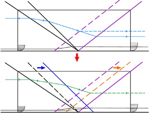
Previous studies of ISWTBLIs mostly focused on the interactions induced by a single incident shock wave (ISW). In reality, the interactions between a TBL and multiple ISWs are frequently encountered in supersonic and hypersonic flights. Studies of supersonic mixed-compression inlets (Tan, Sun & Huang Reference Tan, Sun and Huang2012; Huang et al. Reference Huang, Tan, Sun and Ling2016) showed that cowl shock and downstream surface-deflection-induced shock successively impinge the ramp-side TBL and induce a quadrangular separation with a complicated accompanying wave system (figure 1). Furthermore, the complex reflected oblique shock waves in the isolator of a supersonic inlet can also induce interactions between multiple ISWs and TBL (Huang et al. Reference Huang, Tan, Sun and Sheng2017; Li et al. Reference Li, Chang, Xu, Yu, Bao and Song2018; Wang et al. Reference Wang, Chang, Hou and Yu2020). Recently, experimental studies of dual-incident SWTBLIs (dual-ISWTBLIs) indicated that the distance between two ISWs significantly affects the separation configuration (Li et al. Reference Li, Tan, Zhang, Huang, Guo and Lin2020, Reference Li, Zhang, Tan, Jin and Li2022). These studies reported that the dual-ISWTBLIs have three typical flow patterns. In the first type of dual-ISWTBLI (type 1 dual-ISWTBLI) when the distance between two ISW impingement points was zero, the interaction was in a strong-coupling state with a triangular separation region; additionally, the flow features, such as the pressure distribution and wall-surface topology, are almost the same as those in single-incident SWTBLI (single-ISWTBLI) with identical total deflection angle. As the shock wave distance reached a moderate value, the interactions exhibited a weak-coupling state with a quadrangular separation region, which was defined as the second type of dual-ISWTBLI (type 2 dual-ISWTBLI). In the third type of dual-ISWTBLI (type 3 dual-ISWTBLI), the interactions induced by the two ISWs decoupled due to the sufficiently large shock wave distance, and the overall flow can be viewed as two individual single-ISWTBLIs. Moreover, Li et al. (Reference Li, Zhang, Tan, Jin and Li2022) provided an analysis of the separation length scaling for type 1 dual-ISWTBLIs. Based on the re-established normalised parameters, the datasets of type 1 dual-ISWTBLIs can fall close to the trend line reported in a study of single-ISWTBLIs and CRSWTBLIs by Souverein et al. (Reference Souverein, Bakker and Dupont2013).

Figure 1. Schematic of dual-ISWTBLs in a supersonic mix-compression inlet.
In a previous study, Li et al. (Reference Li, Zhang, Tan, Jin and Li2022) qualitatively obtained that the shock wave distance and the setting of the two deflection angles are crucial factors affecting the separation length in dual-ISWTBLIs; however, quantitative relations between the separation length and the influencing factors are unavailable in that study. This paper is a sequel of the study of Li et al. (Reference Li, Zhang, Tan, Jin and Li2022). In the current study, we experimentally examine two groups of dual-ISWTBLIs with two deflection angles of (7 $^\circ$, 5 $^\circ$) and (5 $^\circ$, 7 $^\circ$); for each group, five experiments are conducted to quantitatively investigate the effect of shock wave distance on the separation length. Moreover, referring to the scaling method of Souverein et al. (Reference Souverein, Bakker and Dupont2013), we conduct a control volume analysis of the mass and momentum conservations for dual-ISWTBLIs under inviscid and viscous conditions and derive the dependence of the separation length on the shock wave distance and the aerodynamic parameters for dual-ISWTBLIs with coupling separation region (i.e. type 1 and type 2 dual-ISWTBLIs).
2. Experimental methodology
2.1. Wind tunnel and test model
The experiments were performed in the supersonic wind tunnel at Nanjing University of Aeronautics and Astronautics, which is a free-jet type operating in an air-breathing mode. A Laval nozzle with a  $200\,{\rm mm} \times 200$ mm square exit was employed to produce a supersonic airflow with a free-stream Mach number of 2.73. The usable runtime of the facility is over 14 s. The free-stream stagnation pressure of the supersonic airflow was $P^* = 102 \pm 0.3$ kPa, the stagnation temperature was $T^* = 286 \pm 1.5$ K and the unit Reynolds number was $Re_{unit} = 9.2 \times 10^{6}$ m $^{-1}$. The test model is the same as that in Li et al. (Reference Li, Zhang, Tan, Jin and Li2022), as depicted in figure 2. The shock generator (SG) had a double-wedge configuration to induce two ISWs. The two sidewalls were embedded with K9 optical glass to provide optical monitoring access to the interaction region. The spanwise width of the test section was 140 mm. The sidewall leading edge was set 90 mm downstream of the bottom-wall leading edge, and this short sidewall arrangement was to afford a thin sidewall boundary layer. To ensure that the boundary layer upstream of the interaction region was fully turbulent, a transition band was implanted on the bottom wall, 10 mm downstream of the leading edge. The boundary layer developed along the bottom wall, which is under an approximately adiabatic condition (the wall temperature $T_w$ is approximately equal to the adiabatic recovery wall temperature $T_{aw}$). The flow characteristics of the boundary layer were measured at a position 195 mm downstream of the leading edge. Figure 3 depicts the TBL velocity profile. The TBL thickness was $\delta _0 = 5.90$ mm, displacement thickness was $\delta ^* = 1.94$ mm, momentum thickness was $\theta = 0.44$ mm, shape factor was $H = 4.41$ and momentum-thickness-based Reynolds number was $Re_{\theta } = 4030$. Further details of the measurement of TBL parameters are provided in Li et al. (Reference Li, Zhang, Tan, Jin and Li2022).

Figure 2. (a) Test model in the wind tunnel. (b,c) Schematics of the test model and SG. (d) Schematic of the control mechanism for rotating the SG.

Figure 3. Velocity profile of the TBL. Data from Wu & Martin (Reference Wu and Martin2007), Bookey, Wyckham & Smits (Reference Bookey, Wyckham and Smits2005) and Brooks et al. (Reference Brooks, Gupta, Smith and Marineau2015) are displayed for comparison.
Figure 2(c) depicts a schematic of the double-wedge SG. In this figure,  $O_1$ and $O_2$ are the two impingement points of the two ISWs on the bottom-wall centreline. The distance between $O_1$ and $O_2$ is defined as the shock wave distance $d$ (
$d$ ( $d = x_{O2} - x_{O1}$). Ten SGs were employed in the experiments, and table 1 presents the specific geometric parameters of the SGs. Parameter $h$ denotes the leading-edge height. Angles $\alpha _1$ and $\alpha _2$ are the two deflection angles. Lengths $l_1$ and $l_2$ are the first and second ramp lengths. The pre-tests indicated that under an identical total deflection angle of 12 $^{\circ }$, for cases with a relatively large $\alpha _2$ ( $\alpha _2 = 9^{\circ }$), a laminar boundary layer separation may occur at the corner between the first and second ramps of the SG; additionally, for cases with a relatively large $\alpha _1$ ( $\alpha _1 = 9^{\circ }$), the contraction ratio of the test channel in situations with large shock wave distances is considerable, which results in the unstart of the test channel and the wind tunnel. Therefore, within the working range of the wind tunnel, two moderate deflection angle combinations, ( $\alpha _1 = 7^{\circ }$, $\alpha _2 = 5^{\circ }$) and ( $\alpha _1 = 5^{\circ }$, $\alpha _2 = 7^{\circ }$), are selected herein to explore their effect on the separation length. The ten cases are divided into two groups according to the deflection angles: group 1 with $\alpha _1 = 7^{\circ }$ and $\alpha _2 = 5^{\circ }$ comprises cases A–E with $d = 0$, 9.5, 19.0, 28.5 and 38.0 mm, respectively; and group 2 with $\alpha _1 = 5^{\circ }$ and $\alpha _2 = 7^{\circ }$ comprises cases F–J with $d = 1.7$, 12.1, 22.5, 32.9 and 43.4 mm, respectively. The change of $d$ in each group was realised by adjusting $l_1$. The coordinate system origin is at $O_1$, which is 265 mm downstream of the bottom-wall leading edge, and the streamwise, perpendicular and spanwise directions are denoted by the $x$,
$x$,  $y$ and $z$ axes, respectively (figure 2c).
Table 1. Geometric parameters of the SGs.

It should be noted here that in the experimental study of ISWTBLIs, the impingement of the expansion waves stemming from the SG terminal on the bottom-wall boundary layer was inevitable due to the geometry limitation (Daub, Willems & Gülhan Reference Daub, Willems and Gülhan2016; Grossman & Bruce Reference Grossman and Bruce2018). In the current study, the lengths of the second ramps of the SGs were set as long as possible to ensure that the expansion-wave impingement was as far away from the SWTBLI region as possible. In all ten cases considered in the current study, the distance between the second shock impingement point and the expansion-wave impingement point is about 33 mm. However, the pre-tests showed that under the condition of the relatively long SGs, if the total deflection angle of the SG was set to the target value of 12 $^{\circ }$ before the test, the test channel could not self-start due to a relatively large contraction ratio. Therefore, we adopted a method of rotating the SG to ensure that the supersonic interaction flow could be successfully established under the geometric conditions of a relatively long SG: before the test, the total deflection angle of the SG was set to a relatively small angle (less than 8 $^{\circ }$) to ensure the self-start of the test channel; after the supersonic flow was successfully formed in the test channel, the SG was rotated to the target position (total deflection angle is 12 $^{\circ }$) by a control mechanism, which consists of a series of connecting rods and a step motor (shown in figure 2d). In addition, we also tried to use a longer SG to ensure the distance between the second shock impingement point and the expansion-wave impingement point was about 36 mm; however, in some conditions with large shock wave distances, the pre-tests showed that the wind tunnel could only self-start when the total deflection angle was small, but the test channel fell into an unstart status after the SG was rotated to the target position. This phenomenon indicated that under the current experimental conditions, the lengths of the SGs shown in table 1 were close to the limit values for ensuring the start of the test channel.
2.2. Measurement technique
This study employed schlieren photography, oil-flow visualisation and static pressure measurements to diagnose the flow features in dual-ISWTBLIs, and these techniques have been reported in Li et al. (Reference Li, Zhang, Tan, Jin and Li2022). Herein, we briefly introduce these techniques for the sake of completeness. A Z-type schlieren system was employed to visualise the flow configurations in the  $x$–
$x$– $y$ plane, which comprises a xenon lamp, two concave mirrors and a horizontally placed knife edge. The schlieren images with $1000 \times 400$ resolution ( $\approx$7 pixels mm $^{-1}$) were recorded using a NAC HX-3 high-speed camera at an 8 k frame rate. The oil-flow visualisation was performed on the bottom wall. The oil-flow mixture, consisting of white silicon dioxide (SiO ${_2}$) powder, oleic acid and dimethylsilicone, was evenly applied to the bottom-wall surface before each test. Live image sequences were recorded with a Canon EOS-1D X Mark II digital camera during the wind tunnel operation. The resolution of the captured oil-flow images is $5742 \times 3648$ ( $\approx$12 pixels mm $^{-1}$). Additionally, to measure the wall-pressure distribution on the bottom wall, 55 pressure taps with a 3 mm spacing were set on the centreline, in the streamwise range of 165–327 mm from the leading edge (figure 2b). CYG-503 transducers with a 100 kPa measurement range and a 0.1 % full-scale accuracy (i.e. $\pm$0.1 kPa) were used as sensor elements, and the pressure signals were collected by two DAQ-PCI-6225 cards (National Instruments) at a 1 kHz sampling rate.
3. Experimental results
Li et al. (Reference Li, Zhang, Tan, Jin and Li2022) reported that when the first ISW was fixed, the separation point of the dual-ISWTBLIs moved downstream with increasing  $d$, and the separation height concurrently decreased. These features are also reflected in the schlieren images obtained in this study (figure 4). In figure 4, the yellow dashed line represents the outline of the shear layer; the yellow and green dots represent the spanwise-averaged locations of the separation and reattachment points, respectively (obtained from the oil-flow images); the blue dashed-dotted lines represent the height of the separation bubble (obtained according to the outline of the shear layer); the purple dashed lines denote the position of the first ISW impingement point; and the cyan dashed line indicates the change of streamwise position of the second ISW impingement point in different cases. As is known, dual-ISWTBLIs possess more complex wave structures than single-ISWTBLIs (Li et al. Reference Li, Zhang, Tan, Jin and Li2022). Previous studies of single-ISWTBLIs reveal that the ISW impingement on the shear layer of the separation region induces a centred expansion fan emanating from the apex of the separation (Babinsky & Harvey Reference Babinsky and Harvey2011). For dual-ISWTBLIs, the impingements of the two ISWs on the shear layer lead to two expansion fans. Figure 4 shows that when $d$ tends to zero (type 1 dual-ISWTBLI), the two impingement points of ISWs on the shear layer are very close; thus, the two expansion fans merge into one, after which the main flow turns to the wall, and the separation in this situation exhibits a triangular shape (case A). As $d$ increases, the two expansion fans decouple. The two reflections of the ISWs deflect the main flow twice, and the overall flow exhibits a quadrangular separation, yielding type 2 dual-ISWTBLIs (cases B–D and cases G–I). Cases E and J correspond to type 3 dual-ISWTBLIs, wherein the values of $d$ are sufficiently large, so the sub-interactions induced by the two ISWs decouple; in other words, the overall flow consists of two isolated single-ISWTBLIs in this situation. Figures 5(a) and 5(b) display the static pressure distributions along the wall centrelines of group 1 and group 2, respectively, which also indicate that the onset of pressure rise moves downstream with increasing $d$. Figure 5(c) shows the pressure distributions for cases E and J (type 3 dual-ISWTBLIs), and the dashed-dotted lines represent the inviscid pressure rise for the two cases. Closer inspection indicates that the pressure distribution in type 3 dual-ISWTBLIs exhibits two pressure-rise stages corresponding to the two isolated single-ISWTBLIs. Note that the pressure drop occurring after the apex of the pressure curves in cases A–D and F–H is caused by the impingement of the expansion fan stemming from the SG terminal; this phenomenon is inevitable in the experimental studies of ISWTBLIs due to the geometric constraint of the test model, even though the lengths of the SGs were set as long as possible in this paper.

Figure 4. Schlieren images. Panels (a–j) correspond to cases A–J, respectively. Yellow and green dots represent the separation and reattachment points, respectively, obtained from the oil-flow images. The purple dashed lines indicate the position of the impingement point of the first ISW. The cyan dashed line indicates the change of streamwise position of the second ISW impingement point in different cases.

Figure 5. Pressure distribution along the bottom-wall centreline. (a) Cases A–E. (b) Cases F–J. (c) Cases E and J (type 3 dual-ISWTBLIs). (d) Initial pressure rises during the free interaction for cases A–D and F–I (the pressure rises of cases B–D and F–I are aligned with that of case A).
For type 2 dual-ISWTBLIs with a quadrangular separation, the shear layer of the separation bubble was split into three parts by the two impingement points of the ISWs on the shear layer. The schlieren images in figure 4 show that the flow directions of the shear layer between the two impingement points in the two groups of type 2 dual-ISWTBLIs (i.e. cases B–D and cases G–I) are slightly downward and slightly upward, respectively, and the flow directions of these shear layers in each group are independent of  $d$. Li et al. (Reference Li, Zhang, Tan, Jin and Li2022) reported that the quadrangular separation bubble in type 2 dual-ISWTBLIs has three different shapes, and the difference is reflected in the flow direction of the shear layer between the two impingement points of the ISWs on the shear layer. Figure 6 displays schematics of the three types of quadrangular separations, in which the three parts of the shear layer are simplified to $S$–
$S$– $T_1$, $T_1$– $T_2$ and $T_2$– $R$ (
$R$ ( $S$ and $R$ represent the separation and reattachment points, respectively; $T_1$ and $T_2$ represent the two impingement points of the ISWs on the shear layer). Based on an inviscid model, Li et al. (Reference Li, Zhang, Tan, Jin and Li2022) found that the flow direction of $T_1$– $T_2$ depends only on the first deflection angle $\alpha _1$ and the deflection angle $\alpha _3$ at the separation point. A critical value of the first deflection angle $\alpha _{1cr}\approx 0.5\alpha _3$ exists under the conditions of $1.0 < Ma_0 < 7.0$ and $0^{\circ } < \alpha _3 < 14.0^{\circ }$ ( $Ma_0$ represents the incoming free-stream Mach number): when $\alpha _{1} < \alpha _{1cr}$, the shear layer $T_1$– $T_2$ is upward and $T_2$ is the apex of the separation bubble; when $\alpha _{1} = \alpha _{1cr}$, $T_1$– $T_2$ is parallel to the bottom wall; and when $\alpha _{1} > \alpha _{1cr}$, $T_1$– $T_2$ is downward and $T_1$ is the apex of the separation bubble. For the large-scale separation in cases A–D and F–I, the pressure plateau is approximately constant, and the pressure rises in these cases before reaching the plateau pressure $p_p$ are approximately superposable (shown in figure 5d), which is consistent with the free interaction theory of Chapman et al. (Reference Chapman, Kuehn and Larson1957). The deflection angle $\alpha _3$ at the separation can be estimated through the plateau pressure $p_p$ (Matheis & Hickel Reference Matheis and Hickel2015; Li et al. Reference Li, Zhang, Tan, Jin and Li2022):
 \begin{equation} \alpha_{3}=\arctan \left[\frac{({p_p}/{p_0}-1)^{2} \left[2 \gamma\left(Ma_{0}^{2}-1\right)-(\gamma+1) ({p_p}/{p_0}-1)\right]}{\left[\gamma Ma_{0}^{2}-({p_p}/{p_0}-1)\right]^{2} [2 \gamma+(\gamma+1)({p_p}/{p_0}-1)]}\right]^{0.5}. \end{equation}
Figure 6. (a–c) Schematics of three types of quadrangular separation.
Figure 4(d) shows that  $p_p$/ $p_0\approx 2.29$; thus $\alpha _{3}\approx 12.6^{\circ }$ and $\alpha _{1cr}\approx 6.3^{\circ }$ in this study. For cases B–D, $\alpha _{1} = 7^{\circ } > \alpha _{1cr}$, while $\alpha _{1} = 5^{\circ } < \alpha _{1cr}$ for cases G–I; thus the flow direction of the shear layer between the two impingement points ( $T_1$ and $T_2$) in cases B–D and cases G–I is slightly downward and upward, respectively.
In previous literature, the numerical simulations generally focus on quasi-two-dimensional ISWTBLIs by assuming spanwise homogeneity for simplicity (Pirozzoli & Grasso Reference Pirozzoli and Grasso2006; Priebe, Wu & Martin Reference Priebe, Wu and Martin2009; Pirozzoli & Bernardini Reference Pirozzoli and Bernardini2011; Tong et al. Reference Tong, Li, Yuan and Yu2020). In fact, typical quasi-two-dimensional interactions only exist within a limited spanwise region in experimental studies, because the ISW interacts with the sidewall boundary layer and induces complex three-dimensional corner flows in the junction of the bottom and side walls (Green Reference Green1970; Reda & Murphy Reference Reda and Murphy1973; Bookey et al. Reference Bookey, Wyckham and Smits2005; Humble et al. Reference Humble, Elsinga, Scarano and Van Oudheusden2009a; Humble, Scarano & Van Oudheusden Reference Humble, Scarano and Van Oudheusden2009b; Babinsky, Oorebeek & Cottingham Reference Babinsky, Oorebeek and Cottingham2013; Benek, Suchyta & Babinsky Reference Benek, Suchyta and Babinsky2014; Bermejo-Moreno et al. Reference Bermejo-Moreno, Campo, Larsson, Bodart, Helmer and Eaton2014; Wang et al. Reference Wang, Sandham, Hu and Liu2015; Grossman & Bruce Reference Grossman and Bruce2018; Xiang & Babinsky Reference Xiang and Babinsky2019). In this paper, a short sidewall is used to restrict the thickness of the sidewall boundary layer to reduce the influence region of the sidewall effect. Nevertheless, the sidewall effect cannot be completely eliminated. Figures 7 and 8 show the oil-flow topologies for cases A–J, where the separation and reattachment lines are indicated by the red and cyan lines, respectively. Due to the influence of the sidewall effect, the overall separation exhibits three-dimensional features, and the separation and reattachment lines are curved along the spanwise direction. Comparison of the curvature of the separation and reattachment lines shows that the effect of the three-dimensional separated flows on the reattachment line is stronger than that on the separation line, this phenomenon also being reported by Grossman & Bruce (Reference Grossman and Bruce2018). The locations of the separation and reattachment lines are averaged along the spanwise direction, which are marked in figures 7 and 8 by yellow and green dashed lines, respectively. The topologies for all the cases are almost symmetric about the bottom-wall centreline. For the interactions that present a coupling separation state (i.e. cases A–D and F–I), the surface topologies are similar, and case F is taken as an example herein to briefly introduce the distribution of the critical points in the oil-flow topologies. As shown in figures 9(a) and 9(b), both the separation and reattachment lines present ‘saddle–node–saddle’ configurations, i.e.  $S_1$– $N_1$– $S_1'$ and $S_2$– $N_2$– $S_2'$. Two focus points, $F_1$ and $F_1'$, exist near the junction corners of the bottom and side walls. Moreover, two saddle points ( $S_3$ and $S_4$) and two focus points ( $F_2$ and $F_2'$) are present in the region between $N_1$ and $N_2$ (see Li et al. (Reference Li, Zhang, Tan, Jin and Li2022) for more details of this type of critical-point distribution in the surface topology). For cases A–D and F–I, the two lines connecting the two groups of saddle points (i.e. lines $S_1$– $S_2$ and $S_1'$– $S_2'$) divide the overall flow region into three parts, namely the central core-flow region and two sidewall-influence regions.

Figure 7. Oil-flow images for group 1. Panels (a–e) correspond to cases A–E, respectively. The red and cyan lines represent the separation and reattachment lines, respectively. The white dashed line indicates the streamwise location of the first shock impingement point. The yellow and green dashed lines indicate the spanwise-averaged position of the separation and reattachment lines, respectively. The blue dots represent the two saddle points on the reattachment line.

Figure 8. Oil-flow images for group 2. Panels (a–e) correspond to cases F–J, respectively. The red and cyan lines represent the separation and reattachment lines, respectively. The white dashed line indicates the streamwise location of the first shock impingement point. The yellow and green dashed lines indicate the spanwise-averaged position of the separation and reattachment lines, respectively. The blue dots represent the two saddle points on the reattachment line.

Figure 9. Surface topologies of cases F and J. (a) Oil-flow image and (b) corresponding annotated diagram for case F. (c) Oil-flow image and (d) corresponding annotated diagram for case J. The red dashed line represents the centrelines in (b,d).
For type 3 dual-ISWTBLs in cases E and J, the surface topologies are evidently different from those in the type 1 and type 2 dual-ISWTBLIs. In case E, only the separation and reattachment lines of the incipient separation caused by the first ISW can be recognised; however, no apparent separation and reattachment lines of the sub-interaction induced by the second ISW can be detected from the oil-flow images because the interaction strength is relatively weak. By comparison, there are two separation regions in case J, and the surface topology is relatively complicated: as shown in figures 9(c) and 9(d), the first separation region is relatively small, bounded by the separation and reattachment lines with weak bending along the spanwise direction; however, the separation region induced by the second single-ISWTBLI possesses strong three-dimensional characteristics, which are caused by the sidewall effect and the spanwise inhomogeneity of the boundary layer downstream of the first single-ISWTBLI. In the second separation region of case J, there are two visible focus points ( $F_1$ and $F_1'$) near the centreline and one reattachment node ( $N_1$) in the centre of the reattachment line. One interesting phenomenon is that in the central part of the second single-ISWTBLI region, the oil traces near the centreline maintain a forward direction in a relatively large streamwise range, and the separation line is very close to the reattachment line in this region. Based on the flow direction of the oil trace, we can infer that there should be a saddle point ( $S_3$) upstream of $N_1$ to ensure the consistency of the surface topology, although this saddle point cannot be clearly observed in the oil-flow image; at the saddle point $S_3$, the streamlines from the upstream region move to both sides and finally spiral into the two focus points $F_1$ and $F_1'$. In addition, there are a pair of separation saddle points ( $S_1$ and $S_1'$) and a pair of reattachment saddle points ( $S_2$ and $S_2'$) in the region between the centreline and the sidewalls in case J, and the distributions of these two pairs of saddle points are similar to those in the surface topology of single-ISWTBLIs reported by Li et al. (Reference Li, Zhang, Tan, Jin and Li2022).
To quantitatively compare the difference in separation length among the ten cases, the parameters of the separation region are extracted from the schlieren and oil-flow images, listed in table 2. Positions  $x_S$ and $x_R$ denote the spanwise-averaged positions of the separation and reattachment lines, respectively. Length $L_{{sep}} = {x_R} - {x_S}$ represents the overall separation length and $L_{{int}} = {x_{O1}} - {x_{S}}$ represents the upstream interaction length. Additionally, $h_{{sep}}$ is the height of the separation region, which is roughly obtained based on the outline of the shear layer (the yellow dashed line in the schlieren images in figure 4). Figure 10(a) plots the curves of $L_{{sep}}$ versus $d$, depicting $L_{{sep}}$ first increasing and then decreasing with $d$. Figures 10(b) and 10(c) show that $L_{{int}}$ and $h_{{sep}}$ decrease with increasing $d$. In reality, for the cases with coupling separations in both groups of interactions (i.e. cases A–D and F–I), $L_{{sep}}$ changes little with $d$; the maximum relative deviation of $L_{{sep}}$ for cases A–D is 6.1 % and for cases F–I is 5.9 %. When the flow pattern changes to the decoupling state, $L_{{int}}$ and $L_{{sep}}$ decrease sharply. Note that the $L_{{sep}}$ value for case E represents the separation length of the first single-ISWTBLI since no visible separation region for the second single-ISWTBLI can be identified from the oil-flow images in this case, while the $L_{{sep}}$ value for case J represents the total separation length of the first and second single-ISWTBLIs. Careful inspection of figure 10(b) indicates that $L_{{int}}$ approximately linearly decreases with increasing $d$ for the cases with a coupling separation. The two linear regressions for the variations of $L_{{int}}$ versus $d$ for cases A–D and F–I are shown in figure 10(b) as black and purple dashed-dotted lines with slopes of $-0.647$ and $-0.797$, respectively, indicating that the decrease rate of $L_{{int}}$ versus $d$ is greater in group 2 than that in group 1. As shown in § 2.1, the difference between the experimental settings of the two groups of interactions is reflected in the deflection angles, which means that the deflection angle combination is a key influencing factor in the upstream interaction length of the separation. Furthermore, the spanwise width of the core flow ( $W_{{cf}}$) in the central region of the test section is obtained based on the spanwise distance between the two saddles on the reattachment line (i.e. $S_2$ and $S_2'$, marked by the blue dots in the oil-flow images in figures 7 and 8). The curves of $W_{{cf}}$ versus $d$ for the interactions with a coupling separation are plotted in figure 10(d), which show that the $W_{{cf}}$ values for cases A–D are 67.7, 67.1, 69.1 and 68.4 mm, respectively, and for cases F–I are 67.0, 71.0, 68.3 and 68.7 mm, respectively. In fact, the spanwise extent of the core flow is an important parameter for the design of the supersonic inlet. It is known that the air quality at the exit section of the supersonic inlet is significant for the performance of the engine. However, the complex corner flow induced by the sidewall effect generally has a negative impact on the total pressure recovery and distortion of the airflow. In comparison, the quality of the core flow in the central region is relatively high, which signifies that the larger the width of the central core-flow region, the higher the air quality of the exit section of the inlet. The experimental results shown in figure 10(d) indicate that $W_{{cf}}$ changes little with $d$ and the deflection angle combinations under the experimental conditions considered in the current study, which can provide a certain reference for the practical engineering design of the supersonic inlet.

Figure 10. Effect of shock wave distance on (a) separation length  $L_{sep}$, (b) upstream interaction length $L_{int}$, (c) separation height $h_{{sep}}$ and (d) spanwise width of the central core flow $W_{{cf}}$.
Table 2. Parameters of separation region in cases A–J.

In case J, the superscript  $^{*}$ represents the streamwise positions of the separation and reattachment points for the second single-ISWTBLI, and the superscript ${\dagger}$ represents the total separation length of the first and second single-ISWTBLIs.
4. Separation length scaling for dual-ISWTBLIs
The above experimental results demonstrate that the separation length is dependent on shock wave distance and the deflection angles. Here, it should be noted that once the interaction flow is decoupled into two single-ISWTBLIs (i.e. forming type 3 dual-ISWTBLI), we can think that the separation lengths of the two sub-interactions are no longer affected by  $d$, and they can be estimated roughly by the length scaling methods of single-ISWTBLIs. Consequently, this section mainly focuses on the separation length scaling for type 1 and type 2 dual-ISWTBLIs, and the relation between the separation length and the influencing factors is analytically investigated by referring to the scaling method in Souverein et al. (Reference Souverein, Bakker and Dupont2013).
In the study of Souverein et al. (Reference Souverein, Bakker and Dupont2013), the normalised interaction length  $L^*$ was proposed for single-ISWTBLIs and CRSWTBLIs based on a control volume analysis of mass conservation. Using the new interaction strength metric $S_e^*$, the normalised interaction length $L^*$ for the single-ISWTBLIs and CRSWTBLIs obtained from the datasets in the literature can fall close to a single trend line with a moderate scatter. In the recent experimental study, some flow features, such as the separation shape and pressure rise, for type I dual-ISWTBLIs were observed nearly the same as those for single-ISWTBLIs under an identical total deflection angle condition; thus, Li et al. (Reference Li, Zhang, Tan, Jin and Li2022) conducted a similar control volume analysis for type 1 dual-ISWTBLIs and established new normalised interaction length $L_{{dual}}^{*}$ and normalised interaction strength $S_{{e,dual}}^{*}$, by which the separation lengths for type 1 dual-ISWTBLIs and single-ISWTBLIs can be reconciled. The experimental results in § 3 show that both shock wave distance $d$ and the deflection angles affect the interaction length of the separation region. However, the effect of $d$ is not reflected in the normalised parameters $L_{{dual}}^{*}$ and $S_{{e,dual}}^{*}$ for type I dual-ISWTBLI in Li et al. (Reference Li, Zhang, Tan, Jin and Li2022), indicating that the two normalised parameters are no longer applicable to the separation length scaling for dual-ISWTBLIs with $d > 0$. Therefore, in analogy with the method in Souverein et al. (Reference Souverein, Bakker and Dupont2013), control volume analysis of both mass and momentum conservations is performed for type 1 and type 2 dual-ISWTBLIs in this section, and the differences in the mass and momentum fluxes between the two types of dual-ISWTBLIs are studied to determine the effect of $d$ on the separation length. The control volume analysis of type 1 dual-ISWTBLIs was reported in Li et al. (Reference Li, Zhang, Tan, Jin and Li2022); herein, we reintroduce it briefly for the sake of completeness.
Figure 11 shows the control volume for type 1 dual-ISWTBLIs. In this figure,  $L_{{cv}}$ and $h_{{cv}}$ are the length and height of the control volume, respectively. Compared with the control volume for single-ISWTBLIs in Souverein et al. (Reference Souverein, Bakker and Dupont2013), $L_{{cv}}$ in type 1 dual-ISWTBLIs is split into two parts (i.e. $L_1$ and $L_2$) by the second ISW. Under the inviscid condition, the two ISWs intersect at the wall, and the reflected shock wave (RSW; shown as the purple solid line in figure 11) originates from the intersection. Under the viscous condition, the displacement thickness $\delta ^{*}$ and momentum thickness $\theta$ are used to model the TBL presence. As described by Souverein et al. (Reference Souverein, Bakker and Dupont2013), the SWTBLI region can be regarded as a black box that modifies the mass and momentum fluxes within the TBL; the only way to ensure mass balance and momentum balance in the control volume under the viscous condition is to translate the RSW upstream to form the translated RSW (TRSW; shown as the purple dashed line in figure 11), which can be regarded as the separation-induced shock wave in ISWTBLIs. In figure 11, $L_{{int},0}$ can be regarded as the upstream interaction length for type 1 dual-ISWTBLIs with $d = 0$. Herein, some basic assumptions similar to those in Souverein et al. (Reference Souverein, Bakker and Dupont2013) are adopted: TRSW is parallel to RSW, which satisfies a perfect-fluid reflection of an oblique shock wave; the flow conditions in the region outside the boundary layer are uniform and approach the perfect-fluid solutions calculated through the inviscid shock relations; and the incoming and outgoing boundary layers are in a fully turbulent state.

Figure 11. Control volume for type 1 dual-ISWTBLIs.
According to the control volume in figure 11, the mass conservation under the inviscid condition satisfies
 \begin{equation} {{\rho}_{{0}}}{{u}_{{0}}}{{h}_{cv}}+{{\rho }_{{1}}}{{v}_{{1}}}{{L}_{{1}}}+ {{\rho }_{{2}}}{{v}_{{2}}}{{L}_{{2}}}-{{\rho }_{{3}}}{{u}_{{3}}}{{h}_{cv}}=0 \end{equation}
and the mass balance under viscous conditions can be expressed by
 \begin{equation} {{\rho }_{{0}}}{{u}_{{0}}}\left( {{h}_{cv}}-\delta _{{0}}^{*} \right)+ {{\rho }_{{1}}}{{v}_{{1}}}{{L}_{{1}}}+{{\rho }_{{2}}}{{v}_{{2}}} \left( {{L}_{{2}}}-L_{{int},0} \right)-{{\rho }_{{3}}}{{u}_{{3}}} \left( {{h}_{cv}}-\delta _{{3}}^{*} \right)=0, \end{equation}
where  $\rho _{i}$ is the density, $u_i$ and $v_i$ are the $x$- and $y$-direction components of velocity, respectively, and $\delta _{0}^{*}$ and $\delta _{3}^{*}$ are the displacement thicknesses for the incoming and outgoing TBL, respectively. The subscripts $i = 0$, 1, 2 and 3 denote the parameters in the flow regions (0)–(3) in figure 11.
Subtracting (4.2) from (4.1) yields
 \begin{equation} L_{{int},0}=\frac{{{\rho }_{{3}}}{{u}_{{3}}}\delta _{3}^{*}-{{\rho }_{{0}}}{{u}_{{0}}} \delta _{{0}}^{*}}{{{\rho }_{{2}}}{{v}_{{2}}}}= \frac{\sin \left( {{\beta }_{1}}-{{\alpha }_{1}} \right)\sin \left( {{\beta }_{2}}-{{\alpha }_{2}} \right)}{\sin \left( {{\beta }_{1}} \right)\sin \left( {{\beta }_{2}} \right)\sin \left( {{\alpha }_{1}}+{{\alpha }_{2}} \right)} \left(\frac{{{\rho }_{{3}}}{{u}_{{3}}}\delta _{{3}}^{*}}{{{\rho }_{{0}}}{{u}_{{0}}} \delta _{{0}}^{*}}-1 \right)\delta _{{0}}^{*}, \end{equation}
where  $\alpha _1$ and $\alpha _2$ are the first and second deflection angles, respectively, and $\beta _1$ and $\beta _2$ are the first and second shock angles, respectively. We define the mass-flow deficit as $\dot {m} = {\rho }u{\delta ^{*}}$ and rewrite (4.3) as
 \begin{equation} \frac{L_{{int},0}}{\delta_{in}^{*}}=g\left( M{{a}_{{0}}},{{\alpha }_{1}},{{\alpha }_{2}} \right) \left( \frac{\dot{m}_{out}^{*}}{\dot{m}_{in}^{*}}-1 \right), \end{equation}
where the subscripts  ${in}$ and ${out}$ represent the parameters for incoming and outgoing TBL and $g({Ma_0}, {\alpha _1},{\alpha _2})$ is a sine function related to the test model geometry:
 \begin{equation} {{g}}\left( M{{a}_{0}},{{\alpha }_{{1}}},{{\alpha }_{{2}}} \right)= \frac{\sin \left( {{\beta }_{1}}-{{\alpha }_{1}} \right)\sin \left( {{\beta }_{2}}-{{\alpha }_{2}} \right)}{\sin \left( {{\beta }_{1}} \right)\sin \left( {{\beta }_{2}} \right)\sin \left( {{\alpha }_{1}}+{{\alpha }_{2}} \right)}. \end{equation}
 In analogy with the definition in Souverein et al. (Reference Souverein, Bakker and Dupont2013), the interaction length for type 1 dual-ISWTBLI is normalised by the TBL displacement thickness  $\delta _{in}^{*}$ and the sine function $g({Ma_0}, {\alpha _1},{\alpha _2})$, i.e. the normalised interaction length for type 1 dual-ISWTBLI is
 \begin{equation} {{L}^{{*}}_{dual}}=\frac{L_{{int},0}}{\delta_{in}^{*}g\left( M{{a}_{0}},{{\alpha }_{{1}}}, {{\alpha }_{{2}}} \right)}= \frac{\dot{m}_{out}^{*}}{\dot{m}_{in}^{*}}-1 \end{equation}
and the normalised interaction strength metric is defined as
 \begin{equation} S_{e,dual}^{*}=\frac{2k}{\gamma} \frac{\displaystyle\frac{p_{{post}}}{p_{{pre}}}-1}{Ma_{0}^{2}},\quad k=\left\{\begin{array}{@{}ll} 3.0, & \text{if}\ {Re}_{\theta}\leq1\times10^{4},\\ 2.5, & \text{if}\ {Re}_{\theta}>1\times10^{4}, \end{array}\right. \end{equation}
where  $p_{{pre}}$ and $p_{{post}}$ are the pressures before and after the interaction region, respectively, and $k$ is an empirical constant, which is related to $Re_{\theta }$. The experimental results in Li et al. (Reference Li, Zhang, Tan, Jin and Li2022) showed that $L_{{dual}}^{*}$ and $S_{{e,dual}}^{*}$ for type I dual-ISWTBLIs can fall close to the trend line $L^{*} = 1.3 \times (S_{e}^{*})^3$ proposed for single-ISWTBLIs and CRSWTBLIs in Souverein et al. (Reference Souverein, Bakker and Dupont2013).
The experimental results in § 3 show that when the first ISW is fixed,  ${L_{{int}}}$ nearly linearly decreases with increasing $d$. Figure 12 shows the control volume for dual-ISWTBLIs with $d > 0$. In figure 12, the second ISW and TRSW for type 2 dual-ISWTBLIs are shown as the blue solid and orange dashed lines, respectively, and the second ISW and TRSW for type 1 dual-ISWTBLIs are shown as black and purple dashed lines for comparison. Length ${L_{{int},d}}$ represents the upstream interaction length for type 2 dual-ISWTBLIs with $d > 0$. Compared with the shock waves of type 1 dual-ISWTBLIs in figure 11, the second ISW moves $d$ downstream in figure 12; accordingly, the TRSW moves ${\rm \Delta} {L_{{int}}}$ downstream ( ${\rm \Delta} {L_{{int}}} = {L_{{int},0}} - {L_{{int},d}}$). For type 2 dual-ISWTBLIs, we can assume that the intensity of the TRSW is the same as that in type 1 dual-ISWTBLIs because the free interaction theory of Chapman et al. (Reference Chapman, Kuehn and Larson1957) reported that the intensity of the separation shock in a large-scale separation remains unchanged when the characteristics of the incoming TBL are identical. Thus, the flow conditions in the regions outside the boundary layer (i.e. regions (0)–(3)) can be viewed as the same as those in type 1 dual-ISWTBLIs. As described above, the RSW is translated to balance the mass and momentum deficits of the incoming and outgoing boundary layers. Compared with type 1 dual-ISWTBLIs, the change in ${L_{{int}}}$ in type 2 dual-ISWTBLIs results in a change in the characteristics of the outgoing TBL; accordingly, we define the displacement and momentum thicknesses of the outgoing TBL in type 2 dual-ISWTBLIs as ${\delta _3^*}'$ and ${\theta }'_{3}$, respectively. Note that the outgoing boundary layer is still regarded as being in a fully turbulent state, as long as the control volume is sufficiently large.

Figure 12. Control volume for type 2 dual-ISWTBLIs with  $d > 0$.
According to the control volume in figure 12, the mass conservation equation for type 2 dual-ISWTBLIs under the viscous condition satisfies
 \begin{align} & {{\rho }_{{0}}}{{u}_{{0}}}\left( {{h}_{cv}}-\delta _{{0}}^{*} \right)+ {{\rho }_{{1}}}{{v}_{{1}}}\left( {{L}_{{1}}}+d \right)+{{\rho }_{{2}}}{{v}_{{2}}} \left( {{L}_{{2}}}-{L_{{int},0}}-d+{\rm \Delta} {L_{{int}}} \right) \nonumber\\ &\quad -{{\rho }_{{3}}}{{u}_{{3}}}\left( {{h}_{cv}}-{{\delta }_{3}^{*}}' \right)=0. \end{align}
 Equations (4.2) and (4.8) present the mass balance for type 1 and type 2 dual-ISWTBLIs under the viscous condition. In fact, in the two types of dual-ISWTBLIs, the mass flows within the outgoing TBLs are different. By subtracting (4.2) from (4.8), we can get that the variation of mass flow within the outgoing TBL for the two types of dual-ISWTBLIs is related to the shock wave distance  $d$ and the change in the upstream interaction length ${\rm \Delta} {L_{{int}}}$ between the two types of dual-ISWTBLIs:
 \begin{equation} {{\rho }_{{3}}}{{u}_{{3}}}\left( \delta _{3}^{*}-{{\delta }_{3}^{*}}' \right)= {{\rho }_{{1}}}{{v}_{{1}}}d+{{\rho }_{{2}}}{{v}_{{2}}}\left( {\rm \Delta} {L_{{int}}}-d \right). \end{equation}
In analogy with the above analysis of the mass conservation, the control volume analysis of the momentum conservation is also applied to the two types of dual-ISWTBLIs. Note that the momentum deficit within the boundary layer can be obtained using the following integral equation:
 \begin{align} \int_{0}^{\infty }{\left( {{\rho }_{0}}u_{0}^{2}-\rho {{u}^{2}} \right)}{{\rm d}y} &= {{\rho }_{0}}u_{0}^{2}\int_{0}^{\infty }{\left( 1-\frac{\rho {{u}^{2}}}{{{\rho }_{0}}u_{0}^{2}} \right)}{{\rm d}y} \nonumber\\ &= {{\rho }_{0}}u_{0}^{2}\left[ \int_{0}^{\infty }{\left( 1-\frac{\rho u}{{{\rho }_{0}}{{u}_{0}}} \right)}{{\rm d}y}+ \int_{0}^{\infty }{\frac{\rho u}{{{\rho }_{0}}{{u}_{0}}}\left( 1-\frac{u}{{{u}_{0}}} \right)}{{\rm d}y} \right] \nonumber\\ &= {{\rho }_{0}}u_{0}^{2}\left( {{\delta }^{*}}+\theta \right)={{\rho }_{0}}u_{0}^{2}\theta \left( 1+H \right), \end{align}
where  $H = {\delta ^{*}}/{\theta }$ represents the shape factor.
The magnitude analysis by Souverein et al. (Reference Souverein, Bakker and Dupont2013) showed that the pressure difference force is considerably greater than the wall friction. The recent numerical studies of single-ISWTBLIs by Xie et al. (Reference Xie, Yang, Zhao, Zhang and Guo2022) also showed that the wall friction is two orders of magnitude smaller than the pressure difference force and the momentum difference of the mainstream. Therefore, in the following analysis of momentum conservation in the  $x$ direction, the influence of the wall friction on the momentum is neglected.
For type 1 dual-ISWTBLIs, the  $x$-direction momentum conservation satisfies
 \begin{align} & {{\rho }_{{0}}}u_{{0}}^{2}\left[ {{h}_{cv}}-{{\theta }_{{0}}}\left( 1+{{H}_{0}} \right) \right]+ {{\rho }_{{1}}}{{u}_{{1}}}{{v}_{{1}}}{{L}_{{1}}}+{{\rho }_{{2}}}{{u}_{{2}}}{{v}_{{2}}} \left( {{L}_{{2}}}-L_{{int},0} \right)-{{\rho }_{{3}}}u_{{3}}^{2} \left[ {{h}_{cv}}-{{\theta }_{3}}\left( 1+{{H}_{3}} \right) \right] \nonumber\\ &\quad =\left( {{p}_{{3}}}-{{p}_{{0}}} \right){{h}_{cv}}, \end{align}
where  $H_0$ and $H_3$ are the shape factors for the incoming and outgoing TBLs in type 1 dual-ISWTBLIs, respectively.
Considering the movement of the second ISW and TRSW, the  $x$-direction momentum conservation for type 2 dual-ISWTBLIs satisfies
 \begin{align} & {{\rho }_{{0}}}u_{{0}}^{2}\left[ {{h}_{cv}}-{{\theta }_{{0}}} \left( 1+{{H}_{0}} \right) \right]+{{\rho }_{{1}}}{{u}_{{1}}}{{v}_{{1}}} \left( {{L}_{{1}}}+d \right)+{{\rho }_{{2}}}{{u}_{{2}}}{{v}_{{2}}} \left( {{L}_{{2}}}-L_{{int},0}-d+{\rm \Delta} L_{{int}} \right) \nonumber\\ &\quad -{{\rho }_{{3}}}u_{{3}}^{2}\left[ {{h}_{cv}}-{{\theta }'_{3}} \left( 1+{{H}'_{3}} \right) \right]=\left( {{p}_{{3}}}-{{p}_{{0}}} \right){{h}_{cv}}, \end{align}
where  ${H'_3} = {{\delta }_{3}^{*}}' / {{\theta }'_3}$ represents the shape factor for the outgoing TBL in type 2 dual-ISWTBLIs.
In analogy with the derivation of (4.9), we subtract (4.11) from (4.12) and get that the variation of momentum flux within the outgoing TBLs between type 1 and type 2 dual-ISWTBLIs is also related to the shock wave distance  $d$ and the change in the upstream interaction length ${\rm \Delta} {L_{{int}}}$:
 \begin{equation} {{\rho }_{{3}}}u_{{3}}^{2}\left[ {{\theta }_{3}}\left( 1+{{H}_{3}} \right) -{{\theta }'_{3}} \left( 1+{{H}'_{3}} \right) \right] = {{\rho }_{{1}}}{{u}_{{1}}}{{v}_{{1}}}d+ {{\rho }_{{2}}}{{u}_{{2}}}{{v}_{{2}}}\left( {\rm \Delta} L_{{int}}-d \right). \end{equation}
 Equations (4.9) and (4.13) indicate that the relation between  ${\rm \Delta} {L_{{int}}}$ and $d$ depends on the main flow parameters and the change in outgoing TBL characteristics between the two types of dual-ISWTBLIs. Herein, we first analyse the outgoing TBL characteristics for the two types of dual-ISWTBLIs. The shape factor is a crucial parameter for the boundary layer. In reality, the shape factor $H$ is strongly related to the Mach number for compressible flow; in contrast, the incompressible shape factor $H_{{ic}}$, when neglecting the compressibility of the airflow within the boundary layer, is commonly used in the literature because $H_{{ic}}$ changes little for fully TBLs (Babinsky & Harvey Reference Babinsky and Harvey2011). For the relation between the incompressible and compressible shape factors, Cousteix (Reference Cousteix1989) found that
 \begin{equation} H={{H}_{ic}}+0.4Ma_{e}^{2}+1.222\frac{{{T}_{w}}-{{T}_{aw}}}{{{T}_{e}}}, \end{equation}
where  $Ma_{e}$ is the free-stream Mach number, $T_{w}$ is the wall temperature, $T_{aw}$ is the adiabatic wall temperature and $T_{e}$ is the free-stream temperature.
Under a near-adiabatic wall condition (i.e.  $T_{w}\approx T_{aw}$), (4.14) can be rewritten as
 \begin{equation} H={{H}_{ic}}+0.4Ma_{e}^{2}. \end{equation}
 As for the dependence of incompressible shape factor  $H_{ic}$ on the influencing factors, Cousteix (Reference Cousteix1989) reported that under an adiabatic wall condition, $H_{ic}$ for a TBL depends weakly on the free-stream Mach number and slowly decreases when the Reynolds number increases (shown in figure 13). Also shown in figure 13 is that in a large Reynolds number range of $1.0 \times 10^{4} < Re_{\delta } < 1.0 \times 10^{7}$ and a large Mach number range of $0 < Ma_e < 6$ ( $Ma_e$ is the Mach number of the main flow outside the boundary layer), $H_{ic}$ varies in a small range of 1.15–1.45 for both the incompressible and compressible TBLs. Based on the basic assumption in the control volume analysis, the main-flow parameters at the outgoing section (including $Ma_3$, $U_3$, $\rho _3$, etc.) in the two types of dual-ISWTBLIs are identical. From the experimental results, it is easily obtained that the outgoing boundary layer thicknesses $\delta _3$ and $\delta _{3}'$ in the two types of dual-ISWTBLIs are of the same order of magnitude; in other words, the Reynolds number $Re_{\delta 3}$ and $Re_{\delta 3'}$ can be considered as of the same order of magnitude. Also, it can be obtained from figure 13 that for a specific Mach number condition, when the variation of the Reynolds number $Re_{\delta }$ does not exceed one order of magnitude, the variation of $H_{ic}$ is within about 0.1; thus, it indicates that the relative deviation of $H_{ic}$ for the outgoing TBLs in type 1 and type 2 dual-ISWTBLIs ( $H_{ic3}$ and $H_{ic3}'$) is no more than 8 %. Therefore, for the purpose of simplifying the analysis in this paper, we assume $H_{ic3}$ to be approximately the same as $H_{ic3}'$, i.e. $H_{ic3}\approx H_{ic3}'$ (note that this assumption is only applicable to adiabatic TBL flows because the results in figure 13 are obtained under the adiabatic wall condition). Moreover, based on (4.15) and the basic assumption of the same flow conditions outside the outgoing TBL (including $Ma_3$, $U_3$, $\rho _3$, etc.) in the two types of dual-ISWTBLIs, we can obtain that $H_3$
$H_3$  $\approx$ $H_{3}'$ under an adiabatic wall condition. Thus, (4.9) and (4.13) can be rewritten as
 \begin{align} & -{{\rho }_{{3}}}{{u}_{{3}}}{{H}_{3}}\left( {{\theta }'_{3}}-{{\theta }_{3}} \right) = {{\rho }_{{1}}}{{v}_{{1}}}d+{{\rho }_{{2}}}{{v}_{{2}}}\left( {\rm \Delta} L_{{int}}-d \right), \end{align}
 \begin{align} & -{{\rho }_{{3}}}u_{{3}}^{2}\left( 1+{{H}_{3}} \right)\left( {{\theta}'_{3}}-{{\theta }_{3}} \right) = {{\rho }_{{1}}}{{u}_{{1}}}{{v}_{{1}}}d+{{\rho }_{{2}}}{{u}_{{2}}}{{v}_{{2}}} \left( {\rm \Delta} L_{{int}}-d \right). \end{align}
Figure 13. Dependence of incompressible shape factor  ${H}_{ic}$ on Mach number and Reynolds number under an adiabatic wall condition.
Eliminating the terms of the boundary layer momentum thickness by dividing (4.17) by (4.16) yields
 \begin{equation} \frac{{{\rho }_{{1}}}{{u}_{{1}}}{{v}_{{1}}}d+{{\rho }_{{2}}}{{u}_{{2}}}{{v}_{{2}}} \left({\rm \Delta} L_{{int}}-d \right)}{{{\rho }_{{1}}}{{v}_{{1}}}{{u}_{{3}}}d+ {{\rho }_{{2}}}{{v}_{{2}}}{{u}_{{3}}}\left( {\rm \Delta} L_{{int}}-d \right)} = 1+ \frac{1}{{{H}_{3}}}. \end{equation}
Thus,
 \begin{equation} \frac{{\rm \Delta} L_{{int}}}{d} = 1-\frac{\displaystyle\left(1+\frac{1}{{{H}_{3}}}\right) \displaystyle\frac{{{\rho}_1}{{v}_1}}{{{\rho }_0}{{u}_{0}}} \displaystyle\frac{{{u}_{3}}}{{{u}_{0}}}-\displaystyle \frac{{{\rho }_{1}}{{v}_{1}}}{{{\rho }_{0}}{{u}_{0}}} \frac{{{u}_{1}}}{{{u}_{0}}}}{\left( 1+\displaystyle \frac{1}{{{H}_{3}}} \right)\displaystyle \frac{{{\rho }_{2}}{{v}_{2}}}{{{\rho }_{0}}{{u}_{0}}} \displaystyle \frac{{{u}_{3}}}{{{u}_{0}}}-\displaystyle \frac{{{\rho }_{2}}{{v}_{2}}}{{{\rho }_{0}}{{u}_{0}}}\frac{{{u}_{2}}}{{{u}_{0}}}}. \end{equation}
Considering the mass conservation across the shock waves, the following equations are obtained:
 \begin{align} & {{\rho }_{0}}{{U}_{0}}\sin \left( {{\beta }_{1}} \right)={{\rho }_{1}}{{U}_{1}}\sin \left( {{\beta }_{1}}-{{\alpha }_{1}} \right), \end{align}
 \begin{align} & {{\rho }_{1}}{{U}_{1}}\sin \left( {{\beta }_{2}} \right)={{\rho }_{2}}{{U}_{2}}\sin \left( {{\beta }_{2}}-{{\alpha }_{2}} \right), \end{align}
 \begin{align} & {{\rho }_{2}}{{U}_{2}}\sin \left( {{\beta }_{3}} \right)={{\rho }_{3}}{{U}_{3}}\sin \left( {{\beta }_{3}}-{{\alpha }_{1}}-{{\alpha }_{2}} \right), \end{align}
where  $U_{i} = \sqrt {{u_{i}^{2}} + {v_{i}^{2}}}$ ( $i = 0$, 1, 2 and 3) represents the velocity in regions (0)–(3) (shown in figure 11).
Similarly, the velocity along the shock-tangent direction is conserved; thus,
 \begin{align} & {{U}_{0}}\cos \left( {{\beta }_{1}} \right)={{U}_{1}}\cos \left( {{\beta }_{1}}-{{\alpha }_{1}} \right), \end{align}
 \begin{align} & {{U}_{1}}\cos \left( {{\beta }_{2}} \right)={{U}_{2}}\cos \left( {{\beta }_{2}}-{{\alpha }_{2}} \right), \end{align}
 \begin{align} & {{U}_{2}}\cos \left( {{\beta }_{3}} \right)={{U}_{3}}\cos \left( {{\beta }_{3}}-{{\alpha }_{1}}-{{\alpha }_{2}} \right). \end{align}
The following nomenclatures are defined:
 \begin{align} & {{G}_{1}}=\frac{{{\rho }_{1}}{{v}_{1}}}{{{\rho }_{0}}{{u}_{0}}}= \frac{\sin \left( {{\alpha }_{1}} \right)\sin \left( {{\beta }_{1}} \right)}{\sin \left( {{\beta }_{1}}-{{\alpha }_{1}} \right)}, \end{align}
 \begin{align} & {{G}_{2}}=\frac{{{u}_{1}}}{{{u}_{0}}}=\frac{\cos \left( {{\alpha }_{1}} \right)\cos \left( {{\beta }_{1}} \right)}{\cos \left( {{\beta }_{1}}-{{\alpha }_{1}} \right)}, \end{align}
 \begin{align} & {{G}_{3}}=\frac{{{\rho }_{2}}{{v}_{2}}}{{{\rho }_{0}}{{u}_{0}}}= \frac{\sin \left( {{\alpha }_{1}}+{{\alpha }_{2}} \right)\sin \left( {{\beta }_{1}} \right)\sin \left( {{\beta }_{2}} \right)}{\sin \left( {{\beta }_{1}}-{{\alpha }_{1}} \right)\sin \left( {{\beta }_{2}}-{{\alpha }_{2}} \right)}, \end{align}
 \begin{align} & {{G}_{4}}=\frac{{{u}_{2}}}{{{u}_{0}}}=\frac{\cos \left( {{\alpha }_{1}}+{{\alpha }_{2}} \right)\cos \left( {{\beta }_{1}} \right)\cos \left( {{\beta }_{2}} \right)}{\cos \left( {{\beta }_{1}}-{{\alpha }_{1}} \right)\cos \left( {{\beta }_{2}}-{{\alpha }_{2}} \right)}, \end{align}
 \begin{align} & {{G}_{5}}=\frac{{{u}_{3}}}{{{u}_{0}}}=\frac{\cos \left( {{\beta }_{1}} \right)\cos \left( {{\beta }_{2}} \right)\cos \left( {{\beta }_{3}} \right)}{\cos \left( {{\beta }_{1}}-{{\alpha }_{1}} \right)\cos \left( {{\beta }_{2}}-{{\alpha }_{2}} \right)\cos \left( {{\beta }_{3}}-{{\alpha }_{1}}-{{\alpha }_{2}} \right)}. \end{align}
 According to the above analysis of the approximate equality between  $H_{ic3}$ and $H_{ic3}'$, it is known that $H_{ic}$ of fully TBLs varies slightly with the Mach number, and $H_{ic}$ varies less than about 8 % when the change of Reynolds number is within one order of magnitude. In the current study, it is easily obtained that the Reynolds numbers $Re_{\delta 0}$ and $Re_{\delta 3}$ are of the same order of magnitude under the considered flow conditions; thus, we can consider the deviation between $H_{ic0}$ and $H_{ic3}$ to be less than about 8 %. In order to simplify the analysis, we assume that $H_{ic0}$ is approximately equal to $H_{ic3}$ (i.e. $H_{ic3}\approx H_{ic0}$). Thus, (4.19) can be rewritten as
 \begin{align} \frac{{\rm \Delta} L_{{int}}}{d} &= 1-\frac{\left( 1+\displaystyle \frac{1}{{{H}_{ic3}}+0.4Ma_{3}^{2}} \right){{G}_{1}}{{G}_{5}}-{{G}_{1}}{{G}_{2}}}{\left( 1+\displaystyle \frac{1}{{{H}_{ic3}}+0.4Ma_{3}^{2}} \right){{G}_{3}}{{G}_{5}}-{{G}_{3}}{{G}_{4}}} \nonumber\\ &\approx 1-\frac{\left( 1+\displaystyle \frac{1}{{{H}_{ic0}}+0.4Ma_{3}^{2}}\right){{G}_{1}}{{G}_{5}}- {{G}_{1}}{{G}_{2}}}{\left( 1+\displaystyle \frac{1}{{{H}_{ic0}}+0.4Ma_{3}^{2}} \right){{G}_{3}}{{G}_{5}}-{{G}_{3}}{{G}_{4}}}. \end{align}
 The parameters  $G_1$– $G_5$ and $Ma_3$ are algebraic functions in terms of the flow deflection angles ( $\alpha _1$ and $\alpha _2$) and incoming free-stream Mach number ( $Ma_0$). Therefore, for a specific dual-ISWTBLI with the given geometric parameters and incoming flow conditions, ${\rm \Delta} {L_{{int}}}/d$ is a constant; in other words, ${L_{{int}}}$ decreases linearly with increasing $d$.
$d$.
In the current study,  $Ma_0 = 2.73$, $H_{ic0} = 1.34$ and the total deflection angle $\alpha _t$ for both group 1 and group 2 is 12 $^{\circ }$. Using (4.31), we obtain the curve of ${\rm \Delta} {L_{{int}}}/d$ versus $\alpha _2$ under the condition of $\alpha _t = 12^{\circ }$ and $H_{ic0} = 1.34$, shown by the black curve in figure 14. In addition, since $H_{ic}$ varies in the range of 1.15–1.45 in a larger Reynolds number range and Mach number range under an adiabatic wall condition, two curves of ${\rm \Delta} {L_{{int}}}/d$ versus $\alpha _2$ with $H_{ic3}$ values of 1.15 and 1.45 under the current experimental conditions are also plotted in figure 14 as green and purple curves, respectively. It is explicit that the ${\rm \Delta} {L_{{int}}}/d$ values of the three curves with $H_{ic3} =1.15$, 1.34 and 1.45 are very close with a maximum deviation of less than 0.02, which indicate that the dependence of ${\rm \Delta} {L_{{int}}}/d$ on $H_{ic3}$ is relatively weak. This result also provides certain support for the reasonability of the above assumption of taking $H_{ic0}$ as an approximate substitute for $H_{ic3}$ in (4.31) to obtain the relationship between ${\rm \Delta} {L_{{int}}}/d$, geometric parameters and aerodynamic parameters. Here, we only take the curve with $H_{ic3}$ = $H_{ic0} = 1.34$ for further analysis. The curve indicates that the value of ${\rm \Delta} {L_{{int}}}/d$ increases with $\alpha _2$ when $\alpha _t$ is constant; in other words, a larger $\alpha _2$ indicates a stronger dominant effect of the second ISW on the overall separated flow, which results in a greater decrease rate of ${L_{{int}}}$ as the second ISW moves downstream. There are two special situations at the endpoints of the curve, namely $\alpha _2 = 0^{\circ }$ and $\alpha _2 = \alpha _t$, where ${\rm \Delta} {L_{{int}}}/d$ is 0 and 1, respectively (shown as blue dots in figure 14). The case with $\alpha _2 = 0^{\circ }$ corresponds to a single-ISWTBLI, wherein the second ISW weakens to the Mach wave; in this situation, the downstream movement of the second ISW does not affect the interaction region, and thus ${\rm \Delta} {L_{{int}}}/d = 0$. In contrast, the first ISW weakens to the Mach wave when $\alpha _2 = \alpha _t$; this case corresponds to another single-ISWTBLI, wherein the second ISW is the only incident shock wave, and the downstream movement of the second ISW leads to the integral migration of the single-ISWTBLI, so ${\rm \Delta} {L_{{int}}}/d$ is 1 in this case. Moreover, for groups 1 and 2 in the experiments, $\alpha _2$ is 5 $^{\circ }$ and 7 $^{\circ }$, respectively. The ${\rm \Delta} {L_{{int}}}/d$ values calculated based on (4.31) for groups 1 and 2 are 0.781 and 0.627, respectively, which are close to those experimentally obtained, 0.797 and 0.647, respectively.

Figure 14. Dependence of  ${\rm \Delta} {L}_{{int}}/d$ on $\alpha _2$ when $Ma_0 = 2.73$ and $\alpha _t=12^{\circ }$. The green, black and purple curves represent the analytical results with $H_{ic3} = 1.15$, 1.34 and 1.45, respectively. The blue dots represent two special situations corresponding to single-ISWTBLIs.
The previous study of Li et al. (Reference Li, Zhang, Tan, Jin and Li2022) reported that the experimental datasets for type 1 dual-ISWTBLIs fall close to the trend line  $L^{*} = 1.3 \times (S_{e}^{*})^3$. Based on the definition of $L_{{dual}}^{*}$ and $S_{{e,dual}}^{*}$ for type 1 dual-ISWTBLIs in (4.6) and (4.7), we can get an approximate estimation for the upstream interaction length for type 1 dual-ISWTBLIs:
 \begin{equation} L_{{int},0}=1.3 \delta_{{in}}^* \frac{\sin \left(\beta_1-\alpha_1\right) \sin \left(\beta_2-\alpha_2\right)}{\sin \left(\beta_1\right) \sin \left(\beta_2\right) \sin \left(\alpha_1+\alpha_2\right)}\left(\frac{2 k}{\gamma} \frac{\displaystyle \frac{p_{{post}}}{p_{{pre}}}-1}{M a_0^2}\right)^3 .\end{equation}
 According to the relation of  ${\rm \Delta} {L_{{int}}}$ with $d$ expressed in (4.31), the upstream interaction lengths for both type 1 and type 2 dual-ISWTBLIs can be calculated by
 \begin{align} L_{{int}, d \geq 0}=L_{{int},0}-{\rm \Delta} L_{{int}} &= 1.3 \delta_{i n}^* \frac{\sin \left(\beta_1-\alpha_1\right) \sin \left(\beta_2-\alpha_2\right)}{\sin \left(\beta_1\right) \sin \left(\beta_2\right) \sin \left(\alpha_1+\alpha_2\right)}\left(\frac{2 k}{\gamma} \frac{\displaystyle\frac{p_{{post}}}{p_{{pre}}}-1}{M a_0^2}\right)^3 \nonumber\\ &\quad -d\left[1-\frac{\left(1+\displaystyle \frac{1}{H_{ic0}+0.4Ma_3^2}\right){G_1}{G_5}- {G_1}{G_2}}{\left(1+\displaystyle \frac{1}{H_{ic0}+0.4Ma_3^2}\right) {G_3} {G_5}-{G_3}{G_4}}\right]. \end{align}
Note that  $p_{post}$ is the pressure after the interaction region in type 1 dual-ISWTBLIs.
Equation (4.33) shows that the upstream interaction length is dependent on the incoming flow conditions ( $Ma_0$, $\delta _0^*$ and $H_{ic0}$), the geometry of the test model ( $\alpha _1$ and $\alpha _2$), the pressure rise ( $p_{post}$/ $p_{pre}-1$) and the shock wave distance $d$. Careful inspection reveals that the prediction deviation of the upstream interaction length for type 1 dual-ISWTBLIs directly affects the upstream interaction length prediction for type 2 dual-ISWTBLIs as a transfer error. However, for the trend line $L^{*} = 1.3 \times (S_{e}^{*})^3$, the datasets of CRSWTBLIs, single-ISWTBLIs and type 1 dual-ISWTBLIs fall close to it with a moderate scatter of approximately $\pm$15 % (Souverein et al. Reference Souverein, Bakker and Dupont2013; Li et al. Reference Li, Zhang, Tan, Jin and Li2022), which signifies that the maximum inaccuracy of using (4.32) and (4.33) to predict the upstream interaction lengths for single-ISWTBLIs, type 1 dual-ISWTBLIs and type 2 dual-ISWTBLIs may reach a level of approximately $\pm$15 %. Table 3 displays a comparison of the upstream interaction lengths in the experiments and those predicted based on the relation (4.33). For the eight interactions with the coupling separation region (i.e. cases A–D and F–I) in this study, the maximum relative error between the experimental and predicted values of $L_{{int}}$ is $-9.70\,\%$. It should be noted here that the prediction equation (4.33) for dual-ISWTBLIs has a certain scope of application due to some assumptions used in the control volume analysis and the derivation process of the equations. The prediction equation mainly applies to the interactions under the adiabatic wall and large-scale separation conditions, where the ideal-gas assumption should also be satisfied.
Table 3. Comparison of the  $L_{int}$ values in the experiments and those predicted by the analytical method. The superscripts $e$ and $p$ represent the experimental and predicted $L_{int}$ values, respectively. The relative error is calculated by $(L_{int}^{{p}}-L_{int}^{{e}}) / L_{int}^{{e}} \times 100\,\%$.

5. Conclusion
This study involved experimental and analytical investigations of the separation length of dual-ISWTBLIs. Ten SGs with varying geometries but an identical total deflection angle of 12 $^{\circ }$ were tested in a Mach 2.73 flow. The ten cases were divided into two groups with deflection angle combinations of ( $\alpha _1 = 7^\circ$, $\alpha _2 = 5^\circ$) and ( $\alpha _1 = 5^\circ$, $\alpha _2= 7^\circ$), and five experiments with different shock wave distances were conducted for each group by schlieren photography, pressure measurements and surface oil-flow visualisation.
The schlieren images show that for both the groups of dual-ISWTBLIs, with increasing shock wave distance ( $d$), the overall separated flow changes from a strong-coupling interaction with triangular separation to a weak-coupling interaction with quadrangular separation and finally to two isolated single-ISWTBLIs. The surface oil-flow images revealed that three-dimensional features were induced by the sidewall effect even though a short sidewall was adopted to restrain the boundary layer thickness on it. For the pressure distribution of dual-ISWTBLIs, the pressure curves for type 1 and type 2 dual-ISWTBLIs with relatively large-scale coupling separation followed the same rising trend in the region near the separation point, which was characteristic of the free interaction theory of Chapman et al. (Reference Chapman, Kuehn and Larson1957); for type 3 dual-ISWTBLIs, the pressure rise exhibited two stages, corresponding to the two isolated single-ISWTBLIs. Furthermore, the parameters related to the separation region obtained from the schlieren and oil-flow images indicated that when the first ISW was fixed, the upstream interaction length ( $L_{int}$) and separation height ( $h_{sep}$) decreased with increasing $d$; in contrast, the overall separation length ( $L_{sep}$) and the spanwise width of the core flow in the central region ( $W_{cf}$) for the dual-ISWTBLIs with the coupling separation region barely varied with $d$ under the flow conditions considered in this paper. Moreover, for the interactions with coupling separation bubbles, $L_{int}$ approximately linearly decreased with increasing $d$, and the decrease rate of $L_{int}$ with $d$ (i.e. the slope of the linear variation of $L_{int}$ versus $d$) varied in the interactions with different deflection angle combinations.
Control volume analysis was performed for both type 1 and type 2 dual-ISWTBLIs. By comparing the mass and momentum conservations between the type 1 and type 2 dual-ISWTBLIs, the effects of the influencing factors on the separation length scaling for the two types of dual-ISWTBLIs were analytically investigated. The analytical results revealed a nearly linear decrease in  $L_{int}$ with increasing $d$, and the slope of the nearly linear relation was dependent on the incoming TBL characteristics and the geometry of the test model. For a specific dual-ISWTBLI with the total deflection angle and TBL parameters given, the decrease rate of $L_{int}$ with $d$ increases with the second deflection angle, which is consistent with the experimental observations.
Based on the control volume analysis and the length scaling methods of Souverein et al. (Reference Souverein, Bakker and Dupont2013) and Li et al. (Reference Li, Zhang, Tan, Jin and Li2022), a prediction method was proposed to estimate  $L_{int}$ roughly for type 1 and type 2 dual-ISWTBLIs. For the eight cases (cases A–D and F–I) in this paper, the prediction error was $\sim$10 %. While the current study considered only one particular Mach number and two deflection angle combinations with an identical total deflection angle, the authors believe that the fundamental influence mechanisms of these influencing factors (such as shock wave distance and deflection angles) on the separation length are similar for other interactions with varying shock strengths and test-model geometries. However, study of dual-ISWTBLIs in the literature is quite rare; thus, for dual-ISWTBLIs with a wide range of Mach numbers and multi-deflection angle combinations, the applicability and accuracy of the proposed prediction method for the separation length should be tested by more numerical and experimental datasets in future research.
Acknowledgements
The authors are grateful to the editors and reviewers for their valuable work in improving the quality of the paper.
Funding
This work was funded by the National Natural Science Foundation of China through grant nos 12025202, U20A2070 and 12172175, Young Scientific and Technological Talents Project of Jiangsu Association for Science and Technology through grant no. TJ-2021-052 and Defense Industrial Technology Development Program and 1912 Project.
Declaration of interests
The authors report no conflict of interest.


