2. Automated observatory control system

The key design requirements for the automated system were support for the established modes of operation of the WiFeS instrument, near-instantaneous ToO override, autonomous queue scheduling, and robust self preservation. The minimum unit of work from the perspective of the astronomer, and the perspective of the control system, are fundamental elements of the final design. We chose a single instrument setup and exposure configuration of a pre-defined observing mode as the unit of work for the latter, and an ordered sequence of these observation blocks as the unit of work for an observer. This decomposition is similar to the European Southern Observatory model for queue scheduled observations on the Very Large Telescope (Quinn et al. Reference Quinn, Albrecht, Ballester, Banse, Chavan, Grosbol, Peron, Silva and Quinn1998), and the observation block as the quantum of work has remained a stable element in their system throughout its evolution (Hainaut et al. Reference Hainaut, Bierwirth, Brillant, Mieske, Patat, Rejkuba, Romaniello and Sterzik2018). In the aperture class similar to the ANU 2.3 m, the fully robotic Liverpool Telescope has a different approach. Their system manages programs of observations, and the observer has the option of defining their own observing sequence (Smith et al. Reference Smith, Clay, Fraser, Marchant, Moss and Steele2010). Our approach knowingly traded complete flexibility for reduced complexity in the pursuit of robustness.

The high-level architecture of the control system is shown in Fig. 1. The instrument control system (ICS) is modular and distributed. It is a collection of subsystems that includes the telescope control system (TCS), CCD detector controllers, industrial motion controllers, and the acquisition camera. They are independent, can function in isolation, and there’s no direct channel of communication between them. The architecture supports multiple instruments and all future instruments will be required to operate within this general scheme of control.

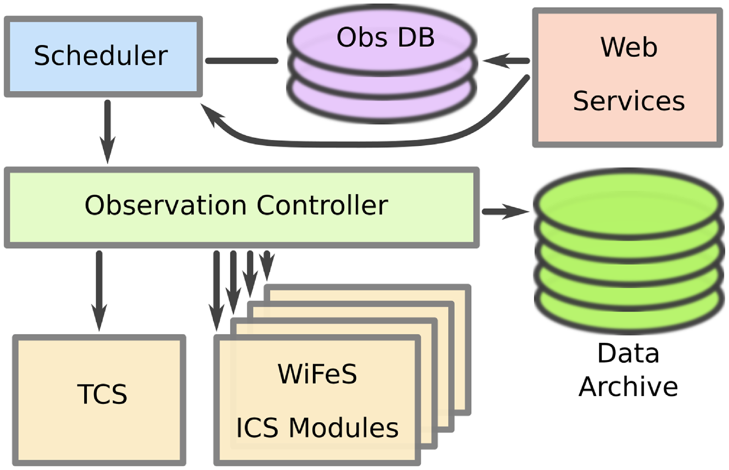
Figure 1.

Schematic of the high-level architecture of the automated observatory control system.

The Observation Controller process consumes observation blocks and coordinates all of the activities of the ICS components. Operating modes of the instrument are implemented in the business logic of this process, not in the ICS layer below. The Observation Controller is directed by the Scheduler. All decision making is implemented by the Scheduler, including assessment of the current observing conditions, observation selection, override for a ToO, or suspension of observing due to poor weather conditions. Universal coordinated time, meteorological data, and the pool of observations stored in a database underpin the operation of the Scheduler.

All processes in the system use a request-response client-server model for communication. The ICS modules report status information on request. The Observation Controller process uses a query-command-verify strategy in the implementation of all operational sequences. An initial state is never assumed and a specific final state is not required. The command-verify steps are skipped if the initial query indicates no action is necessary to progress through the sequence. Each ICS component provides a relatively thin layer of abstraction around the hardware it controls. That hardware does not need to have a native asynchronous control interface but the ICS software process must. This ensures status requests are serviced promptly, and the communication channel is not blocked. The general approach is simple and it can be formed around virtually any hardware device. It is highly suitable for retro-fitting to existing instruments with bespoke hardware and modest data rates. We used a consistent communication system for all ICS modules, but note that it was not strictly necessary to do so.

Using configurable, but pre-defined observing modes, ensures the system is operated safely and efficiently. Actions are executed in parallel where possible, and in serial when they are not. Sensibly ordering the operations to minimize overheads requires a detailed understanding of the nuances of subservient ICS components. When exploring use-cases it became clear that only a small number of very experienced 2.3 m observers had knowledge of the system sufficiently detailed to maximize time efficiency when observing. Offering only pre-defined operating modes leveraged both the practices of the most experienced observers and the detailed understanding of various subsystems held by the engineering team. It traded efficiency for flexibility, but all known modes of operation were implemented and the set of modes is readily extendable. Pre-defined operating modes also gave the development team full control of the cancellation points that are required for interrupting an observation and swiftly commencing the execution of a different sequence. Robust interruption is necessary for rapid response to ToO requests and critical for self-preservation in the event of bad weather.

2.1 Observations

Astronomers granted time on the telescope prepare their observations with a web-based tool that incorporates the Aladin Lite v2 sky viewer (Boch & Fernique Reference Boch, Fernique, Manset and Forshay2014). This facilitates construction of observation requests, comprised of observation blocks and observing constraints, and provides a mechanism for adding them into the pool of possible observations. Fig. 2 shows the tool during the preparation of a nod-and-shuffle observation for transient follow-up. The observation request includes parameters necessary for scheduling and an ordered list of observation blocks. The observation blocks are passed as - is to the Observation Controller at the point of execution, and they are opaque to the Scheduler. Observation blocks are decoded in a hierarchical process that progresses towards more specific detail about the sequence to be executed. Being opaque to all other parts of the system enabled the control system to be developed and tested with just a couple of operating modes and expanded later with development localised to the Observation Controller and the validation of submitted observations.

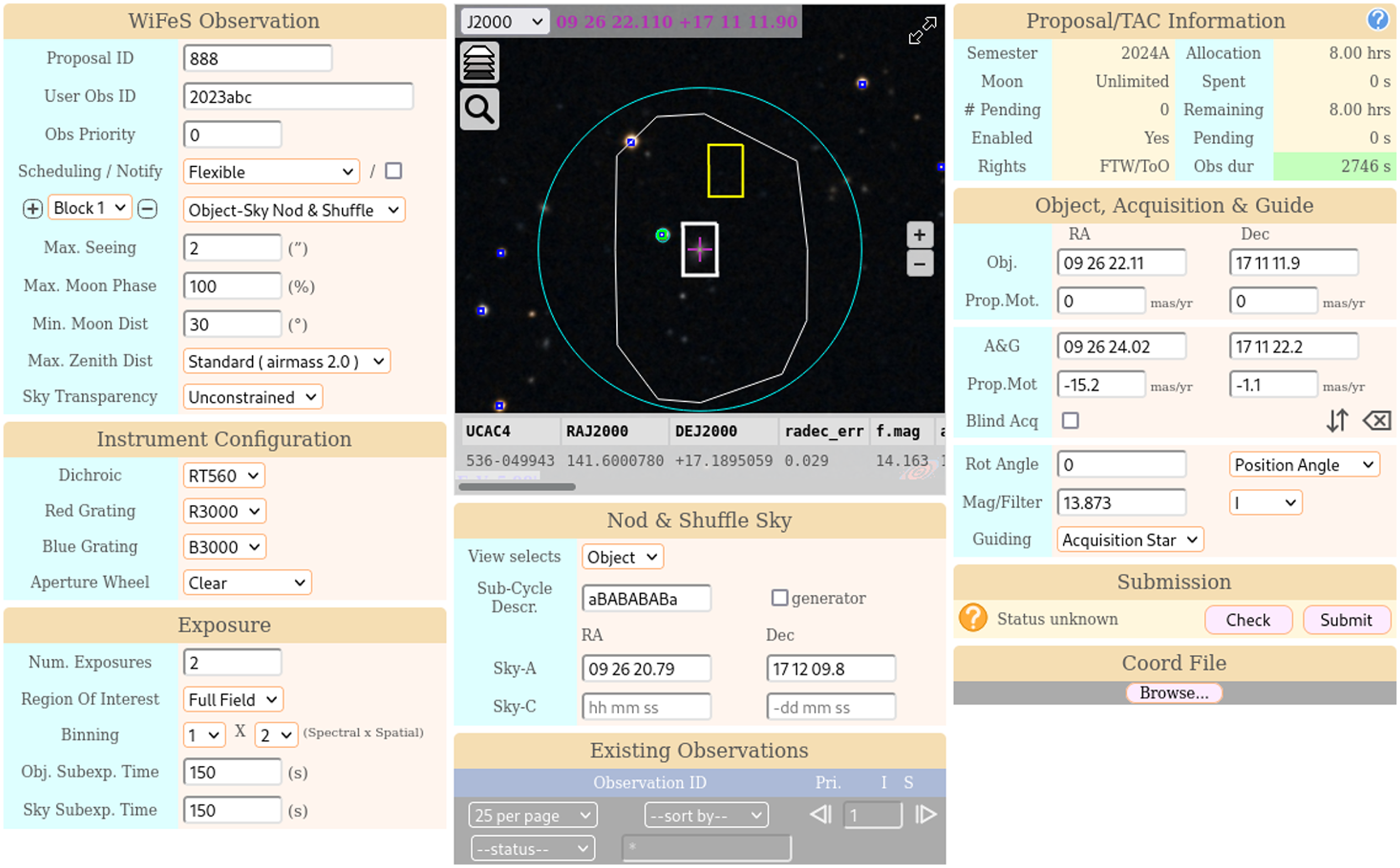
Figure 2.

A screenshot of the observation preparation tool with a complete nod-and-shuffle observation request.

2.2 Observation selection

The Scheduler partitions each 24–h period into eight sessions. The boundaries between sessions are either fixed in local-time or relative to twilight. End-user observations are allotted only to the session between astronomical twilight. The system uses some sessions for calibration observations on behalf of all users, and others are reserved for use by technical staff maintaining the facility. Observations allotted to a session are drafted into either the flexible queue or the ToO queue. The ToO queue is serviced if non-empty and an executing non-ToO observation will be terminated when a ToO observation can be serviced. Both queues are managed as priority queues using a rank metric. At the point of observation selection, the Scheduler recomputes the rank metric for each observation to take the current observing conditions, constraints, and other time dependent factors into account. The highest ranked observation is selected and execution of the list of observation blocks is delegated to the Observation Controller.

The rank metric, m, is a complex multivariate function that, broadly, implements the policies of the time allocation committee. It is structured as a weighted linear sum of functions that return values bound to the interval $[{-}1, 1]$ ,

(1) \begin{equation} m = \sum_{i} f_{i}(\bar{x})w_{i} \end{equation}

where $f_{i}$ is a policy function, $\bar{x}$ is the vector of current conditions and observation parameters, and $w_{i}$ is the weight applied to a specific policy. Each function implements one aspect of the policy, with positive values a bias towards selection and negative values biasing against selection. There are policy functions for favouring observing

• • as targets transit the meridian

• • within a specific range of seeing

• • within a specific range of lunar phase

• • at larger angular distances from the Moon

• • if the time allocation has not been consumed

• • according to scientific merit

Although each element of the policy has a role to play, the largest weights are applied to scientific merit and observing at small hour angles. To avoid having high science value observations done at large hour angles the science merit policy function has a strong negative bias at $|HA| \gt 1.5$ h. Our metric is an alternative form of the Liverpool Telescope’s original rank metric (Steele & Carter Reference Steele, Carter and Lewis1997) that does not formally separate the efficiency functions from the fairness function. The decomposition and bound range of each policy function is merely for convenience as it makes adjusting the relative weights of the policy elements reasonably intuitive.

2.3 Acquisition

The RMS pointing error of the 2.3 m is around 5 arcsec. Some science cases are tolerant of this blind pointing error owing to the $25\,\times\,38^{\prime\prime}$ field of WiFeS, but we have a goal of acquiring with an error of less than 0.5”. The field of the WiFeS acquisition and guide camera is approximately 3 arcmin across but is strongly vignetted at the edge and the center of the field. Central vignetting is due to the hole in the reflector that passes the science field to the integral field unit. A two-stage process is used to refine the pointing correction during acquisition. In the first instance the brightest point sources are extracted from the full field image (Stetson Reference Stetson1987) and compared with a source list extracted from a star catalog. The platescale and orientation of the field are accurately known, so the plate solver algorithm only searches for the translation required to best align the extracted sources with the catalog. The field is small and irregular, and the exposure depth is adaptive. It is not unusual to extract fewer than three stars. A Monte-Carlo analysis showed that pointing errors as large as 60 arcsec could be unambiguously resolved in over 99.9% of cases with only two stars detected. Fig. 3 shows the likelihood of confusion for two, three, and four star asterisms as a function of the number of stars in a 2’ field, with a 1.5” alignment tolerance. The likelihood of confusion increases with field density, but so too does the number of stars that can be extracted from the image to form the asterism. General plate solvers such as Astrometry. net (Lang et al. Reference Lang, Hogg, Mierle, Blanton and Roweis2010) use geometric hashes of three and four star asterisms and require multiple matches. Our approach is fast, does not require pre-processing of a star catalog, incorporates proper motion, and can be applied to small low density fields with irregular vignetting. It reliably resolves the issue of source ambiguity in both sparse and dense fields and largely removes blind pointing error in one iteration. The second stage is a classic iterative correction based on a subimage of the user-chosen acquisition star.

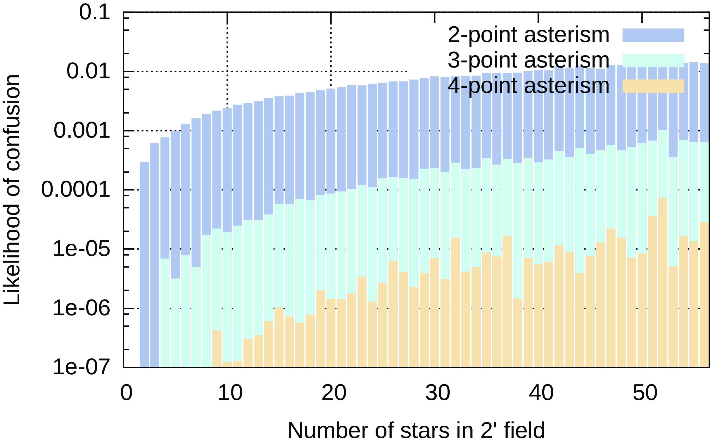
Figure 3.

The likelihood of asterism mis-identification with 2, 3, and 4 star asterisms as a function of field density in the WiFeS acquisition camera. All possible asterisms were considered from 250 000 randomly selected field centers using the UCAC4 catalog.

3. Initial six months of operation

The Automated Observatory Control System for the 2.3 m telescope and WiFeS instrument has been in continuous operation since 11th March 2023. In the six months between the vernal and autumnal equinoxes of 2023 a total of 3 377 science observations were successfully completed, with 13 of these scheduled as Target-of-Opportunity observations. The total time on target was 943 h. The efficiency of every night in this date-range in recent years was computed from the data in the archive. It is plotted against the efficiency rank in Fig. 4, where efficiency is defined as the ratio of total time observing targets to the time between astronomical twilight. Slewing between targets is not counted as observing time. Low efficiency nights are generally the result of poor weather, and an observer and the automated system both have a subjective definition of poor conditions, so variation in the tail of the distribution is expected. However at the high efficiency end of the range the nights are completely clear. This shows the automated system consistently outperforms a human observer in time-utilisation of the facility.

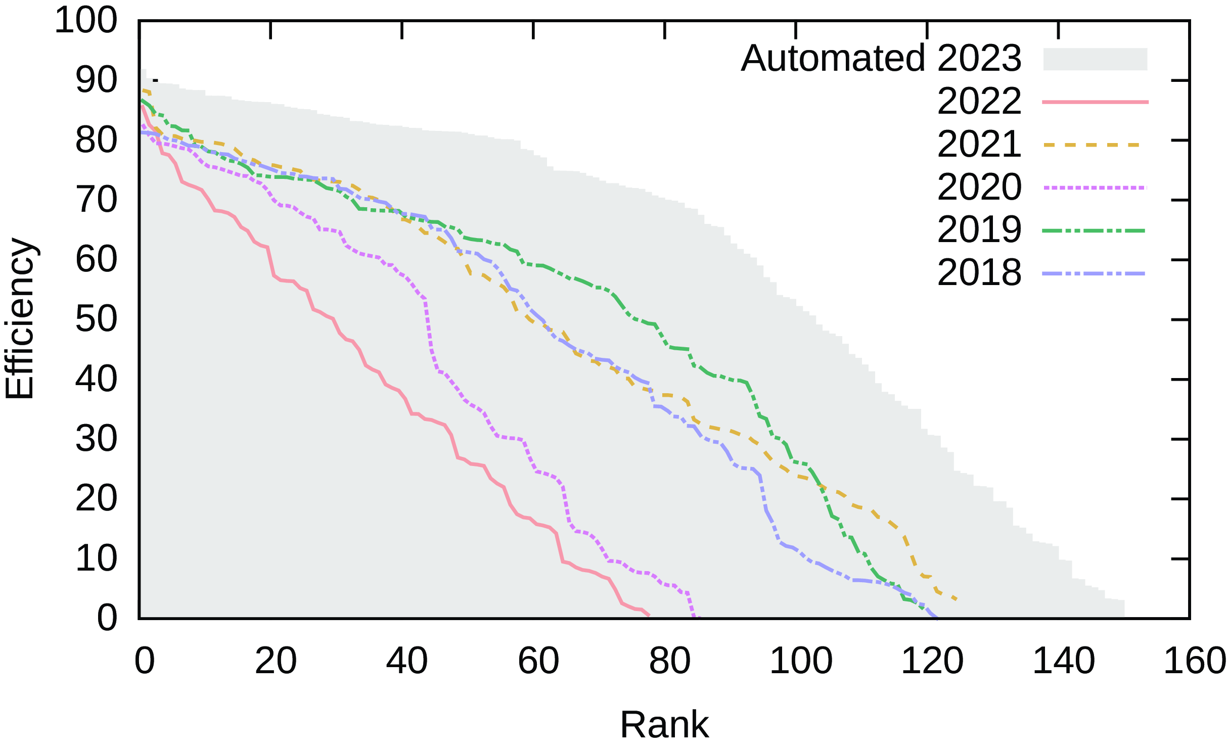
Figure 4.

Observing efficiency of each night between March 22 and September 21, ranked in order of decreasing efficiency. The automated system produced the most efficient night and consistently outperforms a human observer. The poor apparent performance in 2022 is largely due to highly under-subscribed bright time and in 2020 operation of the telescope was suspended during COVID lockdown.

The normalised distribution of time spent observing at a given hour-angle is shown in Fig. 5. This clearly shows the effect of the scheduling rank to favour observing as objects cross the meridian. The scheduling rank metric supports a reduced range of preferred hour-angle for high priority observations. This feature produces the secondary peak at $-1.5$ h, as limited competition amongst high priority observations leads to their selection as they rise. It also shows that classical scheduling leads to a broader distribution with observers marginally favouring observing to the West. The broader distribution implies observing at a higher airmass on average. This is expected given the limited time window of a classically scheduled observing run, but it is also undesirable. We have no reason to suppose the slight preference by observers for positive hour angles is either intentional or advantageous and have not sought to replicate this biased behaviour via the rank metric.

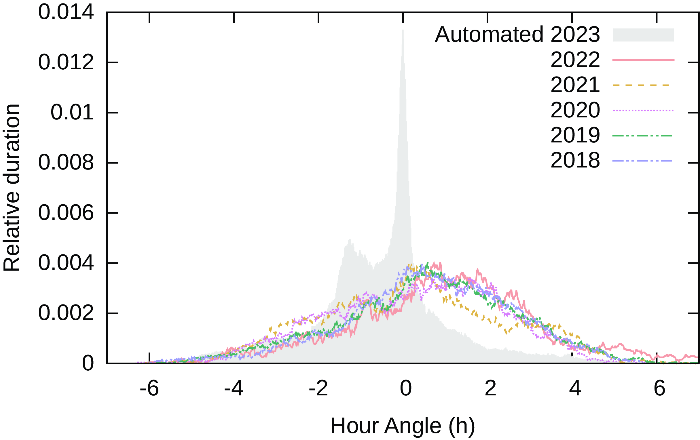
Figure 5.

Normalised distribution of time on target with hour angle. Automated scheduling results in more time spent observing near the meridian and to the East as high priority targets rise. The data from the five years prior to automated operation indicate human observers bias towards observing objects in the West.