


1. Introduction
The formation of a white layer of mist over a hot cup of coffee is a remarkable everyday example of levitation of an array of microscale droplets supported by the flow of moist air originating at the surface of evaporating liquid (Schaefer Reference Schaefer1971). The droplets form spontaneously by condensation in moist air as it is transported upwards and away from the hot liquid surface. Similar phenomena were observed for droplets over thin evaporating liquid layers on heated substrates (Fedorets Reference Fedorets2004; Fedorets, Marchuk & Kabov Reference Fedorets, Marchuk and Kabov2011; Zaitsev et al. Reference Zaitsev, Kirichenko, Ajaev and Kabov2017). For these more controlled experimental set-ups, the self-organization of droplets into large ordered arrays was discovered. Many aspects of the fascinating phenomena of levitation and self-organization of microscale droplets are described in a recent review article (Ajaev & Kabov Reference Ajaev and Kabov2021).
Despite the rapid growth of literature on experimental studies of levitating droplets, there are relatively few theoretical works on the subject. Levitation models suggest that the flow of moist air originating at the surface of an evaporating liquid can generate an upward force, estimated from the Stokes law to be large enough to balance the weight of the droplet (Fedorets et al. Reference Fedorets, Marchuk and Kabov2011; Zaitsev et al. Reference Zaitsev, Kirichenko, Kabov and Ajaev2021). However, simplifying assumptions made in the development of the models result in a number of gaps in the current understanding of levitation phenomena. Furthermore, fitting parameters are typically used to compare modelling predictions with the experimental data (Zaitsev et al. Reference Zaitsev, Kirichenko, Ajaev and Kabov2017). The key objective of the present study is to develop a comprehensive theory that does not rely on any fitting parameters and is capable of predicting both levitation height and droplet size evolution due to phase change for a wide range of conditions in which levitation is observed. Modelling of self-organization of droplets is beyond the scope of the present work, so we will focus on the configuration of an individual droplet. The theoretical tools employed in our study are based on the use of bipolar coordinates.
The mathematical foundation for the use of bipolar coordinates for Stokes flow modelling was developed in the classical study of Stimson & Jeffery (Reference Stimson and Jeffery1926). Analytical expressions for the Stokes stream function were obtained in the form of infinite series for the geometry of two solid spheres in a large volume of fluid using separation of variables in bipolar coordinates. The approach was used by Brenner (Reference Brenner1961) for geometric configurations involving isothermal spheres near flat surfaces, and generalized to situations involving heat transfer and phase change by Oguz & Sadhal (Reference Oguz and Sadhal1987), Zhang & Gogos (Reference Zhang and Gogos1991), and Oguz, Prosperetti & Antonelli (Reference Oguz, Prosperetti and Antonelli1989). In particular, the repulsion force between a hot solid surface and an evaporating spherical droplet was found as a function of the distance between the two. Recent applications of the method also include studies of variable gas density effects on drop evaporation (Cossali & Tonini Reference Cossali and Tonini2018). However, none of the previously published models is applicable directly to the configuration considered in the present study. The closest framework is the one developed by Fisher & Golovin (Reference Fisher and Golovin2007) for studies of levitation of droplets over flat liquid surfaces due to the thermocapillary effect. However, these authors did not consider phase change at the droplet surface. Furthermore, they neglected the effects of the so-called Stefan flow, a macroscopic motion of moist air that compensates for the diffusion of air molecules towards the liquid surface where evaporation takes place (Stefan Reference Stefan1873; Fuchs Reference Fuchs1959). A similar phenomenon is observed during steady-state condensation except that diffusion of air molecules is away from the surface and the flow is directed towards it.
A mathematical model of droplet levitation over an evaporating liquid layer accounting for the effects of Stefan flow was developed by Zaitsev et al. (Reference Zaitsev, Kirichenko, Ajaev and Kabov2017). It resulted in a simple analytical formula for the levitation height as a function of droplet size, but required adjustable parameters to fit the experimental data. Another limitation of this work was treating condensing droplets as point sinks. A follow-up study of Zaitsev et al. (Reference Zaitsev, Kirichenko, Kabov and Ajaev2021), while focused mostly on the experimental results, also included improvements to the model to account for the finite size of condensing droplets. A condition of uniform condensation was imposed along the droplet surface without any consideration of heat transfer in liquid or gas phases, despite the fact that strong temperature gradients have been measured in the experiments (Arinshtein & Fedorets Reference Arinshtein and Fedorets2010). As a result, neither the evaporation rate of the liquid at the layer surface nor the condensation rate at the droplet surface were determined from the model and had to be either treated as fitting parameters or evaluated based on experimental recordings of droplet size evolution. In the present study, we overcome all these limitations. A model is developed that is capable of predicting the temperature and concentration distributions, as well as flow fields, and can be used to calculate the force acting on the droplet and thus determine the conditions of levitation.
The experimental set-up of Zaitsev et al. (Reference Zaitsev, Kirichenko, Ajaev and Kabov2017, Reference Zaitsev, Kirichenko, Kabov and Ajaev2021) offers a unique opportunity to explore coupling between phase change and flow around the droplet, a topic of interest for a number of applications. For example, in spray cooling, it is important to determine the size of the droplet by the time it reaches the cooled surface (Kim Reference Kim2007). Similar issues arise in studies of droplet-laden gas flows past solid bodies (Varaksin, Vasil'ev & Vavilov Reference Varaksin, Vasil'ev and Vavilov2021). Another application is the dynamics of respiratory droplets that carry infections such as tuberculosis and COVID-19. It is well known that airborne transmission depends on the size of respiratory droplets, but the understanding of how these droplets change size due to phase change, and where they are deposited in the respiratory system under different conditions, is still incomplete; a more detailed discussion of some of these issues can be found in e.g. Kleinstreuer & Zhang (Reference Kleinstreuer and Zhang2010) and Feng et al. (Reference Feng, Kleinstreuer, Castro and Rostami2016).
2. Formulation
We consider a spherical droplet of radius  $R$ that is levitating over the surface of an evaporating liquid layer as shown in figure 1. In this set-up, motivated by the experimental studies of Zaitsev et al. (Reference Zaitsev, Kirichenko, Kabov and Ajaev2021), we start by analysing the distributions of vapour concentration $c^*$, temperature in the air around the droplet $T^*_a$, and temperature in the droplet $T^*_l.$ We non-dimensionalize these quantities using
 \begin{equation} c = \frac{c^*}{c_{sat}}, \quad T_{a,l} = \frac{T^*_{a,l}-T_s}{T_s}, \end{equation}
where  $T_s$ is the temperature at the liquid layer surface, assumed constant, and $c_{sat}$ is the equilibrium vapour saturation concentration at this temperature. Evaporation at the layer surface generates Stefan flow of moist air, of characteristic velocity $U=D M c_{sat}/(\rho R_0)$, where $D$ is the vapour diffusivity, $M$ is the molar mass of vapour, and $\rho$ is total moist air density (Sazhin Reference Sazhin2014). Since the dimensional droplet radius $R$ can change over time due to phase change, we use its characteristic value $R_0$ in the definition of $U$ and also as the scale for all length variables here. The non-dimensional governing equations then take the form
 \begin{gather} {Re}\,\frac{{\rm D} \boldsymbol{u}}{{\rm D}t} =- \boldsymbol{\nabla} p + \Delta \boldsymbol{u}, \end{gather}
 \begin{gather} \boldsymbol{\nabla} \boldsymbol{\cdot} \boldsymbol{u} = 0, \end{gather}
 \begin{gather} {Pe}_m\,\frac{{\rm D} c}{{\rm D}t} = \Delta c, \end{gather}
 \begin{gather} {Pe}\,\frac{{\rm D} T_a}{{\rm D}t} = \Delta T_a. \end{gather}
Here,  $\boldsymbol {u}$ is the moist air flow velocity scaled by $U$,
$U$,  $t$ is time scaled by $R_0/U$, and ${\rm D}/{\rm D}t$ denotes the material derivative. The effective pressure $p$ includes the contribution due to gravity and is scaled by $\mu _a U/ R_0$, where $\mu _a$ is the dynamic viscosity of air. The Reynolds number and Péclet numbers are defined by
 \begin{equation} {Re} = \frac{U \rho R_0}{\mu_a}, \quad {Pe}_m = \frac{U R_0}{D}, \quad {Pe} = \frac{U R_0}{\kappa_a}, \end{equation}
where  $\kappa _a$ is the thermal diffusivity of air. Due to liquid viscosity being much higher than $\mu _a$, the liquid phase is assumed motionless. Therefore, heat transfer in the droplet is described as pure conduction.

Figure 1. A sketch showing a spherical droplet of radius  $R$ near the surface of a heated liquid layer from which evaporation is taking place. The scaled cylindrical coordinates and levitation height are also shown.
In microscale droplet levitation experiments (Zaitsev et al. Reference Zaitsev, Kirichenko, Ajaev and Kabov2017, Reference Zaitsev, Kirichenko, Kabov and Ajaev2021), air flow velocity does not exceed  $0.1\,{\rm m}\,{\rm s}^{-1}$, so clearly the effects of air compressibility can be neglected. Droplet radius is $R_0\sim 10\,\mathrm {\mu }$m, much larger than the mean free path of the molecules in air $\lambda$, which is below 100 nm. Thus the Knudsen number $Kn = \lambda /R_0$ is assumed to be zero in the present study. For levitation experiments involving much smaller droplets, corrections that depend on the Knudsen number would have to be introduced based on the analysis of the Knudsen layers in which the gas phase is not in equilibrium. Such corrections are known to affect both the fluid flow, through the velocity slip condition, and the phase change rates (Sone Reference Sone2002; Onishi Reference Onishi1986).
Using a typical value of air flow velocity  $U=10^{-2}\,{\rm m}\,{\rm s}^{-1}$, and droplet radius $R_0=10\,\mathrm {\mu }$m, the Péclet numbers from (2.6b,c) are estimated to be $10^{-3}$ or smaller, so the governing equations for temperature and vapour concentration are reduced to Laplace's equations,
 \begin{equation} \Delta c =0, \quad \Delta T_a=0, \quad \Delta T_l=0. \end{equation}
The Reynolds number is estimated to be below  $0.01$, so the Stokes flow approximation is appropriate for moist air flow around the droplet. The modelling approach formulated here does not prevent us from describing condensing droplets as long as the condensation rate is sufficiently slow. Once the quasi-steady solutions of the governing equations are found, they can be used to determine the phase change rate and thus advance the droplet radius in time.
Our objective is to solve the equations for vapour diffusion, heat transfer and Stokes flow by separation of variables, which for the geometry of figure 1 is possible using bipolar coordinates  $\xi, \eta$ related to cylindrical coordinates via
 \begin{equation} r = \frac{\sinh \alpha \sin \eta}{\cosh \xi - \cos \eta}, \quad z = \frac{\sinh \alpha \sinh \xi}{\cosh \xi - \cos \eta}, \end{equation}
where  $\alpha \equiv \cosh ^{-1} h$, with $h$ being the levitation height scaled by $R_0$. For a better understanding of bipolar coordinates, we observe that for $\xi >0$, the curves on which the $\xi$ coordinate is constant form non-intersecting circles of increasing radius as $\xi$ decreases. In the limit of $\xi = 0$, we obtain the $r$-axis. The curves on which the $\eta$ coordinate is constant are circles that pass through two common points.
The flow in the moist air around the droplet is assumed axisymmetric and is thus described by the standard equation for the Stokes stream function,
 \begin{equation} \hat{E}^4 \psi =0, \end{equation}
where a linear operator  ${\hat E}$ is introduced such that in bipolar coordinates,
 \begin{align} \hat{E}^2 = (\cosh \xi - \mu) \left[\frac{\partial}{\partial \xi} \left( (\cosh \xi - \mu)\, \frac{\partial}{\partial \xi} \right) + (1 - \mu^2)\,\frac{\partial}{\partial \mu} \left( (\cosh \xi - \mu)\,\frac{\partial}{\partial \mu} \right) \right], \end{align}
with  $\mu =\cos \eta$. The stream function is non-dimensionalized by $R_0^2U$. Flow structure here is expected to be more complicated than in the classical studies of spherical evaporating/condensing droplets away from interfaces (Sazhin Reference Sazhin2014), but we still use the term ‘Stefan flow’ to identify clearly the physical origin of air motion.
Once the stream function is found, the scaled velocity components can be determined from
 \begin{equation} (u_{\xi} , u_{\eta}) = \frac{(\cosh \xi - \cos \eta)^2}{ \sinh^2 \alpha \sin \eta} \left( \frac{\partial \psi}{\partial \eta}, - \frac{\partial \psi}{ \partial \xi} \right). \end{equation}
 Let us now formulate the boundary conditions at the droplet surface, corresponding to  $\xi = \alpha$. The first is the fact that temperature is continuous at the liquid–air interface,
 \begin{equation} \left. T_a \right|_{\xi = \alpha} = \left. T_l \right|_{\xi = \alpha} = T_i. \end{equation}
Following previous studies (Dunn et al. Reference Dunn, Wilson, Duffy, David and Sefiane2009), we adopt a linear approximation for the dependence of the local equilibrium vapour concentration on temperature,
 \begin{equation} \left. c \right|_{\xi = \alpha}= 1 +\gamma T_i, \quad \gamma = \frac{\rho_{vT}^e}{\rho_{v}^e}\,T_s, \end{equation}
where  $\rho _{v}^e=Mc_{sat}$, and $\rho _{vT}^e$ is the rate of change of the equilibrium saturation vapour density with temperature. The condition of balance between the rate of vapour transport towards or away from the interface and the rate of phase change in our non-dimensional formulation takes the form
 \begin{equation} Q = \left. - \frac{\cosh \alpha - \cos \eta}{\sinh \alpha}\,\frac{\partial c}{ \partial \xi} \right|_{\xi=\alpha}, \end{equation}
where Q is the local condensation rate per unit interfacial area. The interfacial energy balance relates the derivatives of air and liquid temperatures in the  $\xi$ direction to the latent heat of phase change:
 \begin{equation} \left[ k\,\frac{\partial T_a}{ \partial \xi} - \frac{\partial T_l}{ \partial \xi} \right]_{\xi=\alpha} = \frac{L \sinh \alpha}{\cosh \alpha - \cos \eta}\,Q, \end{equation}
where  $k$ denotes the air-to-liquid ratio of thermal conductivities, and the non-dimensional latent heat $L$ is defined as
 \begin{equation} L = \frac{ {\mathcal{L}} D \rho_{v}^e }{k_l T_s}, \end{equation}
where  ${\mathcal {L}}$ is the dimensional latent heat, and $k_l$ is the thermal conductivity of the liquid. The parameter $L$ could be expressed in terms of Jacob number and Lewis number, but we do not use them here to keep the notation as simple as possible.
Equations (2.14) and (2.15) can be combined into
 \begin{equation} \left[ k\,\frac{\partial T_a}{ \partial \xi} - \frac{\partial T_l}{ \partial \xi} \right]_{\xi=\alpha} =-L \left. \frac{\partial c}{ \partial \xi} \right|_{\xi=\alpha}. \end{equation}
We assume  $\rho _{v}^e \ll \rho$ here, as appropriate for describing levitation at temperatures well below the boiling point, in contrast to the Leidenfrost phenomena for which (2.17) would have to be modified, as was done by e.g. Zhang & Gogos (Reference Zhang and Gogos1991). By combining the conditions of conservation of mass and energy, we effectively eliminate the phase change rate from the boundary conditions, thus time becomes a parameter in the quasi-steady model. To reflect that, we introduce a minor modification in the model by scaling all length variables by the current value of the evolving droplet radius $R$ rather than a fixed characteristic value of $R_0$. The non-dimensional droplet radius is then equal to unity.
The air flow velocity near the droplet surface has to match the Stefan flow velocity, which in our non-dimensional formulation in bipolar coordinates leads to
 \begin{equation} \left. \frac{\partial \psi}{\partial \eta} \right|_{\xi = \alpha} =-\frac{\sinh \alpha \sin \eta}{\cosh \alpha - \cos \eta} \left. \frac{\partial c}{\partial \xi} \right|_{\xi = \alpha}. \end{equation}
Motivated by large liquid-to-air viscosity ratio, we apply the no-slip condition at the droplet surface, leading to
 \begin{equation} \left. \frac{\partial \psi}{\partial \xi} \right|_{\xi = \alpha} = 0. \end{equation}
At the evaporating liquid layer surface,
 \begin{gather} \left. T_a \right|_{\xi = 0}=0, \end{gather}
 \begin{gather} \left. c \right|_{\xi = 0}=1. \end{gather}
The two conditions for the stream function at  $\xi =0$ are formulated from the same physical principles as for the droplet surface, leading to
 \begin{gather} \left. \frac{\partial \psi}{\partial \eta} \right|_{\xi = 0} =-\frac{\sinh \alpha \sin \eta}{1 - \cos \eta} \left. \frac{\partial c}{\partial \xi} \right|_{\xi = 0}, \end{gather}
 \begin{gather} \left. \frac{\partial \psi}{\partial \xi} \right|_{\xi = 0} = 0. \end{gather}
Finally, away from the droplet, the scaled temperature and concentration gradients approach the imposed values of  $G$ and $G_c$, respectively. These external gradients are established before the droplets are formed, so they can be determined from a simple geometric configuration of an evaporating liquid layer on a flat surface. The appropriate length scale for this problem is the size of the experimental set-up, so the convective heat/mass transfer is no longer negligible. However, both numerical solutions for convection near a heated horizontal surface and experimental measurements (Arinshtein & Fedorets Reference Arinshtein and Fedorets2010) suggest that in the region where droplets are levitating, typically at a distance of only ${\sim }10\,\mathrm {\mu }{\rm m}$ from the liquid layer surface, the external temperature and concentration profiles are locally well approximated by linear functions. The actual global temperature and concentration solutions will deviate from these linear profiles far away from the evaporating layer, ensuring that the concentration and temperature gradients vanish there.
3. Separation of variables
An advantage of using bipolar coordinates is that the solutions of the Laplace's equation and the Stokes stream functions can be found using the method of separation of variables (Stimson & Jeffery Reference Stimson and Jeffery1926), resulting in analytical expressions in the form of infinite series. This allows us to write the solutions for vapour density around the droplet and for the temperature distributions in the form of expansions in terms of Legendre polynomials. Specifically, the solution for scaled vapour concentration is written as
 \begin{equation} c = 1 - \frac{G_c \sinh \alpha \sinh \xi}{\cosh \xi - \cos \eta} + \sqrt{\cosh \xi - \cos \eta}\, \sum_{n=0}^{\infty} A_n \sinh \left[ \left(n+ {\frac{1}{2}}\right) \xi \right] P_n(\cos \eta), \end{equation}
where  $P_n(\cos \eta )$ are the Legendre polynomials. For the heat transfer problem, we use
 \begin{gather} T_a =- \frac{G \sinh \alpha \sinh \xi}{\cosh \xi - \cos \eta} + \sqrt{\cosh \xi - \cos \eta}\, \sum_{n=0}^{\infty} B_n \sinh \left[ \left(n+ {\frac{1}{2}}\right) \xi \right] P_n(\cos \eta), \end{gather}
 \begin{gather} T_l = \sqrt{\cosh \xi - \cos \eta}\,\sum_{n=0}^{\infty} D_n \exp\left({-\left(n+\frac{1}{2}\right) \xi}\right) P_n(\cos \eta). \end{gather}
There are no ‘cosh’ terms in the series expansions in (3.1) and (3.2) since they would not be compatible with the conditions of constant non-dimensional concentration and temperature at  $\xi =0$. The solution for the Stokes stream function is
 \begin{equation} \psi = -\frac{G_c \sinh^2 \alpha \sin^2 \eta}{2(\cosh \xi - \cos \eta)^2} + (\cosh \xi - \cos \eta)^{-3/2} \sum_{n=-1}^{\infty} W_n(\xi)\,C_{n+1}^{-1/2}(\cos \eta), \end{equation}
where  $C_{n+1}^{-1/2}$ is the Gegenbauer polynomial, and the first term corresponds to the uniform upward flow when no droplets are present. The expansion coefficients can be expressed as (Oguz et al. Reference Oguz, Prosperetti and Antonelli1989)
 $$\begin{gather} W_n(\xi) =\bar{A}_n\,\frac{\sinh n_- (\alpha - \xi)}{\sinh n_- \alpha} + \bar{B}_n\,\frac{\sinh n_- \xi}{\sinh n_- \alpha} + \bar{C}_n \left( \frac{\sinh n_- (\alpha - \xi)}{\sinh n_- \alpha} \right. \nonumber\\ -\left. \frac{\sinh n_+ (\alpha - \xi)}{\sinh n_+ \alpha} \right) + \bar{D}_n \left( \frac{\sinh n_-\xi}{\sinh n_- \alpha} - \frac{\sinh n_+ \xi}{\sinh n_+ \alpha} \right), \quad n \ge 1, \end{gather}$$
 $$\begin{gather}W_{0}(\xi) = \bar{A} \left( \cosh \frac{3 \xi}{2} + 3 \cosh \frac{\xi}{2} \right) - \bar{B} \left( \sinh \frac{3 \xi}{2} - 3 \sinh \frac{\xi}{2} \right), \end{gather}$$
 $$\begin{gather}W_{-1}(\xi) = \bar{A} \left( \cosh \frac{3 \xi}{2} + 3 \cosh \frac{\xi}{2} \right) + \bar{B} \left( \sinh \frac{3 \xi}{2} - 3 \sinh \frac{\xi}{2} \right). \end{gather}$$
 Let us now discuss the key steps in finding the solutions for concentration, temperature and flow field in the air. We start by considering the heat transfer model. The condition of continuity of temperature at the droplet surface,  $\xi = \alpha$, leads to the following relation between the coefficients $B_n$ and $D_n$:
 \begin{equation} D_n =- 2 \sqrt{2}\,\bar{n} G \sinh \alpha + {\rm e}^{\bar{n}\,\alpha} B_n \sinh \bar{n} \alpha. \end{equation}
Here, we introduced the notation  $\bar {n} \equiv n + \tfrac {1}{2}$ and used the standard expansion of the function $(\cosh \alpha - \cos \eta )^{-3/2}$ in Legendre polynomials. Equations (2.13a,b) allow us to express the coefficients of the series expansion for concentration in terms of $B_n$ as well:
 \begin{equation} A_n = \gamma B_n + R_n, \end{equation}
where
 \begin{equation} R_n = \frac{2 \sqrt{2}\,\bar{n} (G_c - \gamma G)\,{\rm e}^{-\bar{n} \alpha} \sinh \alpha }{\sinh \bar{n} \alpha }. \end{equation}
Now all coefficients of the coupled diffusion and heat transfer problems are expressed in terms of  $B_n$, so the condition (2.17) at the liquid–air interface can be used to determine their values by solving a tridiagonal linear system, as described in Appendix A.
Once the diffusion and heat transfer problems are solved, the coefficients of the fluid flow problem from (3.5)–(3.7) can be determined using the four boundary conditions for the stream function, (2.18), (2.19), (2.22) and (2.23). The procedure is straightforward, but its detailed description is presented in Appendix A since the resulting expressions are somewhat lengthy. Once the stream function is found, the dimensional upward force acting on the droplet can then be calculated using the well-known formula (Stimson & Jeffery Reference Stimson and Jeffery1926; Oguz & Sadhal Reference Oguz and Sadhal1987), expressed in our notation as
 $$\begin{align} F &= 2 \sqrt{2}\,{\rm \pi}\,\frac{\mu_{a} RU}{\sinh \alpha} \left[4\bar{A} - 4\bar{B} + \sum_{n=1}^{\infty} \left( \bar{A}_n + \frac{\bar{B}_{n} + \bar{D}_{n} - (\bar{A}_{n} + \bar{C}_{n}) \cosh n_-\alpha}{\sinh n_- \alpha} \right. \right. \nonumber\\ &\quad + \left. \left. \frac{\bar{C}_n \cosh n_+ \alpha - \bar{D}_n}{\sinh n_+ \alpha } \right) \vphantom{\sum_{n=1}^{\infty}}\right], \end{align}$$
We note that in the literature, this formula sometimes appears with the opposite sign due to a different convention in defining the Stokes stream function.
To summarize, the non-dimensional solutions for heat and mass transfer are expressed analytically as functions of  $h$,
$h$,  $k$,
$k$,  $L$,
$L$,  $\gamma$, $G$, and $G_c$, in the form of infinite series, by (3.1), (3.2), (3.3) and (3.4). The series are rapidly convergent and therefore can be truncated to a relatively small number of terms to obtain very accurate solutions; we use 20 terms in the plots shown below.
4. Results and discussion
4.1. Levitation height
The key quantity measured in the experimental studies of levitating droplets is the levitation height, so we start by discussing how this quantity can be determined from our model. Motivated by experiments of Zaitsev et al. (Reference Zaitsev, Kirichenko, Kabov and Ajaev2021), we consider a droplet of radius  $R=5\,{\rm \mu}$m at temperature $63\,^{\circ }{\rm C}$. All relevant physical properties of moist air and water at this temperature are listed in table 1. The temperature gradient in the air above the evaporating layer was not measured directly by Zaitsev et al. (Reference Zaitsev, Kirichenko, Kabov and Ajaev2021), but we estimate $G=4.625 \times 10^{-4}$ based on experimental measurements of Arinshtein & Fedorets (Reference Arinshtein and Fedorets2010) carried out under similar conditions.
Table 1. Values of physical properties of moist air and water at  $63\,^{\circ }{\rm C}$ needed to estimate the non-dimensional parameters of the model. The properties of water are from Linstrom & Mallard (Reference Linstrom and Mallard2022), the latent heat and diffusion coefficient are from engineeringtoolbox.com, and all other quantities are evaluated based on formulas from Tsilingiris (Reference Tsilingiris2008).

The condition of levitation is expressed by balancing the force  $F$ acting on the droplet from the flow, found from (3.11), and the weight of the droplet,
 \begin{equation} F = \tfrac{4}{3} {\rm \pi}R^3 \rho_l g. \end{equation}
Let us define a non-dimensional force  $\hat {F}$ according to
 \begin{equation} \hat{F} = \frac{F}{6 {\rm \pi}\mu_a R U G_c}. \end{equation}
The expression in the denominator is the Stokes force based on the dimensional flow velocity at the evaporating liquid layer surface. Assuming that the dimensional values of the temperature and concentration gradients are not affected by the presence of microscale droplets and remain constant, the quantity  $\hat {F}$ depends on the droplet radius only through the scaled levitation height $h$, therefore the levitation condition (4.1) can be written in non-dimensional form as
 \begin{equation} \hat{F}(h) = \hat{R}^2, \quad \hat{R} = R \sqrt {\frac{2 \rho_l g}{9 \mu_a U G_c}}. \end{equation}
This simple formula defines implicitly the levitation height as a function of the droplet radius and is illustrated by the plots of  $h(\hat {R})$ at different values of the scaled concentration gradient in figure 2. All curves have vertical asymptotes at finite values of $\hat {R}$, suggesting a minimum non-dimensional droplet size that can be levitated in a given concentration gradient. The minimum of $\hat {R}$ approaches a limiting value $\hat {R}^*=0.76$ when $G_c$ is increased; this critical scaled radius turns out to be the same for a range of realistic temperature gradients. Thus no levitation can be expected under any conditions when $\hat {R}<\hat {R}^*$. In dimensional terms, it means that any droplet of radius smaller than $3 \hat {R}^* \sqrt {\mu _a U G_c /(2 \rho _l g)}$ would be too light to overcome the upward force from the moist air flow. For example, if the upward flow velocity is $1\,{\rm mm}\,{\rm s}^{-1}$, then the smallest droplet size for levitation is approximately 2.2 $\mathrm {\mu }$m. Estimates based on the Stokes drag law used in all previous studies would overpredict the minimum droplet size by approximately 32 %. The discrepancy can be explained by the fact that the flow structure is different from the classical flow pattern predicted based on the no-penetration condition at the droplet surface. Specifically, pressure gradients driving liquid flow needed to maintain phase change at the droplet surface result in an additional contribution to the force not accounted for in the previous studies. This contribution is opposing the upward Stokes force and approaches a constant value when the droplet is far away from the liquid layer but still subject to the same constant temperature and concentration gradients. Thus the total force acting on the droplet from the flow has a limiting value when $h \rightarrow \infty$, explaining the vertical asymptotes in the plots of $h(\hat {R})$ in figure 2. The weight of the droplet that can balance this force defines the value of $\hat {R}^*$. Air flow patterns and their effect on the total force are explored in more detail below. We note that the minimum size requirement can also be derived for levitation of microscale droplets over solid surfaces, a configuration in which sufficiently small droplets were observed to take off rapidly while larger droplets were levitating under the same conditions (Celestini, Frisch & Pomeau Reference Celestini, Frisch and Pomeau2012).

Figure 2. Levitation height as a function of droplet radius in non-dimensional coordinates for  $k=0.0413$, $\gamma =14.3$, $L=0.0514$, $G=4.625 \times 10^{-4}$, and different values of $G_c$.
Another characteristic feature of the curves seen in figure 2 is that they decay rapidly as  $\hat {R}$ is increased, suggesting that the thickness of the gap between the droplet and the evaporating layer decreases quickly when the droplets become larger. While formally the thickness becomes zero only in the limit as $\hat {R} \rightarrow \infty$, experimental observations show clearly that droplets often merge with the liquid layer when the scaled levitation height is near 1.1 as a result of random fluctuations of the droplet position or wavy deformations of the layer surface (Ajaev & Kabov Reference Ajaev and Kabov2021). For realistic values of the temperature and concentration gradients, $h$ is always below 1.1 when $\hat {R}$ is near 3 or above. Thus we can summarize the discussion here by stating that levitation can be expected only in a relatively narrow range of $\hat {R}$ between 0.76 and $\sim$3, a conclusion that provides useful guidance for future experimental studies.
4.2. Comparison with experiments
Zaitsev et al. (Reference Zaitsev, Kirichenko, Kabov and Ajaev2021) report careful measurements of the droplet levitation height for a range of droplet sizes and different temperatures. While not measured experimentally, the scaled concentration gradient  $G_c$ can be estimated from the videos of droplets travelling downwards before they join the array, as seen e.g. in figure 4 of Kabov et al. (Reference Kabov, Zaitsev, Kirichenko and Ajaev2017). When the downward speed $U_{0}$ is approximately constant, the forces acting on the droplet balance, leading to the equation
 \begin{equation} F + 6 {\rm \pi}\mu_a U_0 R = \tfrac{4}{3} {\rm \pi}R^3 \rho_l g, \end{equation}
where  $F$ refers to the limiting value of the force calculated according to (3.11) at $h \rightarrow \infty$; we choose $h=50$ based on the shape of the $F(h)$ curve, and use $R\approx 4.4\,\mathrm {\mu }{\rm m}$ (the downward moving droplets seen in the videos are slightly smaller than the ones levitating in the array). The resulting estimate to be used in the levitation condition is $G_c=\hat {G}_c R$ with $\hat {G}_c=287\ {\rm m}^{-1}$. Since the dimensional concentration profile is independent of the droplet radius, it is convenient to define $\hat {G}_c = G_c/R$, a quantity that also does not vary with droplet size. For the reference case discussed in the previous subsection, that corresponds to $G_c=1.435 \times 10^{-3}$. Using the same general procedure as for figure 2 with the value of $G_c$ matching the experiment, the blue theoretical curve in figure 3 is obtained. Next, the raw data on levitation height versus droplet radius from Zaitsev et al. (Reference Zaitsev, Kirichenko, Kabov and Ajaev2021) is converted into our non-dimensional variables and shown by filled squares in the same figure. Given that no fitting parameters were used in our derivation of levitation conditions, the agreement is very good, especially since many simplifying assumptions were made in the model. In particular, we neglected convective effects that could reduce the spatial non-uniformity of the phase change rate and thus decrease the contribution to the force due to phase change at the droplet surface, discussed in more detail in the next subsection. Thus the net upward force acting on the droplet from the flow is increased, and the droplet can levitate at a larger height. This is consistent with the slight underprediction of the levitation height seen in figure 3, although it is difficult to make definitive conclusions due to significant scatter in the experimental data, caused most likely by the limitation of the optical resolution of droplet images.

Figure 3. Comparison of the predicted levitation height with experimental data at  $63\,^{\circ }{\rm C}$ from Zaitsev et al. (Reference Zaitsev, Kirichenko, Kabov and Ajaev2021). The blue curve is predicted by the theory, with $\hat {G}_c=287\ {\rm m}^{-1}$ and the same values of other non-dimensional parameters as in the previous figure. Filled squares represent experimental measurements based on optical recordings of size and location of levitating droplets, expressed in our non-dimensional variables.
While experimental studies have been conducted for a range of substrate temperatures, our model is limited by the condition of the equilibrium vapour density being much smaller than the total moist air density, needed to justify (2.17). Therefore, for comparison we used the lowest temperature at which experiments were conducted. We expect that using the more accurate nonlinear version of (2.17) – as discussed in the context of the Leidenfrost phenomenon by e.g. Zhang & Gogos (Reference Zhang and Gogos1991) – would improve the comparisons such as that in figure 3 and also allow us to justify comparisons at higher temperatures. However, using such more accurate conditions would not allow one to obtain analytical solutions, the key benefit of the proposed approach, so we do not pursue this here. The issue will be addressed in future numerical studies.
4.3. Heat transfer and phase change rates
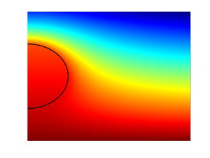
The upward force  $F$ acting on the droplet depends on the phase change rates at the droplet surface, so physical understanding of levitation requires a more detailed discussion of the solution of the heat transfer problem, the subject of the present subsection. For a better illustration of the small spatial temperature variations inside and around the droplet, we redefine the scaled temperature here according to
 \begin{equation} \hat{T}= \frac{T^*-T^*_{min}}{T^*_s-T^*_{min}}, \end{equation}
where  $T^*_{min}$ is the minimum value of the temperature in the domain shown. In the limit of negligible phase change at the interface ( $L=0$ in our formulation), illustrated in figure 4(a), the solution found by Fisher & Golovin (Reference Fisher and Golovin2007) is recovered. A key feature of their solution is the nearly uniform temperature distribution within the droplet, with the temperature gradients there being much lower than the imposed temperature gradient in the surrounding air. These observations can be explained by the fact that liquid is much more thermally conductive than air, so even small changes in the temperature inside the droplet are sufficient to balance the changes in heat flux from the air side of the interface. However, incorporating the phase change into the model leads to qualitatively different temperature distributions. As the value of $L$ is increased, corresponding to a larger contribution of latent heat in the overall energy balance, temperature gradients develop, supporting the phase change. This is seen clearly in figure 4(b), corresponding to realistic values of the parameters $L$ and $\gamma$. The average droplet temperature is significantly higher than in figure 4(a), so stronger temperature gradients near the interface can be established, as needed to balance the latent heat release due to condensation at the droplet surface. The fact that the droplet mass is increasing under the conditions corresponding to figure 4(b) is well established by experimental observations (Zaitsev et al. Reference Zaitsev, Kirichenko, Ajaev and Kabov2017, Reference Zaitsev, Kirichenko, Kabov and Ajaev2021) and is also predicted by our model, as discussed in more detail in the next paragraph.

Figure 4. Solutions for the temperature in both moist air and liquid for (a) the model that neglects phase change at the droplet surface, and (b) the model with  $L=0.0514$, $\gamma =14.3$, based on levitation experiments with microscale water droplets (Zaitsev et al. Reference Zaitsev, Kirichenko, Kabov and Ajaev2021). For both cases, $k=0.0413$ and $\hat {G}_c=287\ {\rm m}^{-1}$.
Once the coefficients  $B_n$ are determined, (3.9) together with (3.1) can be used to obtain the vapour concentration distributions and the interfacial scaled condensation mass flux $J_c \equiv G_c^{-1}\,\partial c/ \partial n$, which is the key measure of the phase change rate at the interface, with negative values corresponding to evaporation. The definition here is based on the fact that the natural scale for all concentration gradients is set by the value at the surface of the evaporating layer. We also define the angle $\theta$, measured from the direction of the $z$-axis, as is normally done in the definition of spherical coordinates. The condensation flux profiles $J_c(\theta )$ then provide complete information on the phase change rate as the system is assumed axisymmetric. For droplets far away from the liquid layer, the shapes of the flux profiles are similar but the average flux value is reduced gradually as the droplet approaches the liquid layer. Examples of such profiles are the blue and green lines in figure 5. Note that for each profile, the local condensation rate is highest at the bottom of the droplet, $\theta ={\rm \pi}$. This conclusion is rather unexpected since hotter regions are often associated with reduced condensation or increased evaporation in heat transfer systems, and the bottom part of the droplet surface is at a higher temperature, due to proximity to the heater, than the top part. To resolve the apparent contradiction, we recall that the droplets are in strong concentration gradient and therefore the air around the droplet near the top has significantly lower vapour concentration.

Figure 5. Condensation flux as a function of the scaled vertical coordinate for  $L=0.0514$, $\gamma =14.3$, $k=0.0413$, $\hat {G}_c=287\ {\rm m}^{-1}$, and different droplet locations. The bottom of the droplet corresponds to $\theta ={\rm \pi}$.
The red line in figure 5, corresponding to the lowest levitation height, shows that the condensation rate at the bottom does not decrease as much as one might expect from comparing the blue and green curves. We believe this to be the effect of geometric confinement. The vapour originating from the surface of the liquid layer is not evacuated efficiently enough due to the limitations of viscous flow in the gap between the droplet and the liquid layer, leading to an increase in vapour partial pressure and thus promoting condensation. The limited ability of flow to remove vapour from narrow air gaps is well established in the studies of levitating droplets over liquid pools by e.g. Maquet et al. (Reference Maquet, Sobac, Darbois-Texier, Duchesne, Brandenbourger, Rednikov, Colinet and Dorbolo2016) and van Limbeek et al. (Reference van Limbeek, Sobac, Rednikov, Colinet and Snoeijer2019). Another interesting observation from figure 5 is that for sufficiently small levitation heights, there is actually evaporation rather than condensation in the part of the droplet surface near the top ( $\theta =0$), an indication of vapour concentration in surrounding air being low enough to result in the reversal of the direction of phase change.
Let us now discuss how phase change affects the total force acting on the droplet. Condensation implies that there is flow towards the droplet surface, and to maintain that viscous flow, a pressure gradient is needed, with lower pressure near the surface. This pressure reduction is most significant where the condensation is the strongest, i.e. near the bottom of the droplet. Thus the additional component of force due to non-uniform phase change, identified previously, is pushing the droplet downwards. This is the opposite to the situation encountered in the Leidenfrost effect where evaporation leads to increased pressure. The simplified explanation here does not describe accurately the pressure field and the role of shear stresses in the force balance, but we still feel it provides a useful insight into the results found from the complete model above, which does not have these limitations.
We note that the phase change rate depends not only on the vapour concentration around the droplet but also on the equilibrium saturation value, which in turn is a function of temperature. Thus using the physically realistic value of  $\gamma$ is essential for estimating correctly the condensation fluxes here. In fact, we observed that neglecting the dependence of equilibrium concentration on temperature by choosing $\gamma =0$ would lead to predictions of much stronger evaporation from the droplet surface, in direct contradiction to experimental data showing that droplet radius is gradually increasing rather than decreasing (Zaitsev et al. Reference Zaitsev, Kirichenko, Ajaev and Kabov2017, Reference Zaitsev, Kirichenko, Kabov and Ajaev2021; Fedorets et al. Reference Fedorets, Marchuk and Kabov2011). Thus models using a constant value of equilibrium concentration independent of temperature cannot capture accurately droplet dynamics in the presence of phase change, a conclusion consistent with many previous studies, most notably those of evaporating sessile droplets on heated substrates (Dunn et al. Reference Dunn, Wilson, Duffy, David and Sefiane2009).
The predictions of local phase change rates, such as the ones illustrated in figure 5, are obtained for a fixed value of the droplet radius, a quantity that is expected to change as a result of condensation. While our model does not account for unsteady effects in heat and mass transport, as discussed in § 2, it can still be used to describe radius evolution in a quasi-steady fashion, i.e. by estimating the condensation rate from the steady problem and then using it to advance the droplet surface.
Classical quasi-steady models of evaporating and condensing droplets away from interfaces predict the square of a spherical droplet diameter to be a linear function of time (Sazhin Reference Sazhin2014; Sirignano Reference Sirignano2014). This so-called  $D^2$ law is supported by numerous experimental studies, but there are also well-documented deviations from it when the droplets are near heated solid or liquid surfaces, and when the phase change effects are significant (Quéré Reference Quéré2013; Maquet et al. Reference Maquet, Sobac, Darbois-Texier, Duchesne, Brandenbourger, Rednikov, Colinet and Dorbolo2016; Ajaev & Kabov Reference Ajaev and Kabov2021). In particular, Maquet et al. (Reference Maquet, Sobac, Darbois-Texier, Duchesne, Brandenbourger, Rednikov, Colinet and Dorbolo2016) observed a linear decrease of the radius of an evaporating droplet floating on a gas cushion above a liquid surface, and provided a theoretical explanation for this dependence. They considered evaporating rather than condensing droplets, while the liquid below the droplet was non-volatile. For the slowly condensing droplets of interest to the present study, several previous models treated condensation rate as a fitting parameter (Zaitsev et al. Reference Zaitsev, Kirichenko, Ajaev and Kabov2017, Reference Zaitsev, Kirichenko, Kabov and Ajaev2021), while experimental measurements conducted under different conditions indicate that both the $D^2$ law (Fedorets, Marchuk & Kabov Reference Fedorets, Marchuk and Kabov2013) and a linear increase of the radius (Shatekova Reference Shatekova2020) are possible. Let us now discuss what our model predicts.
Based on the condition of conservation of mass, the rate of change of droplet mass has to match the total flux of vapour transported towards/away from the interface. To formulate this condition in non-dimensional form, it is convenient to interpret the characteristic value of the radius  $R_0$ as the value at $t=0$, i.e. when the recording of the radius evolution starts, and introduce new non-dimensional length and time variables
 \begin{equation} \tilde{R}=\frac{R}{R_0}, \quad \tilde{t} = \frac{D \rho_v^e \hat{G}_c t}{2 \rho_l R_0}. \end{equation}
The mass balance condition can then be expressed in non-dimensional form as
 \begin{equation} \frac{{\rm d} \tilde{R}}{{\rm d} \tilde{t}} = \int_o^{\rm \pi} J_c(\theta) \sin \theta \,{\rm d}\theta, \end{equation}
with  $J_c(\theta )$ being the condensation flux profile discussed above and shown in figure 5. Equation (4.7) is a first-order ordinary differential equation that was solved using a standard Matlab solver, with the height $h$ adjusted at each time step to reflect the actual location of the levitating droplet; the resulting evolution of the non-dimensional radius is shown by the solid line in figure 6. The dashed line shows the prediction of the classical $D^2$ law, which clearly suggests slower condensation. Most importantly, the blue line is close to linear dependence, in qualitative agreement with the data from a recent experimental study of Shatekova (Reference Shatekova2020). The actual value of the rate of change of radius in experiments, $1.7 \times 10^{-7}\,{\rm m}\,{\rm s}^{-1}$, is lower than predicted by our model. We believe that the discrepancy could be due to convective effects neglected in our model.

Figure 6. Droplet radius as a function of time as predicted by our model (solid line) and by the classical  $D^2$ law (dashed line).
4.4. Flow patterns
Previous studies of levitating droplets assumed a simple pattern of streamlines flowing around the droplet, as sketched e.g. in Fedorets et al. (Reference Fedorets, Marchuk and Kabov2013), leading to the force estimate via the Stokes drag law. However, our calculation of force in § 4.1 clearly shows that to be inaccurate, and thus suggests that the flow pattern should be different. With all coefficients of the expansion of  $\psi$ now being determined, we are in position to study the air flow patterns around the droplet. Typical results are illustrated in figure 7 for two different scaled levitation heights. The flow patterns are indeed different from the simple case of viscous flow around a sphere. Under the droplet, the streamline density is reduced, suggesting reduction in the speed of flow originating at the layer surface as compared to the regions away from the droplet. The streamlines suggest that liquid evaporated from the flat layer condenses at the droplet surface. This condensation is likely the limiting mechanism leading to reduction of evaporation rate and thus flow velocity. There are streamlines originating at the top of the droplet, corresponding to the evaporation region identified in the previous subsection. The extent of the evaporation region increases with the reduction of the scaled levitation height. The streamlines originating far from the droplet follow the same general patters as for classical viscous flow around a sphere.

Figure 7. Pattern of streamlines around the levitating droplet based on the solution for the Stokes stream function at different scaled levitation heights: (a)  $h=2$, and (b) $h=1.5$.
5. Conclusions
We develop a comprehensive theoretical model of droplet levitation over surfaces of evaporating liquids by solving coupled vapour diffusion and two-phase heat transfer problems, followed by determination of the flow field around the droplet and calculation of the force acting on it. The method of separation of variables in bipolar coordinates is used to obtain analytical solutions in the form of infinite but rapidly converging series expansions. In contrast to all previous models of levitation phenomena, no fitting parameters are used to determine levitation height as a function of droplet radius.
While the general mechanism of levitation due to the balance of gravity and viscous force from the upward air flow was elucidated by Fedorets et al. (Reference Fedorets, Marchuk and Kabov2011), their qualitative study does not explain why all droplets are levitating at the same height. One possible explanation is that changes in the local evaporation rate at the flat layer surface as the droplet approaches it result in changes in the upward force. This scenario was considered under the assumption of uniform condensation rate at the droplet surface by Zaitsev et al. (Reference Zaitsev, Kirichenko, Kabov and Ajaev2021). However, this approach misses another contribution to the force, which is due to the changes in flow structure around the droplet caused by non-uniform phase change at its surface. We found that the second contribution is also important. Accounting for both allowed us to obtain the levitation conditions that are in good agreement with the experimental data. We found that levitation is possible only when the non-dimensional radius defined according to (4.3a,b) is in the range between 0.76 and  $\sim$3. The previously neglected contribution to force due to a non-uniform phase change rate can also be important in situations not related to levitation, e.g. for microscale droplets travelling through regions of temperature and concentration gradients. An example of such a situation is a respiratory droplet exhaled or inhaled during the normal breathing cycle: the temperature and humidity in the respiratory airways can be dramatically different from those of the external air.
Detailed analysis of the heat transfer model indicates significantly higher average droplet temperatures compared to predictions of models neglecting phase change at the droplet surface. In contrast to many other applications, the hottest bottom part of the droplet surface facing the evaporating layer is where most condensation takes place. This unexpected result is explained by the concentration of vapour there being higher than near the top. The solution for heat transfer is used to estimate the rate of change of droplet radius. Deviations from the classical  $D^2$ law are found, in qualitative agreement with experimental results showing nearly linear growth of the radius. The slight overprediction of the rate of growth of the radius by our theory can be attributed to the neglect of convective effects.
Levitating droplets observed in experiments span a range of sizes from a few microns to  $\sim$0.1 mm. While the applicability of the model to the larger droplets is limited mostly by our assumption of small Péclet numbers, the smaller droplets may also be influenced by physical effects which we neglected here, such as thermophoresis, diffusiophoresis, and the presence of Knudsen layers near interfaces. Studies of all these, as well as detailed numerical simulations of convective flows inside and around the droplet, provide possible new directions for future investigations.
The thermocapillary effect (Young, Goldstein & Block Reference Young, Goldstein and Block1959) could contribute to levitation conditions for both smaller and larger droplets. However, a study of microscopic droplets near a dry solid surface under similar temperature gradients by Ajaev, Zaitsev & Kabov (Reference Ajaev, Zaitsev and Kabov2021) suggested that its contribution is secondary to that of phase change, so we do not include it here. Note that according to figure 4, the degree of temperature variation along the droplet surface is much smaller than may be expected based on the external temperature gradient. Still, a more detailed investigation of the thermocapillary effect in the context of levitating droplets is certainly of interest.
Acknowledgments
The authors are grateful to D.P. Kirichenko for useful discussions and providing the raw experimental data.
Funding
The work was supported by the US National Science Foundation under grant no. DMS-2009741.
Declaration of interests
The authors report no conflict of interest.
Appendix A
The tridiagonal system of equations for the vector of coefficients  $B_n$ for the model of heat transfer and diffusion in § 3 is defined by
 \begin{align} &
{-\tfrac{1}{2}} n \left( (k + L \gamma) \cosh n_-
\alpha + \sinh n_- \alpha \right) B_{n-1} + \left[ (k + L
\gamma) \left({\tfrac{1}{2}} \cosh n_+ \alpha
\right. \right. \nonumber\\ &\quad + \left.\left. n
\cosh \bar{n} \alpha \cosh \alpha \right) - \sinh \bar{n}
\alpha\, \left({\tfrac{1}{2}} \sinh \alpha -
\bar{n} \cosh \alpha\right) \right] B_n - {
\tfrac{1}{2}} (n+1) \left( (k + L \gamma) \cosh n_+ \alpha
\right. \nonumber\\ &\quad + \left. \sinh n_+ \alpha
\right) B_{n+1} = 2 \sqrt{2}\,\bar{n} G \sinh
\alpha \left(\bar{n} \cosh \alpha -
{\tfrac{1}{2}} \sinh \alpha \right) {\rm
e}^{-\bar{n} \alpha} \nonumber\\ &\quad - \left( n \cosh
\alpha \cosh \bar{n} \alpha + {\tfrac{1}{2}} \cosh n_+
\alpha\right) L R_n + {\tfrac{1}{2}} n L R_{n-1} \cosh n_-
\alpha \nonumber\\ &\quad + {\tfrac{1}{2}} (n+1) L R_{n+1}
\cosh n_+ \alpha - \sqrt{2}\,G \sinh \alpha ( n n_-\,
{\rm e}^{-n_- \alpha} + (n+1) n_+\,{\rm e}^{-n_+
\alpha} ) \nonumber\\ &\quad +
\sqrt{2}\,{\rm e}^{-\bar{n} \alpha} \sinh \alpha
(kG+LG_c)\left( \cosh \alpha - 2 \bar{n} \sinh \alpha
\right),
\end{align}
\begin{align} &
{-\tfrac{1}{2}} n \left( (k + L \gamma) \cosh n_-
\alpha + \sinh n_- \alpha \right) B_{n-1} + \left[ (k + L
\gamma) \left({\tfrac{1}{2}} \cosh n_+ \alpha
\right. \right. \nonumber\\ &\quad + \left.\left. n
\cosh \bar{n} \alpha \cosh \alpha \right) - \sinh \bar{n}
\alpha\, \left({\tfrac{1}{2}} \sinh \alpha -
\bar{n} \cosh \alpha\right) \right] B_n - {
\tfrac{1}{2}} (n+1) \left( (k + L \gamma) \cosh n_+ \alpha
\right. \nonumber\\ &\quad + \left. \sinh n_+ \alpha
\right) B_{n+1} = 2 \sqrt{2}\,\bar{n} G \sinh
\alpha \left(\bar{n} \cosh \alpha -
{\tfrac{1}{2}} \sinh \alpha \right) {\rm
e}^{-\bar{n} \alpha} \nonumber\\ &\quad - \left( n \cosh
\alpha \cosh \bar{n} \alpha + {\tfrac{1}{2}} \cosh n_+
\alpha\right) L R_n + {\tfrac{1}{2}} n L R_{n-1} \cosh n_-
\alpha \nonumber\\ &\quad + {\tfrac{1}{2}} (n+1) L R_{n+1}
\cosh n_+ \alpha - \sqrt{2}\,G \sinh \alpha ( n n_-\,
{\rm e}^{-n_- \alpha} + (n+1) n_+\,{\rm e}^{-n_+
\alpha} ) \nonumber\\ &\quad +
\sqrt{2}\,{\rm e}^{-\bar{n} \alpha} \sinh \alpha
(kG+LG_c)\left( \cosh \alpha - 2 \bar{n} \sinh \alpha
\right),
\end{align}
with the quantity  $R_n$ defined by (3.10). The solution of this linear system is obtained using Matlab and then used to determine the coefficients $D_n$ of the temperature series in the liquid phase, as well as vapour concentration solution.
Let us now turn to the coefficients of the solution for the stream function from (3.5)–(3.7). Note that while the flow solution is given in terms of Gegenbauer polynomials, it can be converted to a series in Legendre polynomials using the identity
 \begin{equation} C_{n+1}^{-1/2}(\mu)= \frac{1}{2n+1} \left(P_{n-1}(\mu) - P_{n+1}(\mu) \right). \end{equation}
The application of this formula together with  $W_n(0)=\bar {A}_n$ and the key properties of Legendre polynomials to the condition (2.22) at the droplet surface leads to equations for the coefficients $\bar {A}_n$:
 $$\begin{align} &\frac{2n-3}{4
n_-}\,\bar{A}_{n-1} - \bar{A}_n + \frac{2n+5}{4
n_+}\,\bar{A}_{n+1} = \sinh \alpha \left[
\frac{n(n-1)}{4n_-}\,A_{n-2} - n A_{n-1} \right.
\nonumber\\ &\quad +\left. \left( \bar{n} + \frac{(n+1)^2}{4 n_+}
+ \frac{n^2}{4 n_-} \right) A_n - (n+1) A_{n+1} +
\frac{(n+1)(n+2)}{4 n_+}\,A_{n+2} \right],
\end{align}$$
$$\begin{align} &\frac{2n-3}{4
n_-}\,\bar{A}_{n-1} - \bar{A}_n + \frac{2n+5}{4
n_+}\,\bar{A}_{n+1} = \sinh \alpha \left[
\frac{n(n-1)}{4n_-}\,A_{n-2} - n A_{n-1} \right.
\nonumber\\ &\quad +\left. \left( \bar{n} + \frac{(n+1)^2}{4 n_+}
+ \frac{n^2}{4 n_-} \right) A_n - (n+1) A_{n+1} +
\frac{(n+1)(n+2)}{4 n_+}\,A_{n+2} \right],
\end{align}$$
valid for  $n > 1$. Two additional equations, corresponding to $n=0$ and $n=1$, can be written in the same form by replacing $\bar {A}_{-1}$ and $\bar {A}_{0}$ with $4 \bar {A}$ while also setting $A_n$ to zero for $n<0$. The resulting tridiagonal linear system of equations for $\bar {A}_n$ has been solved using Matlab. Similarly, observing that $W_n(\alpha )=\bar {B}_n$ together with (2.18) leads to the formula
 $$\begin{align} &\frac{2n-3}{4
n_-}\,\bar{B}_{n-1} -\cosh \alpha \bar{B}_n + \frac{2n+5}{4
n_+}\,\bar{B}_{n+1} \nonumber\\ &\quad = \sinh \alpha \left[ \cosh
\alpha\left(\bar{n} \cosh \alpha \cosh \bar{n}
\alpha +\tfrac{1}{2} \sinh \alpha
\sinh \bar{n} \alpha \right) A_n - S^{(1)}_n +
S^{(2)}_n \right],
\end{align}$$
$$\begin{align} &\frac{2n-3}{4
n_-}\,\bar{B}_{n-1} -\cosh \alpha \bar{B}_n + \frac{2n+5}{4
n_+}\,\bar{B}_{n+1} \nonumber\\ &\quad = \sinh \alpha \left[ \cosh
\alpha\left(\bar{n} \cosh \alpha \cosh \bar{n}
\alpha +\tfrac{1}{2} \sinh \alpha
\sinh \bar{n} \alpha \right) A_n - S^{(1)}_n +
S^{(2)}_n \right],
\end{align}$$where
 \begin{align} S^{(1)}_n &= \left(2 n_- \cosh \alpha \cosh n_- \alpha +\frac{1}{2} \sinh \alpha \sinh n_- \alpha \right) \frac{n A_{n-1}}{2 n_-} \nonumber\\ &\quad + \left(2 n_+ \cosh \alpha \cosh n_+ \alpha +\frac{1}{2} \sinh \alpha \sinh n_+ \alpha \right) \frac{(n+1) A_{n+1}}{2 n_+}, \end{align}
 \begin{align} S^{(2)}_n &= \cosh\left[\left(n-\frac{3}{2}\right) \alpha \right] \frac{n(n-1)}{4n_-}\,A_{n-2} + \left( \frac{(n+1)^2}{4 n_+} +\frac{n^2}{4 n_-} \right) A_n \cosh \bar{n} \alpha \nonumber\\ &\quad +\cosh\left[ \left(n+\frac{5}{2}\right) \alpha \right] \frac{(n+1)(n+2)}{4n_+}\,A_{n+2}, \end{align}
all applied at  $n > 1$, with $n=0$ and $n=1$ treated as special cases, similarly to the calculation of $\bar {A}_n$ above. Once the coefficients $\bar {A}_n$ and $\bar {B}_n$ are determined, (2.23) can be used to express $\bar {D}_n$ in terms of the other coefficients:
 \begin{equation} \bar{D}_n = \frac{n_- \bar{A}_n \coth n_- \alpha - n_- \bar{B}_n\,\text{csch} \, n_- \alpha + \bar{C}_n (n_- \coth n_- \alpha - n_+ \coth n_+ \alpha)}{ n_-\,\text{csch} \, n_- \alpha - n_+\, \text{csch} \, n_+ \alpha}. \end{equation}
Finally, (2.19) leads to
 $$\begin{align}
&-\frac{n+1}{2n_-}\,W'_{n-1}(\alpha) +\cosh
\alpha\,W'_n(\alpha) - \frac{n}{2 n_+}\,W'_{n+1}(\alpha) =
\frac{3}{2} \sinh \alpha \bar{B}_n \nonumber\\ &\quad\qquad\ \ -
\frac{G_c \sinh^2 \alpha}{2 \sqrt{2}} \left[ \left(
\frac{n(n+2)}{n_+} + \frac{n^2-1}{2n_-} - 4 \bar{n}\right)
{\rm e}^{-\bar{n} \alpha} \right. \notag\\
&\quad\qquad\ \ + \left. \frac{n(n+1)}{n_-}\,{\rm e}^{-(n-3/2) \alpha}
+\frac{n(n+1)}{n_+}\,{\rm e}^{-(n+5/2) \alpha}
\right],
\end{align}$$
$$\begin{align}
&-\frac{n+1}{2n_-}\,W'_{n-1}(\alpha) +\cosh
\alpha\,W'_n(\alpha) - \frac{n}{2 n_+}\,W'_{n+1}(\alpha) =
\frac{3}{2} \sinh \alpha \bar{B}_n \nonumber\\ &\quad\qquad\ \ -
\frac{G_c \sinh^2 \alpha}{2 \sqrt{2}} \left[ \left(
\frac{n(n+2)}{n_+} + \frac{n^2-1}{2n_-} - 4 \bar{n}\right)
{\rm e}^{-\bar{n} \alpha} \right. \notag\\
&\quad\qquad\ \ + \left. \frac{n(n+1)}{n_-}\,{\rm e}^{-(n-3/2) \alpha}
+\frac{n(n+1)}{n_+}\,{\rm e}^{-(n+5/2) \alpha}
\right],
\end{align}$$
which, after using (3.5), (A7) and the previously found coefficients  $\bar {A}$, $\bar {B}$, $\bar {A}_n$ and $\bar {B}_n$, becomes a linear system for $\bar {C}_n$, which was also solved using Matlab.


 Open access