


Implications
Mathematical modelling has played a central role in animal science with a plethora of developments for enhancing understanding and guiding sustainable livestock farming. Progress in precision farming and omics technologies will call for model developments adapted to get the most out of the resulting big data, including better modelling practice. Our objective is of providing insight into a mathematical tool called structural identifiability analysis that has been seldom used for analysing dynamic models in animal science. We illustrate how this tool (when relevant) can contribute to advancing mathematical modelling towards the production of useful models and optimal experiments.
Introduction
The development of mathematical models in animal science has contributed to gaining insight in different central aspects of animal physiology such as metabolism and digestion. The potential of modelling has been discussed by different authors (France, Reference France1988; Baldwin, Reference Baldwin2000; Doeschl-Wilson, Reference Doeschl-Wilson2011).
A classical modelling approach for describing the dynamics of a system under study is to construct dynamic models consisting of ordinary differential equations (ODEs). These models comprise parameters (sometimes in large number) whose numerical values need to be estimated from experimental data by an adequate calibration routine. In animal science modelling, it is a common practice to assess model adequacy by statistical analysis applied on observed experimental data relative to the variables predicted by the calibrated model (Tedeschi, Reference Tedeschi2006). However, little attention has been paid to analytic tools that exploit the mathematical properties of the model equations. For example, it is a typical situation to encounter difficulties when tackling model calibration due to the lack of experimental data on key system variables. Accordingly, before performing the model calibration, one might want to know if finding unique best values for the model parameters is possible given an experimental setup with specified measurements. The theoretical ability to recover the best model parameters uniquely is called structural (a priori) identifiability of parameters (Bellman and Astrom, Reference Bellman and Astrom1970). Structural identifiability is a prerequisite for ensuring that the model calibration problem is well-posed (that it is a problem whose solution is unique). This property is only based on the model structure (see Table 1 for a definition) and is independent of the accuracy of experimental data. When the identifiability issue is addressed by taking into account the type and quality of available data, we refer to practical (a posteriori) identifiability. This paper is centred on the question of structural identifiability for models described by ODEs in animal science. Structural identifiability has been largely addressed by the community of control engineering and system identification (Walter and Pronzato, Reference Walter and Pronzato1997). In animal science, identifiability analysis has been performed to analyse statistical models focussed on animal breeding and genetics (Wu et al., Reference Wu, Heringstad and Gianola2010). With respect to dynamic ODE models, although the notion of structural identifiability was already introduced to the community (Boston et al., Reference Boston, Wilkins and Tedeschi2007), identifiability analysis has been rarely addressed (we found only one reference of a mastitis transmission model (White et al., Reference White, Evans, Lam, Schukken, Medley, Godfrey and Chappell2002)). The lack of pervasiveness of identifiability analysis is also found in other domains of biological modelling (Roper et al., Reference Roper, Saccomani and Vicini2010; Chis et al., Reference Chis, Villaverde, Banga and Balsa-Canto2011b). A possible explanation of this situation is that very often identifiability analysis turns out to be difficult and demands expert knowledge on mathematical technicalities. Within this context, in this paper we address the structural identifiability analysis from a practitioner perspective by capitalizing on the use of dedicated software tools. Our objectives are (i) to explain simply the notion of structural identifiability for the community of animal science modelling, (ii) to assess its relevance in this context and (iii) to motivate the community to the use of identifiability analysis in its modelling practice (when the concept is relevant). We want to emphasize that it is not our intention to impose on the modelling community a requirement to perform systematically identifiability analysis in their model developments. Instead, we want to open a window towards the discovery of a powerful tool for model construction and experiment design.
Table 1 Definition of terms used in the manuscript
For the sake of clarity, in Table 1, we define the terms to be used in what follows. We focus mainly on dynamic models, although many aspects of what will be discussed are generic. For illustration purposes, we will use as a work-horse mathematical models describing lactation in cattle. When needed, alternative models will be used to tackle specific scenarios.
The paper is organized as follows. First, a brief theoretical background on parameter identification and structural identifiability will be presented. The relevance of structural identifiability analysis will be further discussed by case studies. After, we will discuss the framework of practical identifiability and optimal experiment design (OED) to illustrate the usefulness of the theoretical principles presented here on the conception of experimental protocols. Finally, the main conclusions of the work will be summarized.
Theoretical framework
Model calibration
Model calibration is the step that connects the model with the system under study. Once experimental data on the system are available and a model structure has been defined, the calibration (parameter identification) translates into an optimization problem, namely that of finding a set of parameters that best fits the variables predicted by the model to the data. It should be said that defining a model structure is a challenging task that represents the core of the modelling building process. Figure 1 displays a possible scheme of the parameter identification process. Here, we consider a dynamic system subjected to an external forcing variable (input), from which we have built a mathematical model. From this system, we have collected measurements at different times of some quantities that characterize the behaviour of the system. We aim to minimize the distance between the measured quantities and their corresponding model-predicted variables (observables). That is, we aim for the error (the difference between measurements and observables) to be minimum in some sense. After defining a cost function of the error (e.g. the least square error), the calibration consists of adjusting the model parameters by an optimization algorithm that minimizes the defined cost function. There are a wealth of software packages for tackling the parameter identification problem (Maiwald and Timmer, Reference Maiwald and Timmer2008; Muñoz-Tamayo et al., Reference Muñoz-Tamayo, Laroche, Leclerc and Walter2009; Balsa-Canto and Banga, Reference Balsa-Canto and Banga2011).
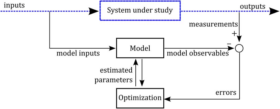
Figure 1 Scheme of the parameter identification process. A model structure has been defined to represent the dynamics of a system under study. Dashed lines represent the system (real world) and solid lines represent the virtual mathematical/numerical world. By an experimental protocol, dynamic measurements of some quantities characterizing the system behaviour have been collected. The model parameters are identified by an optimization algorithm that minimizes the model errors (distance between the measured quantities and the model observables).
The parameter identification problem is often an ill-posed problem (it is a problem whose solution is not unique). This characteristic is the result of different aspects related to model structure, experimental data and numerical algorithms (Walter and Pronzato, Reference Walter and Pronzato1997; Vargas-Villamil and Tedeschi, Reference Vargas-Villamil and Tedeschi2014). Ideally, we expect that the problem solution provides reliable numerical values of the parameters. In the following section, we discussed tools for tackling the parameter identification problem.
Structural identifiability
Once the structure of a model is fixed and before attempting a numerical estimation of the model parameters, we might want to know if we have chances of succeeding in estimating unique optimal values of the model parameters from a given experimental setup. As previously mentioned, the possibility of recovering uniquely the model parameters relates to the mathematical property of structural identifiability, which is addressed on the sole basis of the model structure within a hypothetical ideal experiment determined by a setting of model inputs (stimuli) and observable variables (measurements). In this theoretical framework, it is assumed that the model represents perfectly the system, the observables are noise-free, and the inputs can be chosen freely to provide a sufficient excitation on the model response.
The property of structural identifiability is independent of real experimental data and is determined as follows. Let M(p) be a fixed model structure with a set of parameters ${\bf p}\,{\equals}\,\left( {p_{1} , \cdots ,p_{{n_{{\rm p}} }} } \right)$
. M(p) describes the relationship between input variables and observables. Let us denote by M(p)=M(p*) the equality of the input–output behaviour of the model structure obtained for the two parameter sets p,p*. A parameter p
i
(i=1, … , n
p) is structurally identifiable if the equality M(p)=M(p*) implies that
${\bf p}\,{\equals}\,\left( {p_{1} , \cdots ,p_{{n_{{\rm p}} }} } \right)$
. M(p) describes the relationship between input variables and observables. Let us denote by M(p)=M(p*) the equality of the input–output behaviour of the model structure obtained for the two parameter sets p,p*. A parameter p
i
(i=1, … , n
p) is structurally identifiable if the equality M(p)=M(p*) implies that $p_{i} \,{\equals}\, p_{i}^{{\asterisk}} $
, that is
$p_{i} \,{\equals}\, p_{i}^{{\asterisk}} $
, that is
 $${\bf M}\left( {\bf p} \right)\,{\equals}\,{\bf M}\left( {{\bf p}^{{\rm {\asterisk}}} } \right)\Rightarrow p_{i} \,{\equals}\,p_{i}^{{\rm {\asterisk}}} $$
To perform the analysis of identifiability, the equality M(p)=M(p*) is translated into a set of equations in p. These equations can often be put in the form of a set of polynomial equations in p (parameterized by p*). If the resulting set of equations has a unique solution for the parameter p i , the parameter is said to be structurally globally identifiable. If the number of solutions for p i is finite, the parameter is structurally locally identifiable. If infinite solutions exist for p i , the parameter is nonidentifiable. A model is structurally globally (or locally) identifiable if all its parameters are structurally globally (or locally) identifiable. A model is nonidentifiable if at least one of its parameters is nonidentifiable. A mathematical rigorous definition of structural identifiability is given by Walter and Pronzato (Reference Walter and Pronzato1997).
Different mathematical methods exist for testing the structural identifiability of dynamic models. The tools involved include the Laplace transform, Taylor series, generating series, similarity transformation and differential algebra. The interested reader is referred to the dedicated literature (Carson et al., Reference Carson, Cobelli and Finkelstein1983; Walter and Pronzato, Reference Walter and Pronzato1996; Chis et al., Reference Chis, Villaverde, Banga and Balsa-Canto2011b; Raue et al., Reference Raue, Karlsson, Saccomani, Jirstrand and Timmer2014). In Supplementary Material S1, the Laplace transform, Taylor series expansion, and generating series methods are described.
To illustrate the notion of structural identifiability, consider the following model:
y=a·b·x. We assume a hypothetical experimental protocol where x, y are measured. It is straightforward to conclude that only the quantity a·b is uniquely identifiable, while the individual parameters a, b are nonidentifiable. Nonidentifiability might imply that the model is over-parameterized (see Table 1). In this trivial example, it is clear that the model can be defined by one parameter instead of two.
As mentioned in the Introduction, testing the identifiability of a model might turn out to be difficult, demanding expertise on mathematical technicalities (see Supplementary Material S1). It is not our objective to go into the details of such technicalities. Rather, we take a practitioner perspective capitalizing on the developments of several software tools. These tools facilitate identifiability analysis by the practitioner (who does not have necessarily extensive knowledge in identifiability theory). Some of the identifiability software are as follows.
DAISY (Differential Algebra for Identifiability of SYstems) (Bellu et al., Reference Bellu, Saccomani, Audoly and D’Angio2007) which is implemented in the symbolic language REDUCE, GenSSI (Generating Series for testing Structural Identifiability) (Chis et al., Reference Chis, Banga and Balsa-Canto2011a) implemented in Matlab® and the IdentifiabilityAnalysis application (Karlsson et al., Reference Karlsson, Anguelova and Jirstrand2012) implemented in Mathematica. All of these three toolbox are freely available. The identifiability methods used by DAISY and GenSSI are explicitly referred in their acronyms. The IdentifiabilityAnalysis application uses the exact arithmetic rank approach. Although DAISY and GenSSI perform global identifiability analysis, IdentifiabilityAnalysis performs local identifiability analysis, but has the advantage of allowing the analysis of complex models. Overall, the outcome of these toolboxes is a qualitative report that displays the parameters that are identifiable.
The relevance of identifiability
In the following, we discuss the relevance of the identifiability question by means of five case studies with different modelling objectives.
Case study 1: we would like to know if we have a chance of succeeding in estimating uniquely the parameters of our model
The aim pursued here is of a mathematical nature. We want to know if the parameter identification problem is well-posed. Let us consider the mathematical model proposed by Wood (Reference Wood1967) that describes the lactation curve in cattle. We will refer to this model as M W. In this model, the daily milk production by the mammary gland (y) is described by the following γ type algebraic equation
 $$y\left( t \right)\,{\equals}\,a \cdot t^{b} \cdot {\rm exp}\left( {{\minus}c \cdot t} \right)$$
where t is the time after calving and a, b, c are empirical parameters that determine the shape of the curve. M W is not an ODE model (although it can be transformed into an ODE by simply deriving in time equation (2)). Since M W is relatively simple, its identifiability can be assessed by inspection. Indeed, by taking logarithms in both sides of equation (2), we obtain
 $$\ln \,y\left( t \right)\,{\equals}\,\ln \,a{\plus}b \cdot \ln \,t{\minus}c \cdot t{\rm }$$
If continuous data of milk yield are available, it can be concluded that the model parameters are uniquely identifiable (Wood, Reference Wood1967) and thus the parameter identification problem is well-posed.
Case 2: we are interested in knowing the actual value of the model parameters because of their biological relevance
In some cases, we are content with providing a model that satisfactorily predicts a variable of interest without the need to address identifiability issues. However, if our modelling objective goes beyond the purely predictive scope and we aim to improve the understanding of the phenomena that govern the system under study, the situation changes. In this case, we can be interested in knowing the actual values of the model parameters. In mechanistic models (see Table 1 for a definition), the parameters are biologically meaningful and we may wish to identify them uniquely because of their relevance.
Let us consider the lactation curve model proposed by Dijkstra et al. (Reference Dijkstra, France, Dhanoa, Maas, Hanigan, Rook and Beever1997), that we will refer to as M D. In contrast to M W, M D was originally formulated as an ODE model. Both models have equivalent predictive capabilities (Friggens et al., Reference Friggens, Brun-Lafleur, Faverdin, Sauvant and Martin1999). In M D, the daily milk production is described by
 $${{{\rm d}y} \over {{\rm d}t}}\,{\equals}\,k_{1} \cdot {\rm exp}\left( {{\minus}k_{2} \cdot t} \right) \cdot y{\minus}k_{3} \cdot y,\,y\left( 0 \right)\,{\equals}\,y_{0} $$
with y 0 the initial condition of milk production. The parameter k 1 is the specific rate of secretory cell proliferation at parturition, k 2 a decay parameter that modulates the proliferation of secretory cells and k 3 a specific rate of cell death. The analytical solution of M D is
 $$y\left( t \right)\,{\equals}\,y_{0} \cdot {\rm exp}\left\{ {{{k_{1} } \over {k_{2} }} \cdot \left[ {1{\minus}{\rm exp}\left( {{\minus}k_{2} \cdot t} \right)} \right]{\minus}k_{3} \cdot t} \right\}{\rm }$$
For models with parameters that are biologically meaningful, the question of identifiability appears relevant and useful since knowing the actual value of the parameter can be of help for providing biological insight on the system under study. For example, we may wish to know unequivocally the specific rate of secretory cell proliferation at parturition (parameter k 1) of M D. For that, we tested the identifiability of M D in equation (4) with the DAISY toolbox; DAISY handles models described by polynomial equations. As M D has an exponential equation, the model was suitably manipulated to facilitate the identifiability analysis as follows. We include a new state variable x 1(t)=exp(−k 2·t), which results in the following ODEs
 $$\eqalignno{ {{{\rm d}y} \over {{\rm d}t}}\,{\equals}\, & k_{1} \cdot x_{1} \cdot y{\minus}k_{3} \cdot y,\,y\left( 0 \right)\,{\equals}\,y_{0} \cr &{{{\rm d}x_{1} } \over {{\rm d}t}}\,{\equals}\,{\minus}k_{2} \cdot x_{1} ,\,x_{1} \left( 0 \right)\,{\equals}\,1 $$
If the milk yield is measured, the model parameters are uniquely identifiable (see the DAISY output file in Table 2). The computation time for the identifiability testing was <1 s on an Intel processor of 3.20 GHz with 8.0 GB RAM.
Table 2 Output file of Differential Algebra for Identifiability of Systems (DAISY) resulting from the identifiability analysis of the lactation model of Dijkstra et al. (1997). The model was suitably manipulated to be expressed with polynomial equations (a requirement of DAISY). The model is structurally globally identifiable since the basis gi provides a unique solution for all the parameters
To enlarge the discussion about the cases where identifiability is relevant, we tackled in Supplementary Material S2, the identifiability analysis of a kinetic model of ruminal lipolysis and biohydrogentation under in vitro conditions (Moate et al., Reference Moate, Boston, Jenkins and Lean2008). This model has the potential to be used as primary scaffold for improving the mechanistic description of rumen fermentation in existing models where lipid metabolism is either represented in a simplified fashion (Baldwin et al., Reference Baldwin, Thornley and Beever1987; Mills et al., Reference Mills, Dijkstra, Bannink, Cammell, Kebreab and France2001) or not accounted for (Muñoz-Tamayo et al., Reference Muñoz-Tamayo, Giger-Reverdin and Sauvant2016).
Case 3: the model should predict unobserved variables
The theoretical framework of structural identifiability assumes perfect experimental data (noise-free and continuous in time). In addition, some hypotheses on the initial conditions of the state variables need to be assumed. Initial conditions can be assumed to be unknown or fixed. These assumptions have implications on the results of identifiability testing (Saccomani et al., Reference Saccomani, Audoly and D’Angio2003). We will use an example borrowed from Balsa-Canto and Banga (Reference Balsa-Canto and Banga2010), and further discussed by Villaverde and Barreiro (Reference Villaverde and Barreiro2016). Let us consider a system described perfectly by the following ODE model
 $$\eqalignno{ & {{{\rm d}x_{1} \left( t \right)} \over {{\rm d}t}}\,{\equals}\,p_{1} \cdot x_{1} \cdot x_{2} , \,x_{1} \left( 0 \right)\,{\equals}\,x_{{10}} \cr & {{{\rm d}x_{2} \left( t \right)} \over {{\rm d}t}}\,{\equals}\,p_{2} \cdot u,\,x_{2} \left( 0 \right)\,{\equals}\,x_{{20}} \cr &\,y_{1} \left( t \right)\,{\equals}\,x_{1} \left( t \right) $$
The model has two state variables (x 1, x 2) and one input (u). Note that the input can be time-variant (u(t)). For illustration purposes, we assume here that the input is known and constant over time. Only the state variable x 1 can be measured. This condition is represented in the definition of the observable variable y 1. The initial conditions are set by a hypothetical experimental protocol. By solving analytically the model equations in equation (7), we obtain the following equation for the model observable:
 $$y_{1} \left( t \right)\,{\equals}\,x_{{10}} \cdot {\rm exp}\left( {p_{1} \cdot x_{{20}} \cdot t{\plus}0.5 \cdot p_{1} \cdot p_{2} \cdot u \cdot t^{2} } \right)$$
Let us now assume that the initial conditions are set to x
10=1, x
20=0, which leads to $y_{1} \left( t \right)\,{\equals}\,{\rm exp}\left( {0.5 \cdot p_{1} \cdot p_{2} \cdot u \cdot t^{2} } \right)$
. It is clear that under these initial conditions, only the quantity p
1·p
2 can be recovered from the observable variable. Hence, we can conclude that the model is nonidentifiable (i.e. p
1, p
2 cannot be uniquely identified). This result implies that when performing the calibration, infinite solutions can be found which will make the calibration difficult.
$y_{1} \left( t \right)\,{\equals}\,{\rm exp}\left( {0.5 \cdot p_{1} \cdot p_{2} \cdot u \cdot t^{2} } \right)$
. It is clear that under these initial conditions, only the quantity p
1·p
2 can be recovered from the observable variable. Hence, we can conclude that the model is nonidentifiable (i.e. p
1, p
2 cannot be uniquely identified). This result implies that when performing the calibration, infinite solutions can be found which will make the calibration difficult.
Let us now assume that the model has the following true parameter values: p 1=1.0, p 2=2.0 and the input is u=1.0. By true parameters we refer to the ideal assumption that the model represents perfectly the system. In reality the true parameters are unknown. Now, under the hypothetical experimental conditions, any set of parameters fulfilling the condition p 1·p 2=2.0 is a solution of the parameter identification problem. Assume that noise-free data are available and that the optimization routine led to the following estimated parameters p 1=2.0, p 2=1.0. Note that the parameters fulfil the relationship p 1·p 2=2.0. To demonstrate the relevance of structural identifiability we compare the time series of x 1 and x 2 from the model simulation using the true parameters and the set of estimated parameters. This comparison was performed by using the original initial conditions of the hypothetical experimental protocol (x 10=1, x 20=0, Figure 2a) and an additional set of initial conditions (x 10=1, x 20=0.5, Figure 2b).
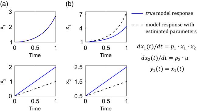
Figure 2 Relevance of structural identifiability analysis. The model response with the true values of parameters p 1=1.0, p 2=2.0 (continuous blue lines) is compared with the model response with parameters (p 1=2.0, p 2=1.0) obtained from a hypothetic calibration scenario (dashed black lines) with initial conditions x 10=1, x 20=0 (a), and where only x 1 can be measured ideally (noise free). Under these conditions, the model is nonidentifiable (only p 1·p 2 is identifiable). In (b), the initial conditions are x 10=1, x 20=0.5. The parameters estimated from the experimental conditions in (a) cannot provide accurate predictions under other experimental conditions.
From this example, the following conclusions can be drawn:
-
a. If our modelling objective is to predict the dynamics of x 1, we can think at first sight that the identifiability question is irrelevant because whatever estimated parameters we obtain, we will be able to predict x 1. This reasoning, however, needs to be taken with caution. If we constrained our modelling scope to the experimental protocol with initial conditions x 10=1, x 20=0, the question of identifiability is indeed irrelevant. As observed in the left top plot of Figure 2a, the response of the two models evaluated with the true and estimated set of parameters are identical and thus we will be content in finding a set of parameters such that p 1·p 2=2.0. However, if we are interested in enlarging the prediction capabilities of the model to a broader experimental context, the question of identifiability becomes relevant and necessary. We observe in the right top plot of Figure 2b that the model response with estimated parameters differs from the response with the true parameters. This result implies that any prediction of x 1 in a different experimental context from that used for the model calibration will be wrong.
-
b. If, in addition to predicting the dynamics of x 1, we are interested in predicting x 2, the identifiability question is of greater relevance. The two bottom plots illustrate that if structural identifiability cannot be guaranteed, the model predictions of x 2 will certainly be wrong.
The lack of identifiability of this model can easily be reversed. Indeed, by simply setting x 20>0, the parameters p 1, p 2 are uniquely identifiable. In Supplementary Material S1, we show the structural identifiability analysis of this model by using the Taylor series and the generating series methods. We also analysed the parameter identifiability of the model using DAISY. The identifiability analysis was performed in less than one second. This example stresses the importance of the design of an experimental protocol (including the initial conditions) for guaranteeing structural identifiability.
Case 4: we attempt to use our model for testing hypotheses that cannot be verified experimentally
In animal science, the lack of experimental data on key variables can lead to multiple model structures for representing the same process (Sauvant, Reference Sauvant1994). This multiplicity comes from the subjective nature of model construction that makes modelling similar to a form of art (Barnes, Reference Barnes1995). One of the powerful applications of mathematical modelling is that of providing a mean to address questions that are difficult to tackle experimentally. These applications include the opportunity of modelling abstract/theoretical variables that cannot be measured. We will illustrate this powerful role of models with the topic of nutrient partitioning. This issue is central in animal nutrition since the amount of nutrient that fuels a function (such as growth or lactation) is the basis for predicting nutrient requirements and develop feeding systems and recommendations.
Nutrient partitioning is regulated by two systems: a short-term system, namely homoeostatic system, and a long-term system, namely homeorhetic system (Sauvant, Reference Sauvant1994). Homoeostasis regulations consists of an ensemble of adaptation and survival functions of an individual, such as glycaemia regulation after a meal. Homeorhetic regulations correspond to the orchestrated hormonal changes that drive metabolism to support the succession of physiological states that favour species survival. An example of a homeorhetic regulation is the increase of body reserves mobilization in early lactation to support milk production.
Different approaches exist to represent homeorhetic control of nutrient partitioning (Friggens et al., Reference Friggens, Emmans and Veerkamp2013) but their common feature is the use of theoretical components to account for complex underlying mechanisms. These theoretical variables are used in models as proxy for translating the effects of mechanisms at underlying levels of organization. For instance, the concept of ‘theoretical hormones’ or ‘meta-hormones’ has been used to represent the driving forces of body reserves changes (Hanigan et al., Reference Hanigan, Rius, Kolver and Palliser2007). The concept of ‘priorities’ for life functions has been used to investigate dynamic trajectories of lactating ruminants (Puillet et al., Reference Puillet, Martin, Tichit and Sauvant2008; Martin and Sauvant, Reference Martin and Sauvant2010). All these conceptual elements are used to represent the result of complex mechanisms that control nutrient partitioning and that are not possible to measure experimentally. The incorporation of theoretical driving forces in animal science modelling has been useful to move forward in predicting animal responses to their nutritional environment; that is, coordinated responses of both body reserves and milk production in the dairy goat (Puillet et al., Reference Puillet, Martin, Tichit and Sauvant2008) and in the dairy cow (Martin and Sauvant, Reference Martin and Sauvant2010).
Let us consider in some detail the compartmental model developed by Puillet et al. (Reference Puillet, Martin, Tichit and Sauvant2008) to represent a homeorhetic regulatory system that controls body reserves changes and milk production across parity in dairy goats. Model equations, based on a system of priorities, are:
 $$\eqalignno{ &{{{\rm d}A\left( t \right)} \over {{\rm d}t}}\,{\equals}\, {\minus}k_{1} \cdot A, A\left( 0 \right)\,{\equals}\,A_{0} \cr &{{{\rm d}B\left( t \right)} \over {{\rm d}t}}\,{\equals}\,k_{1} \cdot A{\minus}k_{2} \cdot B, B\left( 0 \right)\,{\equals}\,B_{0} \cr &{{{\rm d}C\left( t \right)} \over {{\rm d}t}}\,{\equals}\,k_{2} \cdot B, {\rm }C\left( 0 \right)\,{\equals}\,C_{0} $$
where the state variables A, B, C represent, respectively, the priorities for body reserves mobilization, milk production and body reserves reconstitution. Simple mass-action kinetics (determined by the kinetic parameters k 1, k 2) are used to capture the major phases of body reserves changes throughout lactation process, represented as a transfer of priorities. Figure 3 displays the model schematics. At parturition, the priorities for using reserves and for producing milk are high. Then priority for body reserves mobilization decreases and, simultaneously, priority for milk production increases until it reaches a peak. This is followed by a shift in priority from milk production to body reserves reconstitution. The model structure has been constructed on biological basis. Indeed, the priority A follows an analogous dynamics to the body lipid mobilization dynamics (which can be indirectly assessed by plasma non-esterified fatty acids content), and the priority B follows an analogous dynamics to the observed dynamics of a lactation curve.
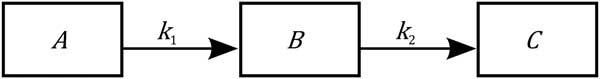
Figure 3 Schematics of the homeorhetic regulatory model of a dairy goat of Puillet et al. (Reference Puillet, Martin, Tichit and Sauvant2008). The compartments A, B, C are, respectively, the priorities for body reserves mobilization, milk production and body reserves reconstitution. The model describes the lactation process as a flow of substance moving through three successive compartments following mass-action kinetics (with the parameters k 1, k 2). The model structure follows a biological basis. For example, priority A follows an analogous dynamics to body lipid mobilization, and priority B follows an analogous dynamics to the lactation curve.
We tested the identifiability of the model in equation (9) with DAISY. The model parameters (k 1, k 2) are uniquely identifiable if at least two state variables are measured simultaneously. They are also uniquely identifiable if either B or C are measured and the initial conditions are known. If only A is measured, the model is nonidentifiable. The computation time for identifiability testing was <1 s.
It should be noted that the priorities described by the model are abstract variables that cannot be measured. In this case, the model construction is motivated by providing a conceptual and pertinent structure that concretizes biological hypothesis rather than producing a quantitative prediction tool. It was also constructed to overcome the existing difficulty of performing experiments to quantify homeorhetic mechanisms. As a consequence, the question of structural identifiability is in this case not relevant and does not preclude the models usefulness as a tool for understanding. Indeed, model simulations have provided useful information to analyse theoretical dynamics of phenotypic variables of interest such as milk production and body reserves.
With an academic motivation, let us analyse the hypothetical case where the priorities A, B, C of the model in equation (9) can be measured by an adequate experimental technique. This hypothetical case is here assumed to demonstrate the relevance that identifiability analysis can have for guiding experiment design. Suppose we plan to perform a series of experiments for estimating the model parameters with a limited budget of 10 €. The cost of measuring A, B and C is, respectively, 2 €, 8 € and 10 €. How to select what to measure? Well, given the critical situation of funding in research, we will be tempted to choose to measure only A and use the remaining 8 € in other projects. This decision is of course wrong, because measuring only A will not provide quality information for model calibration. Measuring either B or C will be adequate. If we measure only B, we will have 2 € to compensate our financial deficit. However, if we want to get the most out of the experiment, the wisest choice is to measure both A and B.
Let us now consider the following model and assume that it can be an alternative model of the regulatory model in equation (9).
 $$\eqalignno{ &{{{\rm d}A\left( t \right)} \over {{\rm d}t}}\,{\equals}\, {\minus}{{k_{1} } \over {k_{3} {\plus}A}} \cdot A \cdot B, A\left( 0 \right)\,{\equals}\,A_{0} \cr &{{{\rm d}B\left( t \right)} \over {{\rm d}t}}\,{\equals}\,{{k_{1} } \over {k_{3} {\plus}A}} \cdot A \cdot B{\minus}k_{2} \cdot B, B\left( 0 \right)\,{\equals}\,B_{0} \cr &{{{\rm d}C\left( t \right)} \over {{\rm d}t}}\,{\equals}\,k_{2} \cdot B, {\rm }C\left( 0 \right)\,{\equals}\,C_{0} $$
This model is more complex than the model in equation (9). First, it is nonlinear because the flux from A to B is described by a nonlinear function (Michaelis–Menten kinetics) instead of a first-order kinetics, and second, it has one additional parameter (k 3). We tested the identifiability of the model using DAISY, GenSSI and IdentifiabilityAnalysis. The computation time was <1 s in all the three toolboxes. In this case, the parameters of the model are identifiable if any of the state variables is measured. If only A is measured the model parameters are identifiable, which contrasts to the identifiability properties of the original model described by equation (9) (nonidentifiable if only A is measured). The result appears at first sight as counterintuitive, since in modelling practice complex models are often penalized. In the framework of structural identifiability, nonlinear models tend to be more identifiable than linear models (Walter and Pronzato, Reference Walter and Pronzato1996; Roper et al., Reference Roper, Saccomani and Vicini2010). In the previous example, adding a nonlinearity and a supplementary parameter help to improve the structural identifiability of the model. However, the increase of the number of parameters has, in general, a negative influence on the practical identifiability by rendering the model calibration harder, and increasing the risk of overfitting.
Case 5: what if in our modelling scenario the question of structural identifiability is relevant but our model is nonidentifiable?
As it was previously mentioned, the lack of experimental data on key variables imposes a particular challenge in the modelling task and can lead to various difficulties including the lack of structural identifiability. Models where the number of parameters is very high with respect to number of observables may lack of structural identifiability. Although, as demonstrated in the case study 4, we cannot affirm systemically that models with more parameters are less identifiable than models with less parameters. The identifiability depends on the model structure and on how the parameters appear in the observables. After this clarification, the lack of identifiability of mathematical models is not an uncommon scenario, and is often encountered in domains such as system biology. Then, what to do? One popular solution consists in capitalizing on existing knowledge by setting some parameters to known values reported in the literature. This strategy (expert guess) results in reducing the number of unknown parameters to be estimated and may favour the identifiability of the reduced parameter set. Caution should be paid in selecting parameters obtained from experimental conditions that are compatible to the case study. Parameter reduction can also be performed by grouping some of the model parameters (Schaber and Klipp, Reference Schaber and Klipp2011). A second solution is to design a new experiment that renders the model identifiable by selecting an adequate set of observables (Anguelova et al., Reference Anguelova, Karlsson and Jirstrand2012).
If after exhausting the above-mentioned alternatives the nonidentifaibility cannot be eliminated, this does not necessarily mean that our model is useless. First, the model construction requires the verbal hypotheses on the system under study to become specific and conceptually rigorous (Schaber and Klipp, Reference Schaber and Klipp2011). This conceptual step is central for gaining insight on the system behaviour, and pointing out the aspects that need to be deepened. Second, if our modelling purpose is to predict, we can assess numerically to what extend the lack of identifiability can impact model predictions. We can identify which set of variables of the model are the less sensitive to the actual values of the parameters (Gutenkunst et al., Reference Gutenkunst, Waterfall, Casey, Brown, Myers and Sethna2007) and which model predictions can be uniquely determined despite lack of identifiability (Cedersund, Reference Cedersund2012). We emphasized that the nonidentifiability of a model does not preclude its usefulness. A relevant example is the model of the circadian clock in Arabidopsis thaliana (Locke et al., Reference Locke, Millar and Turner2005). The model has 29 parameters, from which only 17 parameters are at least locally identifiable under certain stimuli (Chis et al., Reference Chis, Villaverde, Banga and Balsa-Canto2011b). Although its lack of identifiability, the model of Arabidopsis thaliana represents an important modelling contribution for enhancing understanding of the loops of genes that drive circadian locks in living organisms. By being aware of the lack of identifiability and by using adequate tools, nonidentifiable models can still be useful by providing both qualitative and quantitative information for gaining insight on system behaviour (Schaber and Klipp, Reference Schaber and Klipp2011; Cedersund, Reference Cedersund2012).
A brief summary about the relevance of identifiability discussed here is given in Table 3. To sum up, structural identifiability analysis remains desirable whenever feasible in the model calibration context, since it determines if the parameter identification problem has a unique solution when we have unlimited available data. Identifiability testing can provide guidelines for designing experiments and be useful for facilitating model simplification by identifying some potential over-parameterizations. Together, this information facilitates the model calibration step. Identifiability analysis is therefore relevant when (i) we are interested in the actual values of the model parameters, and (ii) we want to predict variables, in particular those that cannot be measured directly. Although structural identifiability is a desired property of a model, we clearly state that a nonidentifiable model can still be a useful model.
Table 3 Summary of the case studies for assessment the relevance of structural identifiability
In addition to the identifiability methods previously mentioned, identifiability analysis can also be performed numerically, for example, by using interval analysis (Braems et al., Reference Braems, Jaulin, Kieffer and Walter2001). Numerical approaches allow the computational complexity associated with identifiability methods based on algebraic manipulations of observable derivatives to be overcome. Indeed, when dealing with complex models, identifiability analysis may be impossible to perform even with the advanced software tools applied here, and recent developments (Villaverde et al., Reference Villaverde, Barreiro and Papachristodoulou2016), and thus the assessment of structural identifiability by numerical means is of great value. A very intuitive solution consists in using prior values of the model parameters for generating simulated data for a hypothetical experimental setup and perform the model calibration. By inspection, we can assess if the resulting parameter estimates are close to the priors values used for data generation. If this is this case, the model might be at least locally identifiable (Walter and Pronzato, Reference Walter and Pronzato1997). A more sophisticated solution is that of the profile likelihood approach (Raue et al., Reference Raue, Kreutz, Maiwald, Bachmann, Schilling, Klingmuller and Timmer2009) which provides a powerful numerical method for assessing structural and practical identifiability of high-dimension models.
On practical identifiability and optimal experiment design for parameter estimation
In the previous section, we mentioned that structural identifiability is a necessary condition for the well-posedness of the model calibration problem. However, structural identifiability does not guarantee the accuracy of the estimation and the quality of the model predictions (Carson et al., Reference Carson, Cobelli and Finkelstein1983). In practice, we aim to find accurate parameter estimates from experimental data. The actual accuracy of the parameter identification depends on the characteristics of the actual experimental data. The question to be addressed is: for a fixed model structure and given a set of experimental data, how accurate will be the estimated parameters? Data are always corrupted by noise, and are usually in short supply (although this situation is rapidly changing due to the progress of precision farming technologies). Hence, even if the model is structurally identifiable, the quality of the estimation can be poor, leading to parameter estimates that can even take values that are physically meaningless. Furthermore, there might exist many sets of parameter values that fit the data equally well, which can be troublesome for drawing biological-based conclusions as discussed by Boer et al. (Reference Boer, Butler, Stotzel, Te Pas, Veerkamp and Woelders2017) when addressing the parameter estimation of a bovine oestrous cycle model.
Tackling the accuracy of the parameter identification with respect to experimental data is the core of practical identifiability. To illustrate the notion of practical identifiability, let us consider the model y=a·x 1+b·x 2 and assume that the variables x 1, x 2, y can be measured. The parameters a, b are structurally identifiable. Now, consider that experimental data are available and that x 1, x 2, are proportional (i.e. x 2=c·x 1). With these data, the parameters a, b are not practically identifiable. The only quantity that is practically identifiable is a+b·c. The parameter estimates under these experimental conditions will not be accurate. Accuracy of the parameter estimation is related to parameter uncertainty (high accuracy implies low uncertainty) and is assessed by the computation of the confidence intervals of the parameter estimates. Large confidence intervals imply low reliability on the parameter estimates (practical unidentifiability).
One classical approach for determining the confidence intervals of the parameter estimates is via the computation of the Fisher Information Matrix (FIM). In Supplementary Material S3, we recall the principles of this classical approach and introduce some aspects of OED for parameter estimation. The goal of OED is to find, under a set of constraints, an experiment setup that allows an accurate estimation of the model parameters (which translates in small confidence intervals). To illustrate the power of OED, consider the curve lactation model M D in equation (4). The OED problem is defined with a prior nominal parameter set (extracted from literature or experimental data). Let us assume that these nominal values are k 1=0.1, k 2=0.15, k 3=0.005, and that the initial condition of yield milk is y 0=10 with t 0 =0.1 day. We aim to find three sampling times along 100 days that provide high informative content for estimating the model parameters accurately. For that, we defined an OED problem in which the optimal sampling times were found by maximizing the determinant of the FIM. Maximizing the determinant of the FIM implies minimizing the volume of the confidence intervals (see Supplementary Material S3). The FIM was obtained by symbolic manipulation using the Matlab® Toolbox IDEAS (Muñoz-Tamayo et al., Reference Muñoz-Tamayo, Laroche, Leclerc and Walter2009), which is freely available at http://genome.jouy.inra.fr/logiciels/IDEAS. The OED problem was solved using the Nelder–Mead Simplex method implemented in Matlab®.
The optimal sampling times were: t 0 =0.1 days, t 1=7.5 days, t 2=29 days, t 3=100 days. For comparison, we calculated the confidence intervals obtained from an equidistant sampling time setup (t 0 =0.1 days, t 1=33.4 days, t 2=66.7 days, t 3=100 days). Figure 4 displays the obtained optimal sampling times, together with the sampling times from the equidistant strategy. Table 4 shows the comparative results. Optimal sampling times obtained from OED provide substantially a better accuracy of the estimation than equidistant sampling times. For k 1, k 2, the standard deviations from the OED are only 5% of the standard deviations provided by the equidistant sampling setup. For k 3, the standard deviation from the OED is 50% of that obtained with the equidistant sampling setup.
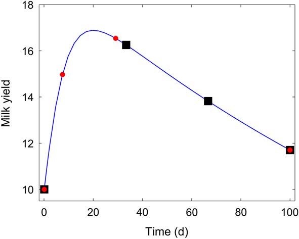
Figure 4 Lactation model of Dijkstra et al. (Reference Dijkstra, France, Dhanoa, Maas, Hanigan, Rook and Beever1997). Equidistant sampling times (■), v. sampling times obtained from optimal experiment design (![]() ).
).
Table 4 Accuracy of the parameter estimates of the lactation model of Dijkstra et al. (Reference Dijkstra, France, Dhanoa, Maas, Hanigan, Rook and Beever1997) for an equidistant sampling strategy and a sampling strategy obtained by optimal experiment design (OED)
This example illustrates the capabilities of OED and the interest of incorporating this tool into our modelling practice when data have not been collected yet. Optimal experiment design allows maximum exploitation of experimental data for model calibration, and avoid pitfalls from applying traditional experiment designs without cautious analysis. In fact, it is common practice to use factorial designs for defining an experimental setup. If the levels are not chosen adequately, the factorial design can lead to practical identifiability problems such a singular FIM (see Muñoz-Tamayo et al., Reference Muñoz-Tamayo, Martinon, Bougaran, Mairet and Bernard2014 for an illustrative example). If this occurs, the reliability of the parameter estimates cannot be assessed given that confidence intervals computation requires the FIM to be invertible (see Supplementary Material S3).
It goes without saying that the identification of model parameters is a very challenging problem, where difficulties are encountered even for models of moderate complexity. In the case of a complex model, one may wonder, however, about the practical relevance of providing a result about the identifiability of the model, given that identifying the parameters of the model from actual noisy data is already extremely difficult. In this respect, by studying the parameter sensitivities of a collection of 17 models of biological systems, Gutenkunst et al. (Reference Gutenkunst, Waterfall, Casey, Brown, Myers and Sethna2007) have elaborated the concept of sloppiness, that establishes that some parameters (sloppy) can change by orders of magnitude without affecting significantly the model output. Sloppiness is related to the condition number of the FIM (Supplementary Material S3) and results from high differences between the eigenvalues of the FIM. The parameter identification of a sloppy model data suffers from high uncertainty as a result of a singular (ill-conditioned) FIM. The authors claimed that sloppiness is a universal property of systems biology models and suggest that modellers should focus on predictions rather than on identifying the actual values of the model parameters. Given this work, it may seem tempting to desist from any efforts to look for an accurate parameter identification. Nevertheless, the notion of sloppiness has been subject of debate and its value as conceptual tool has been questioned. In the comprehensive work of Chis et al. (Reference Chis, Banga and Balsa-Canto2016), it has been demonstrated that sloppy models can be identifiable and that OED can substantially improve the practical identifiability of models, even if they are complex. Chis et al. (Reference Chis, Banga and Balsa-Canto2016) suggested that OED should be performed on the basis of classical criteria such as maximizing the determinant of the FIM instead of looking at minimizing model sloppiness. Accordingly, addressing parameter identifiability in complex models is not a hopeless quest when the adequate tools are deployed.
Conclusions
This article was centred on introducing and discussing the mathematical tool of structural identifiability analysis, which has been seldom applied in animal science modelling. This lack of pervasiveness in our domain is probably due to the mathematical technicalities which identifiability analysis relies on. These technicalities are beyond the academic background in animal science. However, this hurdle can be overcome by adopting a practitioner perspective and capitalizing on existing dedicated identifiability software that should facilitate the application of identifiability analysis in our domain. By using illustrative examples, we attempted to open a window towards the discovery of a powerful tool for model construction and experiment design when the identifiability question is relevant. Overall, identifiability analysis is relevant when the purpose of the model construction is the prediction of variables that cannot be measured, and when we are interested in knowing the actual value of the model parameters. Finally, the success to getting the most out of structural identifiability analysis in animal science modelling relies on a constructive dialog between experimenters and modellers.
Acknowledgements
The authors would like to thank the developers of the identifiability toolboxes DAISY (Bellu et al., Reference Bellu, Saccomani, Audoly and D’Angio2007), GenSSI (Chis et al., Reference Chis, Banga and Balsa-Canto2011a) and IdentifiabilityAnalysis (Karlsson et al., Reference Karlsson, Anguelova and Jirstrand2012) for rendering their software freely available and favouring Open Science. Many thanks to Dr Maria Pia Saccomani (University of Padova, Italy) for helpful insights on the use of DAISY. The authors thank Nicolas Friggens (INRA-AgroParisTech, France) for his critical comments on the manuscript. R.M.T. is indebted to Éric Walter for his rigorous and provocative explanations on the fascinating subject of parameter identification.
Supplementary material
To view supplementary material for this article, please visit https://doi.org/10.1017/S1751731117002774


