


1. Introduction
Granular materials are ubiquitous in natural and engineering systems, such as debris flows, landslides, fresh concrete and fissured rocks. Understanding the constitutive behaviour of granular media is significant for solving problems in, among others, civil engineering, chemical engineering and pharmaceutical engineering. Progress has been made since the proposal of Bagnold rheology (Bagnold Reference Bagnold1954), where both normal and shear stresses are proportional to  $f(\phi _s)\rho _p\dot {\gamma }^{2}d^2$, and the $\mu (I)$ rheology (MiDi Reference MiDi2004; Jop, Forterre & Pouliquen Reference Jop, Forterre and Pouliquen2006; Pouliquen et al. Reference Pouliquen, Cassar, Jop, Forterre and Nicolas2006), where the effective frictional coefficient, $\mu = \tau /\sigma _n$, can be expressed as a function of the inertial number, $I = \dot {\gamma }d/\sqrt {\sigma _n/\rho _p}$ (where $f(\phi _s)$ is a function of the solid fraction $\phi _s$, $\rho _p$ is the particle density, $\dot {\gamma }$ is the shear rate, $d$ is the average particle size, $\tau$ is the shear stress and $\sigma _n$ is the pressure).
With the successful characterization of dry granular systems in non-transient states, granular column collapses were proposed to investigate the transient behaviour and to relate granular flows to natural geophysical flows, such as pyroclastic flows and landslides (Roche et al. Reference Roche, Gilbertson, Phillips and Sparks2002; Lacaze & Kerswell Reference Lacaze and Kerswell2009). Lube et al. (Reference Lube, Huppert, Sparks and Hallworth2004) and Lajeunesse, Monnier & Homsy (Reference Lajeunesse, Monnier and Homsy2005) tested the collapse morphology and kinematics of dry granular column collapses and concluded a power-law relationship between the initial aspect ratio,  $\alpha = H_i/R_i$, and the relative run-out distance, $\mathcal {R}=(R_{\infty } - R_i)/R_i$, where $H_i$ is the initial height of the column, $R_i$ is the initial column radius and $R_{\infty }$ is the final run-out radius after the column collapse. Based on the $\mathcal {R}(\alpha )$ relationship, a critical aspect ratio, $\alpha _c$, was observed to divide granular column collapses into two regimes: (1) when $\alpha < \alpha _c$, $\mathcal {R}$ is approximately proportional to $\alpha$ and (2) when $\alpha > \alpha _c$, $\mathcal {R}$ approximately scales with $\alpha ^{0.5}$ (Lube et al. Reference Lube, Huppert, Sparks and Hallworth2004, Reference Lube, Huppert, Sparks and Freundt2005; Thompson & Huppert Reference Thompson and Huppert2007). Zenit (Reference Zenit2005) performed discrete element method (DEM) simulations of two-dimensional granular column collapses, and confirmed that the shape of the final deposition was mainly determined by the initial aspect ratio. Staron & Hinch (Reference Staron and Hinch2005, Reference Staron and Hinch2007) further investigated two-dimensional granular column collapses with the DEM, and found that the interparticle frictional coefficient played an important role in the run-out distance, but did not quantify such frictional effects. Previous research also studied the complexity of granular column collapses when the system was subjected to different realistic conditions, such as particle size polydispersity (Cabrera & Estrada Reference Cabrera and Estrada2019; Martinez et al. Reference Martinez, Tamburrino, Casis and Ferrer2022), fluid saturation or immersion (Rondon, Pouliquen & Aussillous Reference Rondon, Pouliquen and Aussillous2011; Fern & Soga Reference Fern and Soga2017; Bougouin, Lacaze & Bonometti Reference Bougouin, Lacaze and Bonometti2019), complex particle shapes (Zhang et al. Reference Zhang, Yin, Wu and Jin2018) and erodible boundaries (Wu, Wang & Li Reference Wu, Wang and Li2021). However, no matter how complex the granular system was, the interparticle friction was often set constant and unique.
To account for the influence of both the interparticle friction and boundary friction, Man et al. (Reference Man, Huppert, Li and Galindo-Torres2021a) proposed an effective aspect ratio,
 \begin{equation} \alpha_{eff} = \alpha\sqrt{1/(\mu_w + \beta\mu_p) }, \end{equation}
based on a dimensional analysis, where  $\mu _w$ is the frictional coefficient between particles and the bottom plate, $\mu _p$ is the frictional coefficient between contacting particle pairs and $\beta$ is a fitting parameter, and later linked $\alpha _{eff}$ to the ratio between inertial effect and frictional resistance existing in granular systems during collapses. Thus, increasing the frictional coefficient increases the general frictional effect and decreases $\alpha _{{eff}}$. Similar to studies of Warnett et al. (Reference Warnett, Denissenko, Thomas, Kiraci and Williams2014) and Cabrera & Estrada (Reference Cabrera and Estrada2019), Man et al. (Reference Man, Huppert, Li and Galindo-Torres2021b, Reference Man, Huppert, Zhang and Galindo-Torres2022) also observed the size effect of granular column collapses but further related the size effect to finite-size scaling and characterized the influence of cross-section shapes using the finite-size scaling analysis, so that the size effect of granular column collapses can be quantified as
 \begin{equation} \mathcal{R} = \left({R_i}/{d}\right)^{-\beta_1/\nu}\mathcal{F}_r[(\alpha_{{eff}}-\alpha_{c\infty})\left({R_i}/{d}\right)^{1/\nu}] , \end{equation}
where  $\mathcal {F}_r[\cdot ]$ is a scaling function, scaling parameters $\nu = 1.39\pm 0.14$ and $\beta _1 = 0.28\pm 0.04$ are obtained to best collapse all the data and $\alpha _{c\infty }$ is the transitional effective aspect ratio when the system size goes to infinity. The influence of friction effects on granular column collapses resembled the friction-dependent rheology we proposed earlier (Man et al. Reference Man, Zhang, Ge, Galindo-Torres and Hill2023), where the frictional rheology depended on a frictional number, $\mathcal {M}$, which was also a ratio between inertial effects and frictional resistance.
However, no granular assembly in nature constitutes only one species of grains. A granular mixture may involve particles with different degrees of roughness and different angularities, which result in different interparticle frictional coefficients. We have confirmed the influence of frictional coefficient in our previous studies (Man et al. Reference Man, Huppert, Li and Galindo-Torres2021a, Reference Man, Zhang, Ge, Galindo-Torres and Hill2023), but have not yet explored the condition when a granular system contains particles with different friction properties. In this paper, we aim to address this issue by introducing a bi-frictional granular mixture, where the system includes two species of particles, Grain 1 and Grain 2, with different interparticle frictional coefficients, to investigate the mixing effect associated with granular column collapses using the DEM. This paper is organized as follows. In § 2, we provide a set of experimental examples to show the influence of mixing particles with different frictional coefficients. In § 3, we introduce both the DEM model and the simulation set-up, and define essential parameters. We then elaborate the simulation results and provide several discussions in § 4 to illustrate and quantify the mixing effect of bi-frictional systems, before providing some concluding remarks in § 5.
2. Experimental set-up and results
To experimentally verify the friction dependency of granular column collapses, we acquired two different type of particles. Grain 1 is irregular-shaped glass particles with diameter,  $d_1$, ranging from 1 to 3 mm (diameter range is obtained from sieve tests) and particle density, $\rho _1$, being approximately equal to 2.678 g cm $^{-3}$. Grain 2 is river sand particles with diameter, $d_2$, also ranging from 1 to 3 mm and particle density $\rho _2\approx 2.664\,{\rm g}\,{\rm cm}^{-3}$. We used a transparent plastic cylindrical tube to form the initial granular column, and the initial radius of tested granular columns was 23 mm. We varied the amount of granular materials poured into the cylindrical tube to achieve different initial packing heights ranging from $\approx 3$ to $\approx 146$ mm and resulting in the initial aspect ratio, $\alpha$, ranging from 0.13 to 6.34. Before each test, we used electrostatic-removal spray on the plastic tube, and no tribo-electric effect has been observed in these experiments. After placing particles into the cylindrical tube, we measured the initial height of the granular packing, $H_i$. Particles were dropped in from the top of the tube so that the initial condition resembled a randomly loose packing of the granular system. Then, the tube was manually lifted to release all the particles to form a granular pile. We measured the final radius of the sand pile in eight different directions and took their average as the final run-out distance, $R_{\infty }$. Then, the relationship between the initial aspect ratio, $\alpha$, and the normalized run-out distance, $\mathcal {R}$, can be obtained accordingly.
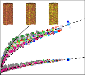
Three sets of experiments were performed in this study: (1) 100 % glass particles; (2) 100 % sand particles; and (3) 50 % glass + 50 % sand particles. In figure 1(a), we show the initial state and the final deposition of a simulation of 100 % glass particles. We can see that the glass particles have irregular shapes that resemble the shape of river sand. The initial height was 50 mm and the final run-out distance was approximately 78 mm. In figure 1(b), we show both the initial and final configurations of an experiment with 100 % river sand particles. The initial height was also 50 mm and the final run-out distance was approximately 68 mm. Figure 1(c) shows an example of mixing glass and sand. The mass ratio between two types of particles was  $1:1$. Given their similar density, the volume ratio was also approximately $1:1$. In figure 1(c), the initial height was 50 mm and the final run-out distance was approximately 75 mm.

Figure 1. Initial configurations and final depositions of granular column collapses of (a) 100 % irregular-shaped glass particles, (b) 100 % sand particles and (c) 50 % glass particles + 50 % sand particles. The cylindrical radius is 23 mm and the initial height in the figure is approximately 50 mm.
As shown in figure 1, changing the mixing ratio affects the final run-out distance. Thus, replacing part of the sand particles with glass particles improves the mobility of the granular mixture. We further tested columns with different initial heights and plot the relationship between  $\mathcal {R}$ and $\alpha$ in figure 2. In figure 2, the $x$ axis is $\alpha$ instead of $\alpha _{{eff}}$ because we do not have clear information about the frictional coefficient between particles during experiments. As we increase the percentage of the glass particles in the mixture, the relative run-out distance becomes larger. The experimental results agreed with our expectation, and implied that we should develop a method to quantify such mixing effect. However, since material properties in experiments are difficult to be determined and the initial packing is difficult to be reconstructed in a DEM environment, no comparison between experiments and simulations has been performed.

Figure 2. Experimental results of the relationship between the initial aspect ratio,  $\alpha$, and the relative run-out distance, $\mathcal {R}$.
Our analyses of experimental results are based on the assumption that sand particles are generally rougher than glass particles, hence having larger frictional coefficient. To verify this assumption, we need more concrete experimental results rather than only using our physical intuition. It is difficult to directly test the frictional coefficient between particles (Foerster et al. Reference Foerster, Louge, Chang and Allia1994; Lorenz, Tuozzolo & Louge Reference Lorenz, Tuozzolo and Louge1997). Thus, we choose to test the frictional coefficient between particles and different types of bottom plates. We build up the friction test platform using only LEGO $\circledR$ blocks, a plastic (PMMA) plate, a digital protractor, 80 g cm $^{-2}$ multi-purpose copypaper and two types of sandpapers, as shown in figure 3(a). We use LEGO $\circledR$ blocks to form a testing cart, where we could place testing particles beneath the cart to form several non-rolling particle ‘feet’ (figure 3b,c), so that the testing cart can only contact the bottom plate with its non-rolling particle feet. The non-rolling particle feet are arranged symmetrically to make the system more balanced and stable. The bottom plate is constructed by covering the PMMA plate with different basal materials, e.g. multi-purpose papers and sandpapers. We place the testing cart with granular feet onto certain basal plates of different materials (we make sure the basal materials are glued firmly onto the protractor) and lift one end of the plate until the testing cart starts to move. Since the testing plate was placed on a digital protractor, we could easily measure the inclined angle, $\theta _s$, when the cart starts to move. Thus, the tested frictional coefficient between target granular materials and the basal materials is calculated as $\mu _{pb} = \tan (\theta _s)$. We present friction test results of the average frictional coefficient and the standard deviation in table 1, where we measure frictional coefficients using a smooth PMMA plate, 80 g cm $^{-2}$ multi-purpose paper, P400 sandpaper and P800 sandpaper (smoother than P400 sandpapers). Generally, the average frictional coefficients of glass particles on different base materials are smaller than those of sand particles.

Figure 3. Experimental set-up for measuring the frictional coefficient between sand or glass particles and different basal materials.
Table 1. Frictional coefficients (average  $\pm$ standard deviation) between experimental particles and different types of bottom plates, $\mu _{pb}$.

We have to note that experimental results cannot confirm the influence of mixing frictions and quantify its influence. On the one hand, we merely show that sand particles are generally rougher than glass particles. On the other hand, smaller frictional coefficients lead to denser initial packing. For the same initial aspect ratio, glass particle packing often has a larger number of particles due to the denser packing condition, which may result in larger run-out distance in the end. In this study, we did not include a comparison between experiments and corresponding simulations because some material properties, e.g. real interparticle frictional coefficient, different particle shapes and coefficient of restitution, are difficult to obtain. Experimental results alone already fulfil our goal to illustrate the possible influence of mixing particles with different frictional properties. After showing the evidence of the influence of mixing particles with different frictional coefficient, we naturally move to simulation tools so that we can control the parameters much more easily.
3. Simulations
3.1. Governing equations
In this study, we performed simulations with the DEM (Galindo-Torres & Pedroso Reference Galindo-Torres and Pedroso2010) to test the collapse of granular columns with different frictional coefficients, which allowed us to easily and specifically control certain parameters and to extract particle-scale data from the system. We use Voronoi-based sphero-polyhedral particles in our simulations. The sphero-polyhedral method was initially introduced by Pournin & Liebling (Reference Pournin and Liebling2005) for the simulation of complex-shaped DEM particles. A sphero-polyhedron is a polyhedron that has been eroded and then dilated by a spherical element. The result is a polyhedron of similar dimensions but with rounded corners.
The advantage of the sphero-polyhedral technique is its easy and efficient definition of contact relationships among particles. When we calculate the contact force between adjacent particles, we can directly use the contact between their dilating spheres. Then, the contact calculation of complex-shaped particles is transformed into the contact between spheres. For example, we consider the contact between two generic particles named  $P_1$ and $P_2$. Particle $P_1$ has geometric features, such as a set of vertices $\{V_{1}^i\}$, edges $\{E_{1}^j\}$ and faces $\{F_{1}^k\}$. Particle $P_2$ also has geometric features, such as a set of vertices $\{V_{2}^i\}$, edges $\{E_{2}^j\}$ and faces $\{F_{2}^k\}$. Thus, a particle is defined as a polyhedron, i.e. a set of vertices, edges and faces, where each one of these geometrical features is dilated by a sphere. For simplicity, we denote the set of all the geometric features of $P_1$ and $P_2$ as $\{G_{1}^i\}$ and $\{G_{2}^j\}$. Then, we can calculate the distances between $\{G_{1}^i\}$ and $\{G_{2}^j\}$ as
 \begin{equation} \text{dist}(G_1^i,G_2^j) = \min(\text{dist}(\boldsymbol{X}_1^i,\boldsymbol{X}_1^j)), \end{equation}
where  $\boldsymbol {X}_1^i$ is a three-dimensional vector of points that belongs to the set $G_1^i$ and $\boldsymbol {X}_2^j$ is a three-dimensional vector of points that belongs to the set $G_2^j$. This means that the distance for two geometric features is the minimum Euclidean distance assigned to two points belonging to them.
Since both particles are dilated by their sphero-radii  $R_1$ and $R_2$, a contact is confirmed when the distance between the two geometric features is less than the sum of the corresponding radii used in the sweeping stage, i.e.
 \begin{equation} \text{dist}(G_1^i,G_2^j) < R_1+R_2, \end{equation}
and the corresponding contact overlap  $\delta _n$ can be calculated accordingly. Thus, the advantage of the sphero-polyhedral technique becomes evident since this definition is similar to that for the contact law of two spheres (Belheine et al. Reference Belheine, Plassiard, Donzé, Darve and Seridi2009). For each confirmed contact, we implement a Hookean contact model with energy dissipation to calculate the interactions between particles. At each time step, the overlap between adjacent particles, $\delta _n$, is checked and the normal contact force can be calculated using
 \begin{equation} \boldsymbol{F}_n ={-}K_n\delta_n\hat{\boldsymbol{n}} - m_e\gamma_{n}\boldsymbol{v}_n, \end{equation}
where  $K_n$ is the normal stiffness characterizing the deformation of the material, $\hat {\boldsymbol{n}}$ is defined as the normal unit vector at the plane of contact, $\boldsymbol {v}_n$ is the relative normal velocity between particles, $m_e = 0.5(1/m_1 + 1/m_2)$ is the reduced mass of the contacting particle pair, $m_1$ and $m_2$ are masses of contacting particles, respectively, and $\gamma _n$ is the normal energy dissipation constant, which depends on the coefficient of restitution $e$ as (Alonso-Marroquín et al. Reference Alonso-Marroquín, Ramírez-Gómez, González-Montellano, Balaam, Hanaor, Flores-Johnson, Gan, Chen and Shen2013; Galindo-Torres, Zhang & Krabbenhoft Reference Galindo-Torres, Zhang and Krabbenhoft2018)
 \begin{equation} e =
\exp\begin{pmatrix}-\displaystyle\frac{\gamma_n}{2}
\frac{\rm \pi}{\sqrt{\dfrac{K_n}{m_e} -
\left(\dfrac{\gamma_n}{2}\right)^2}}\end{pmatrix}. \end{equation}
\begin{equation} e =
\exp\begin{pmatrix}-\displaystyle\frac{\gamma_n}{2}
\frac{\rm \pi}{\sqrt{\dfrac{K_n}{m_e} -
\left(\dfrac{\gamma_n}{2}\right)^2}}\end{pmatrix}. \end{equation}
The tangential contact forces between contacting particles were calculated by keeping track of the tangential relative displacement  $\boldsymbol {\xi } = \int \boldsymbol {v}_t\,{\rm d}t$. Thus, the tangential contact forces follow
 \begin{equation} \boldsymbol{F}_t ={-}\min\left(|K_t\boldsymbol{\xi}|,\ \mu_p |\boldsymbol{F}_n|\right)\hat{\boldsymbol{t}}, \end{equation}
where  $K_t$ is the tangential stiffness, $\hat {\boldsymbol{t}}$ is the tangential vector in the contact plane and parallel to the tangential relative velocity, $\boldsymbol {v}_t$, and $\mu _p$ is the frictional coefficient between contacting particles and can be replaced by the frictional coefficient between the particles and the bottom boundary, $\mu _w$, while calculating the particle–boundary interactions. In this study, since we use Voronoi-based particles, no rolling resistance is needed. The motion of particles is then calculated by stepwise resolution of Newton's second law with the normal and contact forces mentioned before, so that
 $$\begin{gather} m_p\frac{\text{d}^2\boldsymbol{X}_p}{{\rm d}t^2} = \sum_c^{N_c}( \boldsymbol{F}_n^{pc} + \boldsymbol{F}_t^{pc} ) , \end{gather}$$
 $$\begin{gather}\frac{\text{d}}{\text{d}t}(\boldsymbol{I}_p \boldsymbol\omega_p) = \boldsymbol{T}_t, \end{gather}$$
where  $\boldsymbol {X}_p$ is the position vector of a particle, $m_p$ is the mass of a particle, $N_c$ is the number of contacts, $\boldsymbol {F}_n^{pc}$ and $\boldsymbol {F}_n^{pc}$ are normal and tangential contact force vectors acting from the contact point to the particle, $\boldsymbol {I}_p$ is the tensor of the moment of inertia of the particle, $\boldsymbol \omega _p$ is the angular velocity vector of the particle and $\boldsymbol {T}_t$ is the total torque subjected on the particle.
In the DEM simulation, we solve the governing equations of this classical interacting  $N$-body system using the velocity-Verlet method (Scherer Reference Scherer2017). The same neighbour detection and force calculation algorithms have already been discussed and validated in previous studies (Galindo-Torres & Pedroso Reference Galindo-Torres and Pedroso2010; Man et al. Reference Man, Huppert, Li and Galindo-Torres2021a), and the presented DEM formulation has been validated before with experimental data (Belheine et al. Reference Belheine, Plassiard, Donzé, Darve and Seridi2009; Cabrejos-Hurtado, Galindo Torres & Pedroso Reference Cabrejos-Hurtado, Galindo Torres and Pedroso2016) and is included in the MechSys open source multi-physics simulation library (Galindo-Torres Reference Galindo-Torres2013).
3.2. Simulation set-up
We performed simulations of the granular column collapses with Voronoi-based sphero-polyhedra (Galindo-Torres & Pedroso Reference Galindo-Torres and Pedroso2010). We note that the shape of particles could significantly influence the deposition morphology. In this study, we focus on using Voronoi-based particles so that the particles in the simulation are similar to sand particles. The detailed influence of particle shapes on the granular column collapses will be further explored in the future. In a simulation, we first generate Voronoi-based particle packing in a designed cylindrical domain of height  $H_i$ and radius $R_i = 2.5$ cm (figure 4). The number of particles within one unit length (1.0 cm) is five, so the average particle size is $\approx 2$ mm. Particles were packed within a column of radius $R_i$ equal to 2.5 cm and varying heights $H_i$ leading to cases of different initial aspect ratio. Then, 20 % of the sphero-polyhedron particles were removed to form a packing with a solid fraction of $\phi _s = 0.8$. We note that, in this simulation, we first construct a three-dimensional Voronoi system in the designed space so that each Voronoi cell is a discrete element particle. As a result, before removing 20 % of particles, the initial DEM packing has a solid fraction of 1. Height $H_i$ varies from 1 to 40 cm. In the simulations of Voronoi-based particles, the number of particles varied from approximately 1900 to approximately 68 500. The initial state of the granular column resembles a fissured rock with initial solid fraction $\phi _s = 0.8$. Then, we removed the cylindrical tube in the simulation and let grains flow downward freely with gravitational acceleration $g = 981\,{\rm cm}\,{\rm s}^{-2}$ (figure 4). Figure 4 shows the behaviour of a granular column from the initial state to the final deposition state. Each row of figure 4 represents a granular column with distinct mixing ratio of Grain 1 and Grain 2 (Grain 1 and Grain 2 only differ in their frictional properties). In the end, a cone-like pile of granular material with packing height, $H_{\infty }$, and average packing radius, $R_{\infty }$, will form.

Figure 4. Simulation set-up and collapse behaviours of systems with different mixing ratios. Red particles represent Grain 1 and yellow particles represent Grain 2. We cut one quarter of the granular assembly to show the inside of the system.
We implemented the Hookean contact model (elaborated in § 3.1) with energy dissipation and restitution coefficient  $e = 0.1$ to calculate the interactions between particles as described in the previous section. A relatively low value of $e$ was chosen to represent the rough surface of particles in real conditions (Li et al. Reference Li, Dong, Jiang, Li and Shang2020). We introduce two species of Voronoi-based particles in a system, where frictional properties of Grain 1 and Grain 2 are set separately. The frictional coefficient of the contact between Grain 1 and Grain 1, $\mu _{11}$, varies from 0.1 to 0.8. Similarly, we vary the frictional coefficient of the contact between Grain 2 and Grain 2, $\mu _{22}$, from 0.1 to 0.8. The frictional coefficient between Grain 1 and Grain 2 is then calculated as
 \begin{equation} \mu_{12} = \frac{2\mu_{11}\mu_{22}}{\mu_{11} + \mu_{22}}. \end{equation}
 Simulations were conducted with varied initial aspect ratios,  $\alpha$, between 0.4 and 16, varied mixing ratios where the percentage of Grain 2 varies from 10 % to 50 % and a constant particle–boundary frictional coefficient, $\mu _w = 0.4$, which is the same for both Grain 1 and Grain 2. Based on these simulations we obtained the run-out behaviour and deposition morphology for different conditions. We provide three movies as supplementary material available at https://doi.org/10.1017/jfm.2023.217 to show granular column collapses of systems with different mixing ratios ( $\mu _{11} = 0.4$ and $\mu _{22} = 0.2$). In these movies, different from figure 4, Grain 1 is coloured yellow and Grain 2 is coloured red.
4. Results and discussion
4.1. Flow behaviour
Generally, based on the propagation velocity of the front, a granular column collapse can be divided into three stages: (1) the acceleration stage, (2) the steady-propagating stage and (3) the deceleration stage. In figures 5–7, we measure the front position and the average kinetic energy for three sets of simulations and plot them against the collapse time. These three sets of simulations have different mixing ratios, but the same frictional coefficients ( $\mu _{11} = 0.1$, $\mu _{22} = 0.4$). The resulting front positions behave similarly among the three sets of simulations. As we increase the initial height of the granular column, the time when the granular flow stops varies from case to case. Columns with larger initial height can travel for longer time, since they need more time to dissipate the stored potential energy. We hypothesize that there may exist a relationship between the effective aspect ratio and the terminal time, $t_f$, when the system stops flowing.

Figure 5. (a) Relationship between the front position and time during the collapse of granular systems with different initial height varying from 1 to 40 cm (shown in the legend). (b) Relationship between the average particle kinetic energy and time. Grain 2 makes up 10 % of the total number of particles. Friction coefficients  $\mu _{11} = 0.1$, $\mu _{22} = 0.4$ and $\mu _w = 0.4$.

Figure 6. (a) Relationship between the front position and time during the collapse of granular systems with different initial height varying from 1 to 35 cm (shown in the legend). (b) Relationship between the average particle kinetic energy and time. Grain 2 makes up 30 % of the total number of particles. Friction coefficients  $\mu _{11} = 0.1$, $\mu _{22} = 0.4$ and $\mu _w = 0.4$.

Figure 7. (a) Relationship between the front position and time during the collapse of granular systems with different initial height varying from 1 to 35 cm (shown in the legend). (b) Relationship between the average particle kinetic energy and time. Grain 2 makes up 50 % of the total number of particles. Friction coefficients  $\mu _{11} = 0.1$, $\mu _{22} = 0.4$ and $\mu _w = 0.4$.
The relationship between the average kinetic energy and the time shows that systems with different initial height reach their maximum kinetic energy at different time,  $t_{{max}}$. For instance, a granular column with $H_i = 1.0$ cm often reaches its maximum kinetic energy at $t_{{max}}\approx 0.06$ s, but a granular column with $H_i = 35$ cm reaches its maximum kinetic energy at $t_{{max}}\approx 0.2$ s. Similarly, we may also obtain a relationship between $t_{{max}}$ and $\alpha _{{eff}}$.
Changing the mixing ratio also influences the collapse behaviour, even though figures 5–7 do not differ much from each other. Take simulations with  $H_i = 30$ cm for example. When Grain 1 : Grain 2 = 9 : 1 as shown in figure 5, $t_{{max}}\approx 0.18$ and $t_f\approx 0.56$. When Grain 1 : Grain 2 = 7 : 3 as shown in figure 6, $t_{{max}}\approx 0.18$ but $t_f\approx 0.54$. When Grain 1 : Grain 2 = 1 : 1 as shown in figure 7, $t_{{max}}\approx 0.18$ (slightly less than $0.18$) but $t_f\approx 0.52$. Since we extract data every 0.02 s, $t_{{max}}$ may not be accurate enough, but $t_f$ certainly shows the trend that having more rough particles in a system decreases the terminal time, $t_f$. Changing mixing ratios also affects the maximum kinetic energy a granular system can reach. Taking simulation results of systems with $H_i = 30$ cm for example, the maximum kinetic energy per particle can reach $\approx 58$ g cm $^2$ s $^{-2}$ for a granular column with mixing ratio equal to $9:1$, while the maximum kinetic energy per particle can only reach $\approx 52$ g cm $^2$ s $^{-2}$ when the mixing ratio is $1:1$, keeping other parameters the same. The detailed analyses of $t_{{max}}$ and $t_{{f}}$ are presented in §§ 4.4 and 4.5.
4.2. Run-out distances
Figure 8 shows the relationship between the relative run-out distance,  $\mathcal {R}$, and the initial aspect ratio, $\alpha$, of systems with different frictional coefficients. Figures 8(a)–8(c) have different mixing ratios, but their behaviours look similar. For granular columns with the same frictional property, varying the initial aspect ratio results in two regimes of granular column collapses with a critical aspect ratio, $\alpha _c$, for which, when $\alpha <\alpha _c$, $\mathcal {R}$ scales approximately with $\alpha$ and when $\alpha >\alpha _c$, $\mathcal {R}$ scales approximately with $\alpha ^{0.5}$, as first determined for a mono-particle system by Lube et al. (Reference Lube, Huppert, Sparks and Hallworth2004). Also, similar to the work of Man et al. (Reference Man, Huppert, Li and Galindo-Torres2021a), decreasing the frictional coefficient increases the relative run-out distance. As shown in figure 8, the light-blue markers, which represent granular systems with small frictional coefficients, always locate above other markers.

Figure 8. Simulation results of the relationship between the relative run-out distance,  $\mathcal {R}$, and the initial aspect ratio, $\alpha$. (a) Simulation results when the mixing ratio is Grain 1 : Grain 2 = 9 : 1. (b) Simulation results when the mixing ratio is Grain 1 : Grain 2 = 7 : 3. (c) Simulation results when the mixing ratio is Grain 1 : Grain 2 = 1 : 1.
The mixing ratio can also influence the behaviour of run-out distances, since changing mixing ratio inevitably affects the bulk frictional property of the system. We extract six sets of simulation results to show the influence of mixing ratios and plot them in figure 9. Figure 9(a–c) shows simulations with  $\mu _{11} = 0.1$ and $\mu _{22} = 0.1, 0.2, 0.4, 0.6, 0.8$. Figure 9(d–f) plots the relationship between $\mathcal {R}$ and $\alpha$ for systems with $\mu _{11} = 0.4$ and $\mu _{22} = 0.1, 0.2, 0.4, 0.6, 0.8$. The ratios between Grain 1 and Grain 2 are 9 : 1 (figure 9a,d), $7:3$ (figure 9b,e) and 1 : 1 (figure 9c, f). We can see in figure 9(a,d) that, when the mixing ratio is $9:1$, changing the frictional coefficient of Grain 2 without changing the friction of Grain 1 brings little impact on the $\mathcal {R}(\alpha )$ curve since Grain 1 accounts for 90 % of all the particles and the Grain 1–Grain 1 interaction should be dominant during the collapse. However, as we increase the percentage of Grain 2, the constant frictional coefficient among Grain 1 starts to lose its dominance in the collapse. As shown in figure 9, when the percentage of Grain 2 is equal to that of Grain 1, changing the frictional coefficient among Grain 2, $\mu _{22}$, while keeping $\mu _{11}$ constant has more influence, resulting in a larger spread width in the $\mathcal {R}(\alpha )$ plot.

Figure 9. Relationship between the relative run-out distance,  $\mathcal {R}$, and the initial aspect ratio, $\alpha$, of selected sets of simulations to gain more detailed information, where (a–c) have the same $\mu _{11} = 0.1$ but different mixing ratios of $9:1$, $7:3$ and $1:1$ and (d–f) have the same $\mu _{11} = 0.4$ but different mixing ratios of $9:1$, $7:3$ and $1:1$. In each panel, we vary the initial height from 1 to 40 cm and $\mu _{22}$ from 0.1 to 0.8. Markers are the same as those in figure 8.
Figures 8 and 9 show the influence of friction and the influence of the mixing ratio. We hypothesize that the influence of the mixing ratio is related to the contact probability of three existing contacts in the system: (1) Grain 1–Grain 1 contact; (2) Grain 1–Grain 2 contact; (3) Grain 2–Grain 2 contact. When a system is well mixed and has infinite number of particles of two different species, where the percentage of Grain 1 is  $P_1$ and the percentage of Grain 2 is $P_2 = 1-P_1$, the contact probability of each contact type can be well defined:
 $$\begin{gather} P_{11} = P_1^2,\quad P_{22} = P_2^2 = (1 - P_1)^2, \end{gather}$$
 $$\begin{gather}P_{12} = 2P_1P_2 = 2P_1(1-P_1), \end{gather}$$
where  $P_{11}$ is the percentage of Grain 1–Grain 1 contact among all contact pairs, $P_{22}$ is the percentage of Grain 2–Grain 2 contact and $P_{12}$ is the percentage of Grain 1–Grain 2 contact.
During granular column collapses, the system is subjected to shearing deformation. In our previous work (Man et al. Reference Man, Zhang, Ge, Galindo-Torres and Hill2023), we concluded that interparticle frictional coefficient influences the rheological behaviour of the sheared granular assembly. Thus, we are uncertain about the existence of segregation effect during column collapse, which may change of the percentage of each contact type. In figure 10, we plot the percentage of each contact type for systems with different initial heights and different mixing ratios. Figure 10(a–c) shows the contact percentage for systems with  $\mu _{11} = 0.1$, $\mu _{22} = 0.6$ and Grain 1 : Grain 2 = 9 : 1. Since $P_1 = 0.9$ and $P_2 = 0.1$, we expect that $P_{11} = 0.81$, $P_{12} = 0.18$ and $P_{22} = 0.01$. Even though $P_{11}$, $P_{12}$ and $P_{22}$ change with different initial height and different measuring time, they do not deviate much from the theoretical value (shown in figure 10 as black dashed lines), which shows that, both at the initial state and during the collapse, the system remains well mixed and no obvious segregation happens during the collapse. Similar behaviour can be observed for systems with Grain 1 : Grain 2 = 7 : 3 (figure 10d–f) and Grain 1 : Grain 2 = 1 : 1 (figure 10g–i).

Figure 10. Evolution of contact occurrence probability of Grain 1–Grain 1 contact ( $P_{11}$), Grain 1–Grain 2 contact ( $P_{12}$) and Grain 2–Grain 2 contact ( $P_{22}$) with respect to collapsing time. (a–c) Probability of systems with $\mu _{11} = 0.1$, $\mu _{22} = 0.6$ and Grain 1 : Grain 2 = 9 : 1, and they share the same legend as presented in (a). (d–f) Probability of systems with $\mu _{11} = 0.1$, $\mu _{22} = 0.6$ and Grain 1 : Grain 2 = 7 : 3, and they share the same legend as presented in (d). (g–i) Probability of systems with $\mu _{11} = 0.1$, $\mu _{22} = 0.6$ and Grain 1 : Grain 2 = 1 : 1, and they share the same legend as presented in (g).
In (1.1) and Man et al. (Reference Man, Huppert, Li and Galindo-Torres2021a), we state that the effective aspect ratio, obtained from dimensional analysis and including the influence of frictional coefficient, helps in unifying the  $\mathcal {R}(\alpha _{{eff}})$ relationship. In (1.1), the influence of friction can be divided into two parts: one is the particle–boundary friction, $\mu _w$, and the other is the interparticle friction, $\mu _p$. In this work, we argue that $\mu _p$ can be further decomposed into three different contact types, since there exists two different species of particles. The frictional coefficient between Grain 1 and Grain 1 is $\mu _{11}$, and its occurrence probability is $P_{11}$. The frictional coefficient between Grain 2 and Grain 2 is $\mu _{22}$, and its occurrence probability is $P_{22}$. Similarly, the frictional coefficient between Grain 1 and Grain 2 is $\mu _{12} = 2\mu _{11}\mu _{22}/(\mu _{11} + \mu _{22})$, and its occurrence probability is $P_{12}$. A simple mixture theory enables us to write the general interparticle frictional coefficient, $\mu _p$, and the effective aspect ratio, $\alpha _{{eff}}$, as
 $$\begin{gather} \mu_p = \mu_{11}P_{11} + \mu_{22}P_{22} + \mu_{12}P_{12}, \end{gather}$$
 $$\begin{gather}\alpha_{{eff}} = \alpha\sqrt{1/\left[\mu_w + \beta(\mu_{11}P_{11} + \mu_{22}P_{22} + \mu_{12}P_{12}) \right]}, \end{gather}$$
where  $\beta = 2.0$ was obtained by Man et al. (Reference Man, Huppert, Li and Galindo-Torres2021a). We plot the relationship between $\mathcal {R}$ and $\alpha _{{eff}}$ in figure 11, which shows a good collapse of all the simulation data with different mixing ratios and different frictional coefficients. This indicates that, with the assistance from the mixture theory, $\alpha _{{eff}}$ still works for granular systems with two particle species of different frictional properties.

Figure 11. Relationship between the relative run-out distance,  $\mathcal {R}$, and the effective aspect ratio, $\alpha _{{eff}}$. Markers are the same as those in figure 8.
Figure 11 presents a transition from a quasi-static regime to an inertial regime at a transition point at  $\alpha _{{eff}}=\alpha _{ce}\approx 3.5$. We regard this transition point as a critical effective aspect ratio, $\alpha _{ce}$. In previous works, we argued that, for granular columns with effective aspect ratio less than $\alpha _{ce}$, the final deposition resembles a conical frustum (a truncated cone), and as we increase $\alpha _{{eff}}$, the area of the upper surface of the conical frustum decreases, until the conical frustum transforms into a cone, which marks the transition from a quasi-static regime to an inertial regime. However, in this work, the geometric transition, at $\alpha _{{eff}} \approx 1.7$, does not correspond to the transition in the $\mathcal {R}(\alpha _{{eff}})$ relationship, which requires further investigations in the future. We also notice that, when $\alpha _{{eff}} < \alpha _{ce}$, the scaling exponent is 1.35, which is much larger than that of previous studies, where the scaling exponent is often close to 1.0. This phenomenon may result from some material properties and the initial packing structure of the system, which warrant further investigations in future studies.
4.3. Deposition height
With regard to the deposition height, Lube et al. (Reference Lube, Huppert, Sparks and Hallworth2004) measured the deposition height,  $H_{\infty }$, and plotted $H_{\infty }/R_i$ against the initial aspect ratio of granular columns. They observed a collapse of all the experimental data. They conclude that, when $\alpha$ is less than 1.7, $H_{\infty }/R_i$ scales proportionally with repect to $\alpha$, but scales with $\alpha ^{1/6}$ when $\alpha$ is larger than 1.7, before $H_{\infty }/R_i$ starts to decrease at $\alpha \approx 6$. However, in our granular system, changing interparticle friction and mixing ratios dramatically affects the behaviour of the deposition height. As shown in figure 12, the relationship between $H_{\infty }/R_i$ and $\alpha$ has three distinct parts with two transition points. Different from the work of Lube et al. (Reference Lube, Huppert, Sparks and Hallworth2004), the transition points vary with changing frictional coefficients and mixing ratios. To simplify the analysis, we name the transition points as $\alpha _{t1}$ and $\alpha _{t2}$ ( $\alpha _{t1} \leq \alpha _{t2}$). When $\alpha <\alpha _{t1}$, $H_{\infty }/R_i$ scales proportionally with $\alpha$. When $\alpha \in [\alpha _{t1}, \alpha _{t2}]$, $H_{\infty }/R_i$ almost remains constant. When $\alpha >\alpha _{t2}$, $H_{\infty }/R_i$ starts to decrease as we increase the initial aspect ratio, and approximately $H_{\infty }/R_i \sim \alpha ^{-0.25}$, and this often corresponds to a liquid-like regime, as suggested by Man et al. (Reference Man, Huppert, Li and Galindo-Torres2021a). Similar to our analyses of the run-out distance, the change of mixing ratios influences the spread width of the ( $H_{\infty }/R_i$)– $\alpha$ relationship, as we keep $\mu _{11}$ constant but vary $\mu _{22}$ from 0.1 to 0.8. For example, in figure 12(a) and focusing on maxima of the blue markers (different shades of blue represent different $\mu _{22}$), the maximum $H_{\infty }/R_i$ increases from $\approx 0.7$ to $\approx 0.85$ as we increase $\mu _{22}$. However, when the mixing ratio is $7 : 3$ (shown in figure 12b), the maxima of blue markers vary from $\approx 0.7$ to $\approx 1.0$. When the mixing ratio is $1 : 1$ (shown in figure 12c), the maxima of blue markers vary from $\approx 0.7$ to $\approx 1.3$.

Figure 12. Relationship between the relative deposition height,  $H_{\infty }/R_i$, and the initial aspect ratio, $\alpha$, for granular columns with different mixing ratios: (a) Grain 1 : Grain 2 = 9 : 1, (b) Grain 1 : Grain 2 = 7 : 3 and (c) Grain 1 : Grain 2 = 1 : 1. Markers are the same as those in figure 8.
The behaviour of the ( $H_{\infty }/R_i$)– $\alpha$ relationship seems reasonable, since increasing frictional coefficient inevitably increases the energy dissipation during the collapse, increases the yielding threshold and further decreases the relative run-out distance, which results in a larger deposition height. This indicates that the deposition height is also related to the final run-out distance. However, the work of Lube et al. (Reference Lube, Huppert, Sparks and Hallworth2004) neglects the correlation between $R_{\infty }$ and $H_{\infty }$, and attributes all the contribution to the initial geometry of the granular column.
In order to consider both the influence of  $R_{\infty }$ and frictional properties, we look into the deposition volume, instead of the deposition height, and plot it against $\alpha _{{eff}}$ as shown in figure 13(a). We use the volume of a cone, defined by $H_{\infty }$ and $R_{\infty }$, to represent the deposition situation. Thus, the volume of the deposition cone, $\mathcal {V}_{{cone}}$, is
 \begin{equation} \mathcal{V}_{{cone}} = ({\rm \pi}/3) R_{\infty}^2H_{\infty}. \end{equation}
When the resulting deposition of a granular column is a conical frustum,  $\mathcal {V}_{{cone}}$ is usually smaller than the real bulk volume of the collapsed and loosely packed granular system. Additionally, the difference between the initial solid fraction and the final solid fraction may also influence the volume of the deposition cone.

Figure 13. (a) Relationship between the effective cone volume,  $\mathcal {V}_{{cone}}$, and the effective aspect ratio, $\alpha _{{eff}}$, where the effective cone is defined by the deposition height, $H_{\infty }$, and the base radius (deposition radius), $R_{\infty }$. (b) Relationship between $\mathcal {V}_{{cone}}/\mathcal {V}_{{init}}$ and $\alpha _{{eff}}$, where $\mathcal {V}_{{init}}$ is the initial radius of the granular column. Markers are the same as those in figure 8.
Figure 13(a) shows the relationship between  $\mathcal {V}_{{cone}}$ and $\alpha _{{eff}}$. When $\alpha _{{eff}} < \alpha _{ce}$, $\mathcal {V}_{{cone}}$ experiences a power-law increase with respect to the increase of $\alpha _{{eff}}$. When $\alpha _{{eff}} > \alpha _{ce}$, the simulation results become scattered. Thus, we cannot obtain a universal relationship between $\mathcal {V}_{{cone}}$ and $\alpha _{{eff}}$, which may indicate that different frictional properties result in different changes of solid fraction before and after the collapse that further affect the deposition height and the resulting conical volume.
We then calculate the initial volume of the granular column,  $\mathcal {V}_{{init}} = {\rm \pi}R_i^2H_i$, and plot the relationship between $\mathcal {V}_{{cone}} / \mathcal {V}_{{init}}$ and the effective aspect ratio for all the simulation data in figure 13(b). Figure 13(b) shows a clear transition of all the simulation data with different frictional coefficients and different mixing ratios. Similar to the $\mathcal {R}(\alpha _{{eff}})$ relationship, the relationship between $\mathcal {V}_{{cone}} / \mathcal {V}_{{init}}$ and $\alpha _{{eff}}$ can be divided into two parts, and the transition point locates approximately at $\alpha _{ce}\approx 3.5$. The relationship can be written as
 \begin{equation} \mathcal{V}_{{cone}} /
\mathcal{V}_{{init}} = \left\{ \begin{array}{@{}ll}
1.2\alpha_{{eff}}^{0.9}, & \alpha_{{eff}}\le \alpha_{ce}, \\ 7.5\alpha_{{eff}}^{{-}0.6}, & \alpha_{{eff}} >
\alpha_{ce}, \end{array} \right.
\end{equation}
\begin{equation} \mathcal{V}_{{cone}} /
\mathcal{V}_{{init}} = \left\{ \begin{array}{@{}ll}
1.2\alpha_{{eff}}^{0.9}, & \alpha_{{eff}}\le \alpha_{ce}, \\ 7.5\alpha_{{eff}}^{{-}0.6}, & \alpha_{{eff}} >
\alpha_{ce}, \end{array} \right.
\end{equation}
which can be used to indirectly calculate the deposition height while considering both frictional coefficients and mixing ratios. However, this figure still show some scatterings, especially when  $\alpha _{{eff}} \approx 1.5$ and $\alpha _{{eff}} \approx 3.5$, which is worth investigating more thoroughly in future studies.
4.4. Kinematic data
In order to better understand the dynamic behaviour of granular column collapse, we analyse the temporal data of the radius  $r$ of the flow front and the average kinetic energy (total kinetic energy of a system divided by the number of particles), and focus on the time when the system reaches the maximum kinetic energy, $t_{{max}}$, and the time when the flow halts, $t_{{f}}$. We have plotted the relationship between the front radius and collapse time and the relationship between the average kinetic energy and the collapse time in figures 5–7, which show that, in the simulations, a granular column collapse can be divided into three stages, which reiterates the results presented in Lube et al. (Reference Lube, Huppert, Sparks and Hallworth2004). However, the behaviour of $t_{{max}}$ and $t_{{f}}$ shows some differences, which are different from previous works.
We first non-dimensionalize both  $t_{{max}}$ and $t_{{f}}$ with respect to a time scale $\sqrt {R_i/g}$, where $g = 981\,{\rm cm}\,{\rm s}^{-2}$ is the gravitational acceleration, so that
 $$\begin{gather} \mathcal{T}_{{max}} = t_{{max}}/\sqrt{R_i/g}, \end{gather}$$
 $$\begin{gather}\mathcal{T}_{{f}} = t_{{f}}/\sqrt{R_i/g}. \end{gather}$$
Lube et al. (Reference Lube, Huppert, Sparks and Hallworth2004) first performed the dimensional analysis and observed a clear scaling law for  $\mathcal {T}_{{f}}$, where they fitted $\mathcal {T}_{{f}} \approx 3.0 \alpha ^{0.5}$. In terms of the behaviour of the kinetic energy, a granular column collapse first experiences a failure process, where potential energy is transformed into kinetic energy, and then experiences an energy dissipation process, where the generated kinetic energy is dissipated by particle collisions. Thus, the time for a system to reach the maximum kinetic energy should scale similarly to the time for a system to stop, which leads to our hypothesis that $\mathcal {T}_{{f}}$ also scales with $\alpha ^{0.5}$. Also, since we consider the influence of the interparticle friction, $\alpha _{{eff}}$, instead of $\alpha$, should be used.
However, different from our hypothesis, the  $\mathcal {T}_{{max}}$– $\alpha _{{eff}}$ relationship, plotted in figure 14(a), is scattered. Although its lower bound still scales with $0.92\alpha _{{eff}}^{0.5}$, most simulations experience more time before reaching the maximum kinetic energy. We also observe that decreasing either $\mu _{11}$ or $\mu _{22}$ helps decrease $\mathcal {T}_{{max}}$ and move the $\mathcal {T}_{{max}}(\alpha _{{eff}})$ relationship towards the $0.92\alpha _{{eff}}^{0.5}$ scaling.

Figure 14. (a) The relationship between  $\mathcal {T}_{{max}} = t_{{max}}/\sqrt {R_i/g}$ and the effective aspect ratio, $\alpha _{{eff}}$, where $t_{{max}}$ is the time when a system reaches its maximum kinetic energy and $g$ is the gravitational acceleration. (b) The relationship between $\mathcal {T}_{{f}} = t_{{f}}/\sqrt {R_i/g}$ and $\alpha _{{eff}}$, where $t_{{f}}$ is the time when the granular flow halts. Markers are the same as those in figure 8.
We observe similar behaviour in the relationship between  $\mathcal {T}_{{f}}$ and $\alpha _{{eff}}$, as shown in figure 14(b). When $\alpha _{{eff}} \lessapprox 3.5$, $\mathcal {T}_{{f}}$ follows $4.5\alpha _{{eff}}^{0.5}$. Whereas, when $\alpha _{{eff}} \gtrapprox 13$, $\mathcal {T}_{{f}}$ moves back to the classic $3.0\alpha _{{eff}}^{0.5}$ curve. Similar to the relationship between $\mathcal {T}_{{max}}$ and $\alpha _{{eff}}$, systems with higher frictional properties tend to deviate more from the classic scaling curve. Since both $\mathcal {T}_{{max}}$ and $\mathcal {T}_{{f}}$ are associated with energy generation and dissipation during granular column collapses, we argue that this study, having both larger $\mathcal {T}_{{max}}$ and $\mathcal {T}_{{f}}$, may reflect the initial condition of the granular column, which needs more thorough investigations.
4.5. Further discussions
Further analyses are needed to address the deviation of both  $\mathcal {T}_{{max}}$ and $\mathcal {T}_{{f}}$ from the classic scaling law. We previously stated that $\mathcal {T}_{{max}}$ and $\mathcal {T}_{{f}}$ can be linked to energy generation and dissipation during the collapse. Because of the way we generate the Voronoi-based particle packing and the high initial solid fraction $\phi _i = 0.8$, before the column collapse, the granular assembly has a relatively stable structure with usually surface–surface contact among particles, which is different from the situation of spherical particle packing, where the initial solid fraction is often $\phi _i\lessapprox 0.58$ and grains have contact with each other through contact points. This results in more stable granular packing presented in this work, which leads to longer energy generation periods $\mathcal {T}_{{max}}$ than spherical particle packings. The same analysis can be applied to the investigation of $\mathcal {T}_{{f}}$. Thus, we hypothesize that it is the dense and structured initial packing state that results in the longer collapsing period than the collapse of a sphere packing.
In order to weaken the influence of the initial state, we lower the initial solid fraction to  $\phi _i = 0.55$ so that the initial granular column is loosely packed. We tested eight sets of additional simulations with (1) $\mu _{11} = 0.1$, $\mu _{22} = 0.4$, mixing ratio $= 9:1$, (2) $\mu _{11} = 0.1$, $\mu _{22} = 0.4$, mixing ratio $= 7:3$, (3) $\mu _{11} = 0.1$, $\mu _{22} = 0.4$, mixing ratio $= 1:1$, (4) $\mu _{11} = 0.1$, $\mu _{22} = 0.4$, mixing ratio $= 3:7$, (5) $\mu _{11} = 0.6$, $\mu _{22} = 0.4$, mixing ratio $= 9:1$, (6) $\mu _{11} = 0.6$, $\mu _{22} = 0.4$, mixing ratio $= 7:3$, (7) $\mu _{11} = 0.6$, $\mu _{22} = 0.4$, mixing ratio $= 1:1$ and (8) $\mu _{11} = 0.6$, $\mu _{22} = 0.4$, mixing ratio $= 3:7$. For each set of simulations, we set the initial radius at $R_i = 2.5$ cm and vary the initial height from 1 to 35 cm. During the collapse of these granular columns, we measure their $\mathcal {T}_{{max}}$ and $\mathcal {T}_{{f}}$, and plot both the $\mathcal {T}_{{max}}(\alpha _{{eff}})$ relationship and the $\mathcal {T}_{{f}}(\alpha _{{eff}})$ relationship in figure 15.


On the one hand, figure 15(a) shows that the additional simulation results, plotted as pentagrams and hexagrams, are approaching the scaling curve of  $\mathcal {T}_{{max}} = 0.92 \alpha _{{eff}}^{0.5}$, which implies that decreasing the initial solid fraction to a loosely packed level can make the initial packing easier to fail and collapse, which results in a shorter energy-accumulation period (also known as the period for a system to reach the maximum kinetic energy) than that for the denser granular columns previously simulated. On the other hand, as we plot the results of additional simulations onto the $\mathcal {T}_{{f}}(\alpha _{{eff}})$– $\alpha _{{eff}}$ results, all the additional simulation data (represented as pentagrams and hexagrams) approach the classic $\mathcal {T}_{{f}} = 3.0 \alpha _{{eff}}^{0.5}$ curve. We can see that decreasing the initial solid fraction of a granular column dramatically decreases the collapse time. For instance, in the original simulations, for a system with large frictional coefficient and $\alpha _{{eff}} \approx 4$, decreasing $\phi _i$ from 0.8 to 0.55 helps decrease $\mathcal {T}_{{f}}$ from $\approx 10$ to $\approx 7$.
We further calculate the relative run-out distance,  $\mathcal {R}$, of new simulations, and plot the relationship between $\mathcal {R}$ and $\alpha _{{eff}}$ together with original simulation results in figure 16(a). The new simulation results with $\phi _i = 0.55$ (pentagrams and hexagrams) do not deviate much from the original data, and $\mathcal {R}$ of systems with $\phi _i = 0.55$ is generally less than that of the original data. We recall the dimensional analysis in Man et al. (Reference Man, Huppert, Li and Galindo-Torres2021a), where the original form of the effective aspect ratio, $\alpha _{{eff,o}}$, follows
 \begin{equation} \alpha_{{eff,o}} = \sqrt{\frac{f(\phi_i)}{\mu_g}}\left(\frac{H_i}{R_i} \right), \end{equation}
where  $f(\phi _i)$ is an unknown function of the initial solid fraction and $\mu _g$ is a general form of friction effect, which includes the influence of particle–boundary friction and interparticle friction. This indicates that the change of the initial solid fraction will affect the relative run-out distance. However, in the previous study, since we never changed the initial solid fraction, the influence of $\phi _i$ was neglected and $f(\phi _i)$ was treated as a constant. In this research, as shown in figures 15 and 16, changing initial solid fraction led to different behaviour of granular column collapses. We take $f(\phi _i) = \phi _i$ as a simple trial, and plot the relationship between $\mathcal {R}$ and $\phi _i^{0.5}\alpha _{{eff}}$ in figure 16(b), where we still use (1.1) as the definition of $\alpha _{{eff}}$. The factor of $\phi _i^{0.5}$ for the $x$ axis helps move both the pentagrams and hexagrams leftward. The surprisingly good outcome from the fitted $f(\phi _i) = \phi _i$ relationship provides us with a possible option for future studies to include the influence of initial solid fractions. However, the trial of $f(\phi _i) = \phi _i$ is still fitting and without a clear physical interpretation. We will further explore such an influence of $\phi _i$ in future studies.

Figure 16. (a) The relationship between  $\mathcal {R}$ and $\alpha _{{eff}}$ with additional data from simulations with a low initial solid fraction, $\phi _i = 0.55$. (b) The relationship between $\mathcal {R}$ and $\phi _i\alpha _{{eff}}$. Additional data from simulations with $\phi _i = 0.55$ are marked as pentagrams and hexagrams, and other markers are the same as those in figure 8.
5. Conclusions
In this work, we explore the influence of interparticle frictional coefficients on the axisymmetric collapse of granular columns. The unique aspect of this study is that the granular assembly consists of two species of grains with different interparticle frictional coefficients. Under such condition of a bi-frictional granular mixture, we have to explore how different mixing ratios influence the final deposition behaviour. Three different mixing ratios are considered, where Grain 1 : Grain 2 is 9 : 1, 7 : 3 or 1 : 1. In other words, Grain 2 accounts for 10 %, 30 % or 50 % of all the particles in a granular column. The collapse of granular columns with different mixtures of frictional coefficients and different initial heights is simulated with the DEM with Voronoi-based particles, and we ensure that the bi-frictional granular system is initially well mixed. We show that the evolution of both the front propagation and average kinetic energy behave the same as granular systems with only one type of particle. The  $\mathcal {R}(\alpha _{{eff}})$ relationship remains the same, as we make some modification to the calculation of $\mu _g = \mu _w + \beta \mu _p$, where $\mu _p$ is calculated as the summation of the frictional coefficient of different contact types multiplied by its contact occurrence probability. With the assistance of a simple mixture theory, we can calculate the contact probability of all three different contacts: (1) Grain 1–Grain 1 contact, (2) Grain 2–Grain 2 contact and (3) Grain 1–Grain 2 contact. Results indicate that the mixing ratio and the contact occurrence probability play an important role in determining the run-out distance of granular column collapses. This might be important when dealing with other problems in granular physics, especially when a granular system has multiple species of grains.
We show that the analyses of granular column collapses can be further extended to the yielding analysis of granular systems, since the division of the flowing region and the static region is related to the yield criterion, which is influenced by the frictional properties of particles. The frictional coefficient and the mixing ratio influence the percentage of either the flowing region or the static region, which further affects the deposition height of a system. In order to quantitatively describe the deposition height, we introduce a conical volume,  $\mathcal {V}_{{cone}}$, calculated from a cone defined by both $H_{\infty }$ and $R_{\infty }$. The resulting relationship between $\mathcal {V}_{{cone}}/\mathcal {V}_{{init}}$ and $\alpha _{{eff}}$ provides us with a method to calculate the deposition height. The relationship between $\mathcal {V}_{{cone}}/\mathcal {V}_{{init}}$ and $\alpha _{{eff}}$ also shows a turning point at $\alpha _{{eff}}\approx \alpha _{ce}$, which is similar to the slope-changing point in the $\mathcal {R}(\alpha _{{eff}})$ relationship.
Although both the  $\mathcal {R}$– $\alpha _{{eff}}$ and the ( $\mathcal {V}_{{cone}}/\mathcal {V}_{{init}})$– $\alpha _{{eff}}$ relationships show fair collapse of all the data, the dimensionless time for a granular column to reach the maximum kinetic energy, $\mathcal {T}_{{max}}$, and the time for a granular column to rest, $\mathcal {T}_{{f}}$, do not scale nicely with $\alpha _{{eff}}$ and deviate from the classic $\alpha ^{0.5}$ scaling. We attribute this phenomenon to the initial state of a granular column, i.e. the initial solid fraction and the initial contact structure. To weaken the influence of the initial state, we conduct additional simulations with $\phi _i = 0.55$, showing that decreasing the initial solid fraction helps bring both $\mathcal {T}_{{max}}$ and $\mathcal {T}_{{f}}$ ‘on track’. We further analyse the influence of the initial solid fraction on the run-out behaviour of granular column collapses and recall our previously defined effective aspect ratio, $\alpha _{{eff,o}}$, with $f(\phi _i)$ included. We further propose that $f(\phi _i) = \phi _i$, which can collapse all the simulation data, but lacks clear physical meaning, which should be further investigated in future studies. We also note that the initial column radius, $R_i$, might also play a role in analyses of $\mathcal {V}_{{cone}}$, $\mathcal {T}_{{max}}$ and $\mathcal {T}_{{f}}$. In previous works, we have already analysed the finite-size scaling of the run-out distance, and we will further investigate possible size effect related to the deposition height and the kinematics.
This study strengthens our belief that the run-out behaviour of granular columns should be linked to the rheological properties and the yield criterion of granular systems, which implies that the rheology and the failure of granular systems with different species of particles can also follow the same mixture theory to construct a mixed constitutive equation. Also, different system sizes and the corresponding finite-size analysis should be later included in the analyses so that the scaling law could become more physics-based. In fact, the body of the study we have introduced here offers clues on the true form of the rheological law governing the behaviour of granular assemblies. Further investigations to link the behaviour of idealized granular system and realistic geophysical flows and include granular rheology into the analysis of granular column collapses are still needed, and will be presented in future publications.
Supplementary movies
Supplementary movies are available at https://doi.org/10.1017/jfm.2023.217.
Acknowledgments
T.M. would like to acknowledge helpful discussions with Professor K.M. Hill from the University of Minnesota. T.M. will be forever grateful to Ms X. Luo for her taking extra responsibilities to organize and prepare for their wedding while T.M. was busy doing this research and drafting this paper, and would like to regard this work as one of the anniversary gifts to her.
Funding
We acknowledge financial support from the National Natural Science Foundation of China with project numbers 12202367 and 12172305. We thank Westlake University and the Westlake High-performance Computing Center for computational and experimental resources and corresponding assistance.
Declaration of interests
The authors report no conflict of interest.


