


1. Introduction
In DNS, large eddy simulation (LES), and hybrid Reynolds-averaged Navier–Stokes (RANS)-LES, one of the most important factors is the choice of suitable inflow boundary conditions for wall-bounded turbulent flows which can have a significant effect on the precise accuracy of the simulation. The formation of realistic inflow boundary conditions is a crucial task because the flow should possess the correct mean value, satisfy the continuity and momentum equations and feature appropriate spatial and temporal correlations. Various methods have been applied to generate turbulent inflow conditions (Wu Reference Wu2017). The most straightforward method is to impose infinitesimal perturbations on the laminar mean velocity profile at the inlet section of the numerical domain and allow the boundary layer to be developed until it reaches a fully turbulent state. Although this method produces a realistic turbulent boundary layer, it requires a long computational domain, which can significantly increase the computational cost of the simulation.
For the past three decades, the recycling method has been considered as the most well-known method for fully developed turbulent inflow generation. It can be carried out by running an auxiliary simulation with periodic boundary conditions and using the fields in a plane normal to the streamwise direction as inflow conditions for the main simulation. A modified version of the Spalart (Reference Spalart1988) method was introduced by Lund, Wu & Squires (Reference Lund, Wu and Squires1998) for spatially developing turbulent boundary layers. Here the velocity fields in the auxiliary simulation are rescaled before being reintroduced at the inlet plane. This method is also able to successfully produce a turbulent flow with accurate temporal and spatial statistics. Nevertheless, it also incurs a high computational cost. Furthermore, the streamwise periodicity effect, caused by the recycling of the flow within a limited domain size, can lead to physically unrealistic streamwise-repetitive features in the flow fields (Wu Reference Wu2017).
Several studies have been conducted to effectively produce turbulent inflow conditions by adding random fluctuations based on the turbulence statistics. This approach is usually called synthetic inflow turbulence generation. Several models, namely the synthetic random Fourier method (Le, Moin & Kim Reference Le, Moin and Kim1997), the synthetic digital filtering method (Klein, Sadiki & Janicka Reference Klein, Sadiki and Janicka2003), the synthetic coherent eddy method (Jarrin et al. Reference Jarrin, Benhamadouche, Laurence and Prosser2006), the synthetic vortex method (Sergent Reference Sergent2020; Mathey et al. Reference Mathey, Cokljat, Bertoglio and Sergent2006; Yousif & Lim Reference Yousif and Lim2021) and the synthetic volume force method (Schlatter & Örlü Reference Schlatter and Örlü2012; Spille-Kohoff & Kaltenbach Reference Spille-Kohoff and Kaltenbach2001) have been introduced as alternatives to the recycling method, featuring a faster generation of turbulent flows and reasonable accuracy. However, these approaches require an additional distance downstream in the numerical domain that can guarantee the recovery of the boundary layer from the unphysical random fluctuations of the generated velocity fields, which can result in a high computational cost.
Relatively accepted results have been achieved by using proper orthogonal decomposition (POD) and applying Galerkin projection to derive the dynamical system of the flow and generate turbulent inflow conditions using the most energetic eddies (Johansson & Andersson Reference Johansson and Andersson2004). Experimental studies (Druault et al. Reference Druault, Lardeau, Bonnet, Coiffet, Delville, Lamballais, Largeau and Perret2004; Perret et al. Reference Perret, Delville, Manceau and Bonnet2008) have been conducted to reconstruct the turbulent inflow velocity fields from hot-wire probes and particle image velocimetry (PIV) with the aid of POD and linear stochastic estimation (LSE). Although this approach has shown commendable accuracy in terms of turbulence statistics and spectra, it is considered to be significantly costly because an experimental set-up is required to generate the turbulent inflow data.
Over the last 10 years, considerable developments in machine learning and deep learning have been witnessed, accompanied by a noticeable improvement in computational power. This has led to the application of machine learning and deep learning in fluid mechanics (Brunton, Noack & Koumoutsakos Reference Brunton, Noack and Koumoutsakos2020).
In terms of turbulence generation, Fukami et al. (Reference Fukami, Nabae, Kawai and Fukagata2019) proposed a model of a synthetic inflow generator comprising a convolutional auto-encoder (CAE) with a multilayer perceptron (MLP). Although they demonstrated a remarkable reduction in the computational cost compared with the recycling method, the turbulence statistics showed a deviation from the actual turbulence; they attempted to reduce this deviation by subtracting the mean of the fluctuation flow fields generated by their model. Kim & Lee (Reference Kim and Lee2020) presented an unsupervised learning-based turbulent inflow generator for various Reynolds numbers using a generative adversarial network (GAN) and a recurrent neural network (RNN). Their results showed that the RNN-GAN model could successfully generate instantaneous flow fields at a certain range of Reynolds numbers, with a commendable agreement with the DNS data. However, they reported a relatively high training computational cost for the model.
In the study of Fukami et al. (Reference Fukami, Nabae, Kawai and Fukagata2019), a black-box model was used without considering the physics involved in the flow during the training process, while the spanwise energy spectrum was used in Kim & Lee (Reference Kim and Lee2020) study as a statistical physical constraint. Furthermore, in both studies, the spatial distribution of the flow was considered to be uniform in both directions of the selected plane, which is not the case for the wall-normal direction.
In this study, we present a model that consists of a multiscale convolutional auto-encoder with a subpixel convolutional layer ( ${\rm MSC}_{\rm {SP}}$-AE) combined with a long short-term memory (LSTM) model to generate turbulent inflow conditions. We use the gradient of the flow, the Reynolds stress tensor and the spectral content of the flow as physical constraints in the loss function of the ${\rm MSC}_{{\rm SP}}$-AE.
The remainder of this paper is organised as follows. In § 2, the generation of the data sets using DNS is explained. The proposed deep-learning model is presented in § 3. In § 4, the results from testing the proposed model are discussed. The effect of performing transfer learning (TL) and the computational cost of the presented model are examined in § 5. Finally, the conclusions of this study are presented in § 6.
2. Generation of the data sets
The DNS of a fully developed incompressible turbulent channel flow at  $Re_{\tau } = 180$ and 550 are performed to generate the training and testing datasets. The governing equations are the incompressible momentum and continuity equations, which can be expressed as
 $$\begin{gather} \frac{\partial\boldsymbol{u}}{\partial t}+{\boldsymbol{u}\boldsymbol{\cdot}\boldsymbol{\nabla} {\boldsymbol{u}}}={-}\boldsymbol{\nabla} p+\frac{1}{\textit{Re}_{\tau}}\nabla^{2}\boldsymbol{u}, \end{gather}$$
 $$\begin{gather}\boldsymbol{\nabla}\boldsymbol{\cdot}\boldsymbol{u}=0, \end{gather}$$
where  $ {\boldsymbol {u}}$, $t$ and $p$ are the non-dimensionalised velocity, time and pressure, respectively. All the quantities are non-dimensionalised using the channel half-width $\delta$, friction velocity $u_{\tau }$ and density $\rho$. The friction Reynolds number is expressed as $\textit {Re}_{\tau } = {u_{\tau }\delta }/{\nu }$, where $\nu$ is the kinematic viscosity, and $u$,
$u$,  $v$ and $w$ are the streamwise, wall-normal and spanwise components of $ {\boldsymbol {u}}$, respectively. The open-source computational fluid dynamics (CFD) finite-volume code OpenFOAM-5.0x is used to perform the DNS. The statistics obtained from the simulations have been validated using DNS data obtained by Moser, Kim & Mansour (Reference Moser, Kim and Mansour1999).
The dimensions of the computational domain for both the simulations are  $4{\rm \pi} \delta$, $2\delta$ and $2{\rm \pi} \delta$ in the streamwise (x), wall-normal (y) and spanwise (z) directions, respectively. The other parameters of the simulations are summarised in table 1. The grid points have a uniform distribution in the streamwise and spanwise directions and a non-uniform distribution in the wall-normal direction. The periodic boundary condition is assigned to the streamwise and spanwise directions, whereas the no-slip condition is applied to the upper and lower walls. The pressure implicit split operator (PISO) algorithm is employed to solve the coupled pressure momentum system. The convective fluxes are discretised with a second-order accurate linear upwind scheme, and all the other discretisation schemes used in the simulation have second-order accuracy.
Table 1. Grid size, spatial spacing and time step of each simulation. Here  $N$ is the number of grid points. The superscript ‘ $+$’ indicates that the quantity is made dimensionless using $u_{\tau }$ and $\nu$. Here $\Delta y^{+}_{w}$ and $\Delta y^{+}_{c}$ are the spacing in the wall-normal direction near the wall and at the centre of the channel, respectively.

The DNS data of the velocity components and pressure are collected from a single ( $y-z$) plane in the domain. The DNS data of the flow at $Re_\tau =550$ are interpolated to match the grid size of the data obtained from the DNS of the flow at $Re_\tau =180$. Hence, the same grid size obtained from the simulation of the flow at $Re_\tau =180$ is used to train the model for both $Re_\tau =180$ and $Re_\tau =550$. This procedure allows performing TL by using the model weights of the flow at $Re_\tau =180$ to initialise those of the flow at $Re_\tau =550$.
A time series of 10 000 snapshots is used to train the model for each  $Re_\tau$, with 80 % used as training data and 20 % used as validation data. The interval between the collected snapshots of the flow fields is equal to 10 simulation time steps, corresponding to $\Delta t^{+}=1.134$ and 0.300 for the flow at $\textit {Re}_{\tau } = 180$ and 550, respectively. To prepare the datasets for training, the mean values are first subtracted, and then the fluctuations are normalised using the min-max normalisation function to produce values between 0 and 1.
3. Deep-learning model
3.1. Multiscale convolutional-subpixel auto-encoder
Owing to its characteristics, the convolutional neural network (CNN) (LeCun et al. Reference LeCun, Bottou, Bengio and Haffner1998) is capable of effectively addressing problems in which the information is spatially distributed, such as image recognition, classification and segmentation. This has led to its application in various fluid dynamics problems (Guo, Li & Iorio Reference Guo, Li and Iorio2016; Razizadeh & Yakovenko Reference Razizadeh and Yakovenko2020; Nakamura et al. Reference Nakamura, Fukami, Hasegawa, Nabae and Fukagata2021).
The convolution process in two dimensions can be represented as
 \begin{equation} F_{i,j}=\sum_{m}\sum_{n} I_{ i-m,j-n} K_{ m,n}, \end{equation}
where  $I$ represents the two-dimensional input data, $K$ is the two-dimensional trainable kernel (spatial filter) and $F$ is the feature map.
Typically, a CNN consists of a combination of convolution and pooling or upsampling layers (Goodfellow, Bengio & Courville Reference Goodfellow, Bengio and Courville2016). Each convolution process is followed by a nonlinear activation function. The CAE is a convolution neural network that first compresses the high-dimensional data to a latent space through a series of convolution and pooling processes and then reconstructs the high-dimensional data using convolution and upsampling processes.
The objective of the present study is to generate instantaneous turbulent flow fields with a high spatial resolution. The first step is to compress the high-dimensional flow fields data to a latent space that can be used to predict the temporal evolution of the flow fields using the LSTM model. To achieve this, a combination of three branches of CNN with different filter sizes and subpixel convolutional layer (Shi et al. Reference Shi, Caballero, Huszár, Totz, Aitken, Bishop, Rueckert and Wang2016) is used to build the  ${\rm MSC}_{\rm {SP}}$-AE. The network is trained to learn an end-to-end mapping function $\mathcal {F}_{{AE}}$ to reconstruct flow fields $I_ t^{out}$ that should be the same as the input flow fields $I_ t^{in}$, such that
 \begin{equation} I_{t}^{out}=\mathcal{F}_{{AE}}( I_{ t}^{in},W_{AE}), \end{equation}
where  $W_{AE}$ represents the trainable parameters of the ${\rm MSC}_{{\rm SP}}$-AE, that is, the weights of the auto-encoder. The architecture of the ${\rm MSC}_{\rm {SP}}$-AE is shown in figure 1(a), where the input is a series of snapshots of the three velocity components and pressure fields. The data are first passed through a series of convolution and downsampling layers in the encoder of each branch in the ${\rm MSC}_{\rm {SP}}$-AE. The data are then compressed to a latent space that contains the main features of the flow fields. The size of the latent space is carefully selected, considering the study of Nakamura et al. (Reference Nakamura, Fukami, Hasegawa, Nabae and Fukagata2021) and the results obtained from the test reported in § 4.5. In the decoder, the data are reconstructed back to the high-dimensional flow fields.

Figure 1. Architecture of (a) the  ${\rm MSC}_{{\rm SP}}$-AE and (b) the LSTM model.
The decoder is divided into two stages. In the first stage, the convolution-upsampling process is applied to all the branches in the decoder. In the second stage, the outputs from all the branches are combined and passed through another convolution layer, and finally fed to a subpixel convolution layer. The reason for using the subpixel convolution layer at the end of the auto-encoder is because this layer provides trainable upsampling filters that can significantly improve the resolution of the output from the auto-encoder. If  $H$,
$H$,  $W$ and $C$ are the height, width and number of channels of the data before taking the last upsampling process, then the shape of the data is $H \times W \times C$. In the subpixel convolution layer, the data are transformed by a scale factor $r$ to the final high-resolution data through the periodic shuffling operator, such that the elements of $H\times W \times C \times r^{2}$ are rearranged to $rH \times rW \times C$, as shown in the magnified part of figure 1(a). The effect of using the subpixel convolution layer in the auto-encoder is investigated in § 4.3. A skip connection (He et al. Reference He, Zhang, Ren and Sun2015) is used in both the encoder and the decoder to overcome the vanishing gradient issue, which can result from the use of a deep neural network. The activation functions used in the ${\rm MSC}_{\rm {SP}}$-AE are the rectified linear unit (ReLU), tanh and sigmoid.
The loss function of the  ${\rm MSC}_{\rm {SP}}$-AE ( $\mathcal {L}_{{AE}}$) is a combination of five different loss terms, and it can be expressed as follows:
 \begin{equation} \mathcal{L}_{{AE}}=L_{pixel}+L_{perceptual}+L_{gradient}+L_{Reynolds\ stress}+L_{spectrum}, \end{equation}
where  $L_{pixel}$ is the pixel-based error of the reconstructed flow fields ( $u$,
$u$,  $v$,
$v$,  $w$ and $p$), and $L_{perceptual}$ represents the error obtained from the extracted features of the velocity fields. The pretrained CNN VGG-19 (Simonyan & Zisserman Reference Simonyan and Zisserman2015) is used to extract the features. Here $L_{gradient}$ is the error calculated from the gradient of the flow; $L_{Reynolds\ stress}$ is the Reynolds stress error, which is accounted for using the difference in the Reynolds stress tensor of the velocity fields; and $L_{spectrum}$ represents the error of the spectral content of the flow parameters in the spanwise direction.
 $$\begin{gather} L_{pixel}=\frac{\beta_1}{N} \sum_{t=1}^{N}\left\|{ I_{ t}^{out}- I_{ t}^{in}}\right\|_{2}^{2}, \end{gather}$$
 $$\begin{gather}L_{perceptual}=\frac{\beta_2}{N} \sum_{t=1}^{N}\left\|{\mathcal{F}_{{VGG}} (\boldsymbol{u}_{t}^{out})-\mathcal{F}_{{VGG}} (\boldsymbol{u}_{t}^{in})}\right\|_{2}^{2}, \end{gather}$$
 $$\begin{gather}L_{gradient}=\frac{\beta_3}{N} \sum_{t=1}^{N}\left\|{ \boldsymbol{\nabla} I_{ t}^{out}-\boldsymbol{\nabla} I_{ t}^{in}}\right\|_{2}^{2}, \end{gather}$$
 $$\begin{gather}L_{Reynolds\ stress}=\frac{\beta_4}{N} \sum_{t=1}^{N}\left\|{ T_{ t}^{out}- T_{ t}^{in}}\right\|_{2}^{2}, \end{gather}$$
 $$\begin{gather}L_{spectrum}=\frac{\beta_5}{N} \sum_{t=1}^{N}\left\|{ E(k_z)_{ t}^{out}- E(k_z)_{ t}^{in}}\right\|_{1}, \end{gather}$$
where  $\|{\cdot }\|_{1}$ and $\|{\cdot }\|_{2}$ are the $L_1$ and $L_2$ norms, respectively; $\mathcal {F}_{{VGG}}$ represents the feature extraction using VGG-19; $T$ is the Reynolds stress tensor; $E(k_z)$ represents the spanwise energy spectrum of each flow field; and $k_z$ is the spanwise wavenumber. In addition, the subscript $t$ represents the index of every time step; and $\beta _1$, $\beta _2$, $\beta _3$, $\beta _4$, $\beta _5$ are the coefficients used to balance the different loss terms, which are empirically set to 200, 0.002, 5, 100 and $10^{-5}$, respectively.
Each loss term contributes to the loss function and is used to improve the model output from a certain perspective. Using  $L_{gradient}$ helps the network to deal with the non-uniform grid distribution in the wall-normal direction and also helps with $L_{perceptual}$ to overcome the blurry output from the CNN (Lee & You Reference Lee and You2019). Here $L_{Reynolds\ stress}$ and $L_{spectrum}$ are used to impose physical constraints on the training process to obtain a better prediction of the Reynolds stress components and the energy spectra of the flow fields. The adaptive moment estimation (Adam) optimisation algorithm (Kingma & Ba Reference Kingma and Ba2017) is applied to update the weights. The training data are divided into minibatches, and the size of each minibatch is set to 40. The early stopping regulation technique is used to stop the training.
3.2. Long short-term memory model
The LSTM neural network (Hochreiter & Schmidhuber Reference Hochreiter and Schmidhuber1997) is a type of RNN. It is designed to tackle the stability issues and limitations of traditional RNNs, such as exploding or vanishing gradients. Owing to its architecture, the LSTM has been widely used in various fields, such as speech recognition, language translation and time-series prediction. The layer in the LSTM consists of an LSTM cell, as shown in the magnified part of figure 1(b). The cell receives input  $x_t$ and generates an output $h_t$, where $h$ is called the hidden state. The hidden state is updated based on the cell input and the information from previous time steps. This information is represented by the previous hidden state and the cell state ( $C$). The LSTM cell contains three gates: input gate ( $i$), output gate ( $o$) and forget gate ( $f$). The LSTM cell changes the flow of the training information according to these gates. The input gate controls the flow of the information input to the LSTM cell, the forget gate filters the information from the previous time steps by determining which information should be discarded or retained and the output gate controls the flow of the LSTM cell output. In the figure, $\tilde {C}$ represents the updated cell state.
The transition equations of the LSTM cell can be expressed as follows:
 $$\begin{gather} i_t = sigmoid \left( W_i x_t + U_i h_{t-1} + b_i \right), \end{gather}$$
 $$\begin{gather}f_t = sigmoid \left( W_f x_t + U_f h_{t-1} + b_f \right), \end{gather}$$
 $$\begin{gather}\tilde{C}_t = \tanh\left( W_C x_t + U_C h_{t-1} + b_C \right), \end{gather}$$
 $$\begin{gather}C_t = i_t \otimes \tilde{C}_t + f_t \otimes C_{t-1}, \end{gather}$$
 $$\begin{gather}o_t = sigmoid \left( W_o x_t + U_o h_{t-1} + b_o \right), \end{gather}$$
 $$\begin{gather}h_t = o_t \otimes \tanh({C}_t), \end{gather}$$
where  $W$,
$W$,  $U$ and $b$ are the weights of the input, the weights related to the hidden state of the cell in the previous time step and the bias, respectively.
In this study, the LSTM model is applied to predict the dynamics of the flow fields represented by the latent space obtained from the  ${\rm MSC}_{\rm {SP}}$-AE. The model, as shown in figure 1(b), is decomposed into branches, each containing parallel stacked LSTM layers with different numbers of hidden units arranged in a similar way to that of the parallel LSTM layers in the study of Nakamura et al. (Reference Nakamura, Fukami, Hasegawa, Nabae and Fukagata2021). The final output of the model is the summation of the outputs of the branches passing through a dense layer. This architecture of the LSTM model affords a remarkable improvement in performance in terms of prediction accuracy and the ability to predict the dynamics of the flow fields for a long period of time. The effect of the branches number on the LSTM model performance is investigated in § 4.4. The input data of the LSTM model contain information from several previous time steps (five time steps are used in this study), which is used to predict the output data of a single future time step.
 \begin{equation} (Output)_t=\mathcal{F}_{{LSTM}}(Input,W_{LSTM}), \end{equation}
where  $\mathcal {F}_{{LSTM}}$ is the mapping function that represents the LSTM model, and $W_{LSTM}$ represents the weights of the model. Here $Input$ represents the true data of the latent space obtained from the ${\rm MSC}_{\rm {SP}}$-AE for time interval of $[(t-\Delta t), (t-2\Delta t), (t-3\Delta t), (t-4\Delta t), (t-5\Delta t)]$; $Output$ is the prediction of the model at a time step $(t)$.
The square of the  $L_2$ norm error is chosen as a loss function, such that
 \begin{equation} \mathcal{L}_{{LSTM}}=\frac{1}{N} \sum_{t=1}^{N}\left\|{ (Output)_{t}- S_{ t}}\right\|_{2}^{2}, \end{equation}
where  $S$ represents true latent space data obtained from the ${\rm MSC}_{\rm {SP}}$-AE at a specific time step. Similar to the ${\rm MSC}_{{\rm SP}}$-AE, the Adam optimisation algorithm is applied to the LSTM model. The size of the minibatch is set to 100.
3.3. Physics-guided deep learning (PGDL)
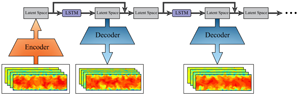
This study aims to build a PGDL model that can generate realistic turbulent datasets using a combination of the  ${\rm MSC}_{\rm {SP}}$-AE and the LSTM model. Figure 2 illustrates the PGDL model. After training the model, the ${\rm MSC}_{{\rm SP}}$-AE can learn to map the flow fields obtained from the DNS to the latent space and reconstruct the flow fields back to the original resolution. On the other hand, the LSTM model can learn to predict the temporal evolution of the low-dimensional data, i.e. the latent space by feeding back the output from the model to the input and recursively predicting the flow at future time steps. Finally, the output from the LSTM model is applied to the decoder of the ${\rm MSC}_{{\rm SP}}$-AE and the temporal evolution of the flow fields is predicted with the same spatial resolution of the ground truth data. In this study, the open-source library TensorFlow 2.4.0 (Abadi et al. Reference Abadi2016) is used for the implementation of the model. A sample Python code for the presented model is available on the following web page: https://fluids.pusan.ac.kr/fluids/65416/subview.dot.

Figure 2. Schematic of turbulent inflow generation using the proposed PGDL model.
4. Results and discussion
4.1. Instantaneous predictions and turbulence statistics
Primarily, we examine the general capability of the proposed PGDL model to predict the flow fields. Figures 3 and 4 show the predicted instantaneous velocity fields at  $Re_\tau =180$ and $550$, respectively. Here the values of $t^{+}$ in each figure correspond to training time $\text {steps} = 10\,010$, 10 100 and 11 000, respectively. It can be observed that the PGDL model can predict the instantaneous velocity fields at $Re_\tau =180$ with a commendable agreement with the DNS data, in terms of both the main flow structure and the fluctuations. Although the prediction of the flow fields at $Re_\tau =550$ shows fewer details about the fluctuations, it reveals a relatively good agreement with the DNS data.

Figure 3. Instantaneous velocity fields at  $Re_\tau =180$. (a) Streamwise velocity. (b) Wall-normal velocity. (c) Spanwise velocity.

Figure 4. Instantaneous velocity fields at  $Re_\tau =550$. (a) Streamwise velocity. (b) Wall-normal velocity. (c) Spanwise velocity.
Our primitive studies revealed that using only the pixel content as a loss function results in the flow fields suffering from a lack of fluctuation details in the outer region of the boundary layer. Furthermore, by using the auto-encoder without the subpixel convolution layer, the results showed less accurate flow fields as reported in § 4.3.
As shown in figures 5 and 6, the probability density function (p.d.f.) plots of the generated velocity components and pressure for both  $Re_\tau =180$ and $550$ reveal a commendable agreement with the results obtained from the DNS data, thus indicating the ability of the model to predict the instantaneous flow fields.

Figure 5. Probability density function plots of the velocity components and pressure at  $Re_\tau =180$.

Figure 6. Probability density function plots of the velocity components and pressure at  $Re_\tau =550$.
The capability of the model to generate velocity fields with accurate spatial distribution is examined using two-dimensional cross-correlation  $(R_{\alpha \alpha }({\Delta } y,{\Delta } z ))$ plots of the velocity components as shown in figures 7 and 8, where $\alpha$ represents the velocity component. It can be observed from the figures that the correlation plots are generally in good agreement with those obtained from the DNS data, indicating the ability of the PGDL model to generate instantaneous flow fields with an accurate spatial distribution for both Reynolds numbers.

Figure 7. Two-dimensional cross-correlation plots of the velocity components at  $Re_\tau =180$.

Figure 8. Two-dimensional cross-correlation plots of the velocity components at  $Re_\tau =550$.
To further validate the PGDL model, the statistics of 20 000 generated flow fields are compared to the turbulence statistics obtained from the DNS of the flow at  $Re_\tau =180$ and $550$ in figures 9 and 10, respectively. As shown in figure 9(a), the mean streamwise velocity profile of the generated data shows excellent agreement with the profile obtained from the DNS within all of the linear viscous sublayer, buffer layer and logarithmic region. The root-mean-square (r.m.s.) profiles of the velocity components ( $u_{rms}$, $\upsilon _{rms}$ and $w_{rms}$) are shown in figure 9(b). The comparison reveals good agreement with the results obtained from the DNS. The mean Reynolds shear stress $(-\overline {u'\upsilon '})$ profile shows excellent agreement over the entire range of the wall distance, as shown in figure 9(c). The r.m.s. profile of the streamwise vorticity $(\omega _{rms})$ is shown in figure 9(d). Although the profile of the generated data shows a good agreement with the profile from the DNS, this agreement is slightly different from those in the aforementioned figures. The turbulence statistics of the flow at $Re_\tau =550$ show similar accuracy to those of the flow at $Re_\tau =180$ as shown in figure 10. However, the $-\overline {u'\upsilon '}$ profile slightly deviates from the profile obtained from the DNS for the region where the maximum shear stress occurs. Furthermore, the $\omega _{rms}$ profile shows more deviation compared with the flow at $Re_\tau =180$.

Figure 9. Turbulence statistics of the flow at  $Re_\tau =180$. (a) Mean streamwise velocity profile. (b) The r.m.s. profiles of the velocity components. (c) Mean Reynolds shear stress profile. (d) R.m.s. profile of the streamwise vorticity.

Figure 10. Turbulence statistics of the flow at  $Re_\tau =550$. (a) Mean streamwise velocity profile. (b) The r.m.s. profiles of the velocity components. (c) Mean Reynolds shear stress profile. (d) The r.m.s. profile of the streamwise vorticity.
One of the most important factors for evaluating the turbulent inflow generator is the capability to produce a realistic spectral content for the flow fields; otherwise, the generated turbulence would be dissipated within a short distance from the inlet of the domain. Figures 11 and 12 show the spanwise energy spectra  $(E_{\alpha \alpha }(k_{z}))$ of the velocity components at three different wall distances for the flow at $Re_\tau =180$ and $550$, respectively. It can be observed from figure 11 that the spectra of the flow at $Re_\tau =180$ are generally in good agreement with the spectra obtained from the DNS. However, a slight deviation can be observed at high wavenumbers; we believe that this deviation would be corrected in the main simulation domain after a short distance from the inlet. Despite the higher friction Reynolds number, the spectra of the flow at $Re_\tau =550$ show a reasonable accuracy as shown in figure 12. It is worth mentioning here that the temporal correlation plots $(R_{\alpha \alpha }(t))$ of the generated flow exhibit a trend similar to that of the results reported by Kim & Lee (Reference Kim and Lee2020) and Fukami et al. (Reference Fukami, Nabae, Kawai and Fukagata2019) as they are free of spurious periodicity, as shown in figures 13 and 14. This is one of the advantages of using machine learning to generate turbulent inflow conditions over the aforementioned recycling method, which suffers from spurious periodicity due to the periodic boundary condition and the limited domain size. It is also worth noting that we have tested the model with time steps up to 60 000, and the results have shown that the model still can predict the instantaneous flow fields, and reproduce turbulent statistics and spectra with commendable accuracy.

Figure 11. Spanwise energy spectra of the velocity components at  $Re_\tau =550$.

Figure 12. Spanwise energy spectra of the velocity components at  $Re_\tau =550$.

Figure 13. Temporal correlation plots of the velocity components at  $Re_\tau =180$.

Figure 14. Temporal correlation plots of the velocity components at  $Re_\tau =550$.
4.2. Effect of loss terms in  $MSC_{SP}$-AE loss function

In order to select the optimum coefficient of each loss term, the model was first trained with just  $L_{pixel}$, and the magnitude of the loss after successful training was recorded. The training was repeated with the other loss terms individually and the magnitude of each of them was recorded. After that, in order to avoid any bias during the training process, the order of the loss term coefficient was set to a suitable value. Finally, the training was repeated multiple times using all the loss terms with variations in the values of the coefficients in every training to achieve the most stable training and optimum performance. As mentioned in § 3.1, each term in the loss function positively affects the output of the ${\rm MSC}_{{\rm SP}}$-AE. The effect of $L_{gradient}$ and $L_{perceptual}$ can be seen in figure 15. Here case 1 and case 2 represent the results from the ${\rm MSC}_{{\rm SP}}$-AE with and without using $L_{gradient}$ and $L_{perceptual}$, respectively. As can be observed from the figure, the blurry output from the ${\rm MSC}_{{\rm SP}}$-AE can be remarkably mitigated by using $L_{gradient}$ and $L_{perceptual}$. Figure 16 shows the effect of $L_{Reynolds\ stress}$. Here case 1 and case 2 represent the results from the ${\rm MSC}_{{\rm SP}}$-AE with and without using $L_{Reynolds\ stress}$, respectively. The impact of the Reynolds stress constraint on the turbulence statistics can be observed from the figure, especially for the region where the maximum shear stress occurs. As shown in figure 17, the spectra of the velocity components can be remarkably improved by using $L_{spectrum}$ (case 1) in the loss function compared with case 2, i.e. without using $L_{spectrum}$. These results indicate that the loss terms that are combined with $L_{pixel}$ can effectively improve the performance of the ${\rm MSC}_{{\rm SP}}$-AE.

Figure 15. Instantaneous velocity fields at  $Re_\tau =180$; case 1 and case 2 represent the results from the ${\rm MSC}_{{\rm SP}}$-AE with and without using $L_{gradient}$ and $L_{perceptual}$, respectively. (a) Streamwise velocity. (b) Wall-normal velocity. (c) Spanwise velocity.

Figure 16. The r.m.s. profiles of the velocity components (a) and mean Reynolds shear stress profile (b) at  $Re_\tau =180$; case 1 and case 2 represent the results from the ${\rm MSC}_{{\rm SP}}$-AE with and without using $L_{Reynolds\ stress}$, respectively.

Figure 17. Spanwise energy spectra of the velocity components at  $Re_\tau =180$; case 1 and case 2 represent the results from the ${\rm MSC}_{{\rm SP}}$-AE with and without using $L_{spectrum}$, respectively. Results at $y^{+}=5.4$.
4.3. Effect of subpixel convolution layer
The effect of the subpixel convolution layer on the  ${\rm MSC}_{{\rm SP}}$-AE performance is investigated in this section. Three cases are considered to examine the impact of the subpixel convolution layer: case 1, where the ${\rm MSC}_{{\rm SP}}$-AE is used; case 2, where two convolution layers are added after the last upsampling layer (which is used instead of the subpixel convolution layer) with 16 and 4 filters, respectively; and case 3, where two convolution layers each with four filters are added after the last upsampling layer. In both cases 2 and 3, the convolution layer before the last upsampling layer has 16 filters, whereas in case 1, the convolution layer before the subpixel convolution layer has just four filters. Figure 18 shows the reconstructed instantaneous velocity fields for all three cases. Here it can be seen clearly that case 1 shows more flow details with accurate values compared with case 2. Furthermore, it is obvious that the auto-encoder in case 3 failed to reconstruct realistic instantaneous velocity fields due to the few filters that extract features from the flow fields before the last convolution layer.

Figure 18. Instantaneous velocity fields at  $Re_\tau =180$; case 1, case 2 and case 3 represent the results from ${\rm MSC}_{{\rm SP}}$-AE, auto-encoder having convolution layer with 16 filters after the last upsampling layer and auto-encoder having convolution layer with four filters after the last upsampling layer, respectively. (a) Streamwise velocity. (b) Wall-normal velocity. (c) Spanwise velocity.
The root-mean-square error (RMSE) plots for the reconstructed velocity components and pressure using the auto-encoders in the three cases are plotted along the range of the wall distance in figure 19. Here it can be seen that the error shows higher values in case 2 compared with the error in case 1, and as expected, shows a rapid increase in the values in case 3. This indicates that the subpixel convolution layer outperformed the combination of the upsampling-convolution layers even with adding more filters to the convolution layers before and after the upsampling layer. Note that in case 2, the number of trainable parameters is more than the number of trainable parameters in case 1 due to the additional filters, and this results in a noticeable increase in the training time. Hence, the subpixel convolution layer which can remarkably improve the resolution of the flow fields can also help in reducing the training time of the auto-encoder.

Figure 19. Profiles of RMSE for the reconstructed velocity components and pressure at  $Re_\tau =180$; case 1, case 2 and case 3 represent the results from ${\rm MSC}_{{\rm SP}}$-AE, auto-encoder having convolution layer with 16 filters after the last upsampling layer and auto-encoder having convolution layer with four filters after the last upsampling layer, respectively. (a) Streamwise velocity. (b) Wall-normal velocity. (c) Spanwise velocity. (d) Pressure.
4.4. Effect of the number of LSTM branches
As shown in figure 1(b), a parallel stacked LSTM layers-based model is used in this study for modelling the temporal evolution of the latent space. Here the function of the parallelisation of the stacked LSTM layers is to decompose the latent space into different groups of features and model the temporal evolution of each group separately before obtaining the final output represented by the summation of all the branches passing through a dense layer. The optimum architecture of the LSTM model is selected based on the results obtained from using different numbers of branches of the LSTM model. Figure 20 shows the RMSE of the predicted latent space by the LSTM model using different numbers of branches. As can be observed from the figure, the error values decrease as the number of branches increases. Nevertheless, adding more branches results in an increase in the computational cost of the model, i.e. the training time. Furthermore, it can be observed that even with increasing the number of the LSTM branches to four, the RMSE value does not decrease significantly compared with the value when three branches are used. Note that the results obtained in this test are based on latent space of size = 512. Here the performance of the LSTM model is highly affected by the size of the latent space which also affects the reconstruction accuracy of the  ${\rm MSC}_{{\rm SP}}$-AE.

Figure 20. RMSE of the predicted latent space by the LSTM model using different numbers of LSTM branches;  $Re_\tau =180$.
4.5. Effect of latent space size
The size of the latent space in the  ${\rm MSC}_{{\rm SP}}$-AE is an important factor in designing the presented PGDL model, since changing the size of the latent space can affect both the ${\rm MSC}_{{\rm SP}}$-AE and the LSTM model performance. As mentioned in § 3.1, the size of the latent space is carefully selected to obtain the optimum latent space that can guarantee the reconstruction accuracy of the ${\rm MSC}_{{\rm SP}}$-AE and the ability of the LSTM model to predict the flow dynamics. Nakamura et al. (Reference Nakamura, Fukami, Hasegawa, Nabae and Fukagata2021) showed that using latent space with a very small size can make the auto-encoder fail to reconstruct the details of the flow fields which can result in inaccurate turbulence statistics. Here we test the PGDL model using three different latent space sizes, i.e. 128, 512 and 2048.
Figure 21 shows the RMSE plots for the velocity components and pressure predicted by the PGDL model along the range of the wall distance using the three latent space sizes. It is clearly shown that there is a noticeable difference between the error values for the cases of latent space  $\text {size} = 128$ and 512 due to the limited information on the flow fields when the latent space of $\text {size} = 128$ is used, while no significant difference can be seen between the latent space of $\text {size} = 512$ and 2048, indicating that the latent space with $\text {size} = 512$ is sufficient for representing the low-dimensional data in the ${\rm MSC}_{{\rm SP}}$-AE that can be modelled using the LSTM model.

Figure 21. Profiles of RMSE for the predicted velocity components and pressure at  $Re_\tau =180$; here 128, 512 and 2048 represent the sizes of the latent space. (a) Streamwise velocity. (b) Wall-normal velocity. (c) Spanwise velocity. (d) Pressure.
Furthermore, in order to examine the capability of the PGDL model with different latent space sizes to predict the dynamics of the flow, the largest Lyapunov exponent ( $\lambda _1$) is obtained from the predicted velocity data at different wall distances. The largest Lyapunov exponent can be calculated from the average rate of the exponential divergence between infinitely close trajectories in phase space. The positive Lyapunov exponent determines that the attractor has a chaotic behaviour. In this study, we use the method proposed by Rosenstein, Collins & De Luca (Reference Rosenstein, Collins and De Luca1993) to calculate $\lambda _1$, which is robust to changes in the embedding dimension, the size of the data and the reconstruction delay. Here the largest Lyapunov exponent can be calculated as a least-square fit to the line defined by
 \begin{equation} l(i)= \frac{1}{\Delta t}\langle \ln\,d_j(i) \rangle, \end{equation}
where  $d_j(i)$ is the distance of the $j$th pair of nearest neighbours, as a function of subsequent time steps. The angle brackets represent the averaging process over all the values of $j$.
$j$.
Figure 22 shows the plots of the average divergence rate of instantaneous velocity components at different wall distances using the three sizes of latent space. As shown in the figure, by using the smallest latent space, the plots show a noticeable deviation from the results obtained from the DNS data which results in noticeably different largest Lyapunov exponent values, whereas the plots obtained from the predicted velocity components using the latent spaces of size = 512 and 2048 show a similar trend with Lyapunov exponent values close to those obtained from the DNS data. These results indicate that the presented PGDL model with a latent space of size 512 can successfully model the dynamics of the flow parameters with commendable accuracy.

Figure 22. Plots of the average divergence rate of instantaneous velocity components at  $Re_\tau =180$ using the three sizes of latent space (128, 512 and 2048). (a) Streamwise velocity. (b) Wall-normal velocity. (c) Spanwise velocity.
5. Transfer learning and computational cost
The availability of the training data and the computational cost represented by the training time are crucial factors in deep-learning-based models. One of the approaches that can remarkably help in reducing the amount of training data and the time required for training is applying TL. Transfer learning is a technique that allows reusing the weights of a pretrained model for training another model rather than initialising the model with random values of the weights.
Guastoni et al. (Reference Guastoni, Güemes, Ianiro, Discetti, Schlatter, Azizpour and Vinuesa2021) reported the possibility of applying TL to a CNN-based model used to predict the flow fields of turbulent channel flow from wall quantities at  $Re_\tau = 180$ and 550. We recently (Yousif, Yu & Lim Reference Yousif, Yu and Lim2021) showed that TL can effectively help in decreasing the amount of the training data and training time by applying it to a GAN-based model used for reconstructing high-resolution velocity fields of turbulent channel flow at $Re_\tau = 180$ and 550 from extremely low-resolution data.
In this study, the TL approach is further extended to be applied to both the spatial mapping represented by the  ${\rm MSC}_{{\rm SP}}$-AE and the temporal mapping represented by the LSTM model by means of initialising the PGDL model of the flow at $Re_\tau =550$ with the weights obtained from training the model on data of the flow at $Re_\tau =180$.
Here the learning rate is reduced by a factor of 20 % to prevent the optimiser from rapidly diverging from the initialised weights. The RMSE for the PGDL model output using TL with different percentages of the full training data is plotted against the range of the wall distance in figure 23. It can be observed from the figure that by using just 25 % of the full training data with the aid of TL, the errors for the wall-normal velocity, spanwise velocity and pressure show values that are similar to those when the model is trained with the full data without TL for all of the wall distance range. Furthermore, when TL is used, the error for the streamwise velocity shows lower values for most of the wall distance range with a noticeable reduction in the values near the wall, regardless of the amount of training data. This indicates that TL can also improve the performance of the model, considering the transferred knowledge from the flow at  $Re_\tau = 180$.

Figure 23. Profiles of RMSE for the predicted velocity components and pressure at  $Re_\tau =550$ without and with TL using different percentages of the full training data. (a) Streamwise velocity. (b) Wall-normal velocity. (c) Spanwise velocity. (d) Pressure.
Finally, the computational cost of the proposed PGDL model should be noted. The total number of trainable parameters of the model is approximately 130 million (when a latent space of  $\text {size} = 512$ is used in the ${\rm MSC}_{{\rm SP}}$-AE and three LSTM branches are used in the LSTM model). The training of the ${\rm MSC}_{{\rm SP}}$-AE on a machine with a single NVIDIA TITAN RTX graphics processing unit (GPU) requires approximately 20 h, whereas the training of the LSTM model requires approximately 4 h. Hence, the total training time of the PGDL model is approximately 24 h.
The computational cost of the model can be remarkably decreased by utilising TL as reported in table 2. Here the time required for training the model is reduced by a factor of 80 % when 25 % of the full training data are used with TL. These results indicate that TL is an efficient approach that can be utilised to transfer the knowledge of turbulent flow at different Reynolds numbers, which can overcome the main drawback of deep learning, i.e. the amount of training data that are needed to obtain successful training and the time that is required for the training process.
Table 2. Number of trainable parameters and computational cost of the PGDL model.

6. Conclusions
This paper presented an efficient method for generating turbulent inflow conditions using an  ${\rm MSC}_{{\rm SP}}$-AE and an LSTM model. The physical constraints represented by the gradient of the flow, Reynolds stress tensor and spectral content were combined with the pixel information and the features extracted using VGG-19 to form the loss function of the ${\rm MSC}_{{\rm SP}}$-AE. The PGDL model was trained using DNS data extracted from a plane normal to the streamwise direction ( $y-z$ plane) of turbulent channel flow at $\textit {Re}_{\tau } = 180$ and 550. First, the ${\rm MSC}_{{\rm SP}}$-AE was trained to compress the high-dimensional instantaneous turbulence to a latent space and then reconstruct the flow fields with the same spatial resolution of the ground truth data. The LSTM model was subsequently trained to model the temporal evolution of the latent space. Finally, the predicted low-dimensional data were decoded using the decoder of the ${\rm MSC}_{{\rm SP}}$-AE to reconstruct the instantaneous flow fields. The proposed PGDL model accurately reconstructed the instantaneous flow fields and successfully reproduced the turbulence statistics with commendable accuracy for both $\textit {Re}_{\tau } = 180$ and 550. Furthermore, the spectra of the velocity components were favourably reproduced by the model, with a slight deviation from the spectra obtained from the DNS data at high wavenumbers for the flow at $\textit {Re}_{\tau } = 180$ and this deviation increased for the flow at $\textit {Re}_{\tau } = 550$.
The examination of each loss-term effect in the  ${\rm MSC}_{{\rm SP}}$-AE loss function revealed that each loss term can improve the performance of the ${\rm MSC}_{{\rm SP}}$-AE in a certain direction. The use of the subpixel convolution layer showed a remarkable improvement in the performance of the ${\rm MSC}_{{\rm SP}}$-AE in terms of the resolution of the flow fields compared with the use of the equivalent convolution and upsampling layers. The LSTM model performance was also investigated in terms of the effect of the number of branches. The results showed that a number of three branches can be optimum in terms of prediction accuracy and computational cost. The ability of the PGDL model to model the flow dynamics using different latent space sizes was examined through the RMSE of the predicted flow and Lyapunov exponent. Here the model was able to model the flow dynamics using a latent space of $\text {size} = 512$ with well-accepted precision.
Furthermore, the possibility of performing TL using different amounts of training data was examined by using the weights of the model trained on data of the flow at  $\textit {Re}_{\tau } = 180$ to initialise the weights for training the model with data of the flow at $\textit {Re}_{\tau } = 550$. The results revealed that by using only 25 % of the full training data, the time required for successful training can be reduced by a factor of approximately 80 % with a noticeable decrease in the RMSE values for the streamwise velocity component compared with the values when the full data were used without TL.
The results obtained from the present study suggest that the proposed model is efficient in terms of accuracy and computational cost. The present study showed that CNN has the capability to deal with the spatial mapping of turbulent flow fields; with the aid of a suitable physics-based loss function, CNN-based models can serve as an efficient data-driven method that can be utilised in the turbulence research area.
Funding
This work was supported by ‘Human Resources Program in Energy Technology’ of the Korea Institute of Energy Technology Evaluation and Planning (KETEP), granted financial resource from the Ministry of Trade, Industry & Energy, Republic of Korea (no. 20214000000140). In addition, this work was supported by the National Research Foundation of Korea (NRF) grant funded by the Korea government (MSIP) (no. 2019R1I1A3A01058576). This work was also supported by the National Supercomputing Center with supercomputing resources including technical support (KSC-2021-CRE-0244).
Declaration of interests
The authors report no conflict of interest.


 Open access