


1. Introduction
Settling of a drop through another immiscible fluid is a classical problem that has long captured the interest of the scientific and the engineering communities alike. Indeed, settling of drops remains relevant to a wide spectrum of natural and industrial processes such as oil recovery (Wasan et al. Reference Wasan, Shah, Aderangi, Chan and McNamara1978; Frising, Noïk & Dalmazzone Reference Frising, Noïk and Dalmazzone2006; Zhou et al. Reference Zhou, Yin, Chen, Liu and Zhang2019), food and cosmetics processing (Brummer Reference Brummer2006; Dickinson Reference Dickinson2011; Lamba, Sathish & Sabikhi Reference Lamba, Sathish and Sabikhi2015; Varvaresou & Iakovou Reference Varvaresou and Iakovou2015; Venkataramani, Tsulaia & Amin Reference Venkataramani, Tsulaia and Amin2020) as well as in the pharmaceutical industry, where droplets are used as the carriers and protectors of sensitive particles (Dams & Walker Reference Dams and Walker1987; Zhang, Chan & Leong Reference Zhang, Chan and Leong2013; Iqbal et al. Reference Iqbal, Zafar, Fessi and Elaissari2015). The first theoretical efforts to estimate the settling velocity of a drop dates back to the work of Hadamard (Reference Hadamard1911) and Rybczynski (Reference Rybczynski1911), who independently considered a pure spherical drop falling under its own weight in an otherwise stationary unbounded medium. A rich body of literature has since followed (Taylor & Acrivos Reference Taylor and Acrivos1964; Rushton & Davies Reference Rushton and Davies1973; Stone & Leal Reference Stone and Leal1990; de Blois et al. Reference de Blois, Reyssat, Michelin and Dauchot2019; Castonguay et al. Reference Castonguay, Kailasham, Wentworth, Meredith, Khair and Zarzar2023; Michelin Reference Michelin2023), where more physically realistic paradigms such as the presence of bounding walls (Brenner Reference Brenner1961; Wacholder & Weihs Reference Wacholder and Weihs1972; Pozrikidis Reference Pozrikidis1990; Desai & Michelin Reference Desai and Michelin2021; Jadhav & Ghosh Reference Jadhav and Ghosh2021a), alongside the impact of externally imposed fields (Barton & Subramanian Reference Barton and Subramanian1990; Das et al. Reference Das, Mandal, Som and Chakraborty2017; Das, Mandal & Chakraborty Reference Das, Mandal and Chakraborty2018; Poddar et al. Reference Poddar, Mandal, Bandopadhyay and Chakraborty2018, Reference Poddar, Mandal, Bandopadhyay and Chakraborty2019) have been accounted for both numerically (Pozrikidis Reference Pozrikidis1990; Stone & Leal Reference Stone and Leal1990; Li & Pozrikidis Reference Li and Pozrikidis1997; Tasoglu, Demirci & Muradoglu Reference Tasoglu, Demirci and Muradoglu2008) and analytically (Haber & Hetsroni Reference Haber and Hetsroni1971, Reference Haber and Hetsroni1972; Tsemakh, Lavrenteva & Nir Reference Tsemakh, Lavrenteva and Nir2004; Manor, Lavrenteva & Nir Reference Manor, Lavrenteva and Nir2008; Vlahovska, Bławzdziewicz & Loewenberg Reference Vlahovska, Bławzdziewicz and Loewenberg2009; Pak, Feng & Stone Reference Pak, Feng and Stone2014), towards computing the settling velocity of the drop.
It has long been established that multiphase systems such as those mentioned above inevitably contain surfactant-like impurities which either occur naturally or are added intentionally to stabilize such systems (Pal Reference Pal1992, Reference Pal2007; Zell et al. Reference Zell, Nowbahar, Mansard, Leal, Deshmukh, Mecca, Tucker and Squires2014). They tend to get adsorbed at the interface between the two phases and usually reduce the surface tension, which becomes a function of the local interfacial surfactant concentration. Hence, any fluid flow such as those generated by the settling of a drop, transport the surfactants, leading to a non-uniformity in their distribution, which in turn gives rise to surface tension gradients and thereby Marangoni stresses (Stone & Leal Reference Stone and Leal1990; Leal Reference Leal2007). Generally, the Marangoni stresses slow down the drops, the extent of which depends on the nature of the surfactants and the properties of the fluids (Levich & Krylov Reference Levich and Krylov1969; Holbrook & Levan Reference Holbrook and Levan1983a,Reference Holbrook and Levanb; Leal Reference Leal2007; Castonguay et al. Reference Castonguay, Kailasham, Wentworth, Meredith, Khair and Zarzar2023).
The exact manner in which surfactants influence the surface tension depends on the size of the surfactant molecules and the strength of the interactions between them, both of which may be mathematically described using specific adsorption isotherms. The simplest one among them is the ideal gas isotherm (Adamson & Gast Reference Adamson and Gast1967) which assumes the surfactant molecules to be point-like and non-interacting and the vast majority of the existing studies (Stone & Leal Reference Stone and Leal1990; Milliken, Stone & Leal Reference Milliken, Stone and Leal1993; Vlahovska, Loewenberg & Blawzdziewicz Reference Vlahovska, Loewenberg and Blawzdziewicz2005; Hanna & Vlahovska Reference Hanna and Vlahovska2010; Mandal, Ghosh & Chakraborty Reference Mandal, Ghosh and Chakraborty2016; Jadhav & Ghosh Reference Jadhav and Ghosh2021a) which investigate the influence of surface impurities on settling velocities use the ideal gas isotherm to model surfactant kinetics. Several others, such as Chen & Stebe (Reference Chen and Stebe1996) and Jadhav & Ghosh (Reference Jadhav and Ghosh2022), do consider the non-ideal aspects of the surfactants’ behaviour using the Frumkin and the van der Waals isotherms while probing the dynamics of drops and establish that factors such as surfactant packing play key roles in governing their settling velocity.
It is important to emphasize that most surfactants remain soluble in the bulk (from where adsorption–desorption takes place) to varying degrees, although the impact of their bulk solubility is routinely ignored in the literature while analysing their influence on droplet motion. Chen & Stebe (Reference Chen and Stebe1996) were among the first to account for adsorption–desorption from the bulk and showed that such interactions tend to remobilize the interface by making the surfactant distribution more uniform across it, thereby reducing the Marangoni stresses. Their analysis was performed in the kinetically limited regime, which requires the time scale of adsorption–desorption from the bulk to be much larger than the time scale of bulk diffusion close to the interface (Stebe & Barthes-Biesel Reference Stebe and Barthes-Biesel1995; Eggleton & Stebe Reference Eggleton and Stebe1998; Jin, Balasubramaniam & Stebe Reference Jin, Balasubramaniam and Stebe2004). This is of course an idealization since the bulk transport (advection and diffusion) of surfactants is naturally expected to alter the adsorption–desorption rates, the local surfactant concentrations as well as the remobilization of the interface (Muradoglu & Tryggvason Reference Muradoglu and Tryggvason2008; Sengupta, Walker & Khair Reference Sengupta, Walker and Khair2018; Lippera, Benzaquen & Michelin Reference Lippera, Benzaquen and Michelin2020a; Lippera et al. Reference Lippera, Morozov, Benzaquen and Michelin2020b; Morozov Reference Morozov2020; Chakraborty, Pramanik & Ghosh Reference Chakraborty, Pramanik and Ghosh2023). This issue, however, has hitherto remained poorly explored in the existing literature.
It is thus evident that there are still several open questions pertaining to the role played by surfactants in the settling of a drop that are yet to be properly addressed, despite this being a classical problem. First, although a bounding (or bottom) surface is omnipresent in any settling problem, its interactions with the surfactant kinetics remain largely unexplored, perhaps because of the analytical and even numerical challenges it poses owing to the continuously changing geometry. In a recent work, Jadhav & Ghosh (Reference Jadhav and Ghosh2021a) have shown that the impact of surface impurities on settling velocity may become more prominent close to the wall, although they only considered bulk-insoluble, ideal surfactants in the limit of diffusion-dominated interfacial transport. Second, the impact of the interactions between the bulk and the interfacial transport of surfactants on their kinetics, the overall motion of the drop and how these interactions evolve in the presence of a bounding wall have also remained an uncharted territory thus far.
To address some of the outstanding issues discussed above, in this article we analyse the settling dynamics of a drop towards a bounding wall in the presence of bulk-soluble, non-ideal surfactants which obey the Langmuir adsorption isotherm. The coupling between the bulk and the interfacial transport of surfactants is characterized by a bulk interaction parameter (Eggleton & Stebe Reference Eggleton and Stebe1998) ( $\omega$), defined in § 2.3. We subsequently construct a combined semi-analytical and numerical framework for arbitrary values of $\omega$, considering the bulk and the interfacial surfactant transport to be fully coupled. The special case of $\omega = 0$ associated with the kinetically limited regime (the decoupled limit) is also discussed as a reference case. The transports of surfactants are characterized by arbitrary interfacial and bulk Péclet numbers ( $Pe_s$ and $Pe_b$, respectively; see § 2.3) and hence are inherently unsteady in nature.
Our results confirm that the bulk solubility of surfactants indeed remobilizes a drop by acting as a source/sink for the surface impurities and its effects in doing so are the most prominent close to the wall. However, a finite rate of bulk diffusion of surfactants restricts the adsorption–desorption processes because of local depletion or accumulation of surfactants and therefore also hinders the remobilization of the drop. We further establish that an overall larger concentration of surfactants generally leads to stronger Marangoni stresses and thus results in a relatively slower motion of the drop.
The rest of the paper is arranged as follows. In § 2, we lay out the details of the physical system under consideration, the key assumptions, the important non-dimensional numbers along with the governing equations and boundary conditions. Section 3 discusses the details of the bispherical coordinate system, the arbitrary  $\omega$ framework for deducing the settling velocity (along with $\omega = 0$ scenario) and a brief outline of the semi-analytical-cum-numerical solution strategy. Section 4 presents the detailed results for the surfactant concentration distribution and droplet motion. Finally, we conclude in § 5.
2. The problem statement
2.1. Physical description of the system
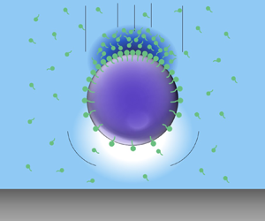
Figure 1 shows a schematic representation of the system under consideration. We consider the gravitational settling of a drop of radius  $a'$ towards a wall with velocity $\boldsymbol {U}'(t')$, which is a priori unknown. The outer fluid (fluid-1) has density $\rho '_1$ and viscosity $\mu '_1$, while the droplet (fluid-2) has density $\rho '_2$ ( $>\rho '_1$) and viscosity $\mu '_2$. Surfactant-like impurities are present in fluid-1 with uniform far-field bulk concentration $C'_{\infty }$ (< critical micelle concentration) and molecular diffusivity $D'_b$. These surfactant molecules get adsorbed onto the drop interface from the bulk. The interfacial surfactant concentration is $\varGamma '$ and its equilibrium value is denoted by $\varGamma '_{eq}$. The adsorption and desorption rate constants between the interface and the bulk are, respectively, taken as $k'_a$ and $k'_d$. The surface tension of a clean interface (with no surfactants) is $\gamma '_s$ and that with equilibrium surfactant concentration is $\gamma '_{eq} = \gamma '_{eq}(\varGamma '_{eq})$, where $\gamma '_{eq} < \gamma '_s$.

Figure 1. Schematic of a spherical drop of radius  $a'$ settling with velocity $\boldsymbol {U}' = -U'\hat {\boldsymbol {i}}_z$ due to its own weight towards a wall located at $z' = 0$. The continuous phase (fluid-1) and the droplet (fluid-2) have density $\rho '_1$ and $\rho '_2$ and viscosity $\mu '_1$ and $\mu '_2$, respectively. Dissolved surfactants are present in fluid-1 with far-field concentration $C'_{\infty } <$ critical micelle concentration, as well as at the droplet interface with equilibrium concentration $\varGamma '_{eq}$, governed by the adsorption from the bulk. The surface tension of the clean drop ( $\gamma '_s$) is reduced by the surfactants ( $\gamma '(\varGamma '_{eq})<\gamma '_s$). A bispherical coordinate system ( $\xi ',\eta ',\phi '$) is used in which the drop interface is located at $\xi ' = \alpha '(t')$. A reference cylindrical coordinate system ( $z',\rho ',\phi '$), with its origin on the wall ( $O$), is also shown.
A cylindrical coordinate system ( $z',\rho ',\phi '$) with origin at $O$ is defined such that the $z'$ axis passes through the droplet centre and the wall is located at $z' = 0$. An instantaneous bispherical coordinate system $(\xi ',\eta ',\phi ')$ allows us to define the wall at $\xi '=0$ together with the droplet surface at $\xi '=\alpha '(t')$, at any given instant. The instantaneous height of the droplet centre above the wall is denoted by $h'(t')$. Details of the bispherical coordinates can be found in § 3.1.
2.2. Key assumptions and the characteristic scales
For the rest of this article, we use dimensionless variables to describe any quantity. To this end, the non-dimensional version of any variable (say,  $A$) is chosen as $A = A'/A_c$, where $A_c$ is the characteristic scale for the said variable and the ‘prime’ symbol is dropped from the dimensional (with units) counterpart. Table 1 lists the characteristic scales chosen for all the pertinent variables herein.
Table 1. Characteristic scales chosen for the pertinent variables.

Before moving towards the formal analysis, it is important to point out some of the key assumptions made in this article. First, the flow is assumed to be viscosity-dominated and quasi-steady, on account of low Reynolds number ( $Re = \rho '_1 u_c a'/\mu '_1\ll 1$) and unit Strouhal number ( $St = t_c/(a'/u_c) = 1$). Second, we assume that the droplet deformation remains negligibly small throughout its motion on account of small capillary number ( $Ca = u_c \mu '_1/\gamma '_{eq}\ll 1$), generally true for creeping flows (Leal Reference Leal2007; Hanna & Vlahovska Reference Hanna and Vlahovska2010; Pak et al. Reference Pak, Feng and Stone2014) (see table 2). Third, it is assumed that the surfactant molecules undergo adsorption–desorption from the bulk obeying the Langmuir adsorption isotherm (Leal Reference Leal2007; Manikantan & Squires Reference Manikantan and Squires2020). As such, the molecules have a finite size and may only get adsorbed onto a finite number of lattice sites at the interface, although their intermolecular interactions are considered to be negligible. This limits the maximum possible surfactant concentration at the interface to a finite value denoted by $\varGamma '_{\infty }$ (m $^{-2}$). The variation in the surface tension also follows directly from the choice of the isotherm (Leal Reference Leal2007; Manikantan & Squires Reference Manikantan and Squires2020). Although the presence of surfactants may lead to excess interfacial rheological stresses (Agrawal & Wasan Reference Agrawal and Wasan1979; Schwalbe et al. Reference Schwalbe, Phelan, Vlahovska and Hudson2011; Elfring, Leal & Squires Reference Elfring, Leal and Squires2016; Manikantan & Squires Reference Manikantan and Squires2017; Dandekar & Ardekani Reference Dandekar and Ardekani2020), those effects are ignored in the present study.
Table 2. Important non-dimensional numbers and their range of values. The following values have been chosen for the various characteristic scales:  $u_c \sim \textit {O}(10^{-6})$– $\textit {O}(10^{-3})$ m s $^{-1}$; $a'\sim \textit {O}(10^{-6})$– $\textit {O}(10^{-3})$ m; $D'_b\sim D'_s\sim \textit {O}(10^{-10})\ {\rm m}^2\ {\rm s}^{-1}$; $\gamma '_{eq} \sim 10^{-2}\ {\rm N}\ {\rm m}^{-1}$; $\mu '_1\sim \textit {O}(10^{-3})$– $\textit {O}(10^{-1})\ {\rm Pa}\,{\rm s}$. Data taken from Ferri & Stebe (Reference Ferri and Stebe2000). Here $T$ is the absolute temperature and $R$ is the universal gas constant.

2.3. The non-dimensional numbers
Upon enforcing the non-dimensionalization scheme mentioned above in the governing equations and the boundary conditions (the dimensional equations have been omitted for brevity) for fluid flow and surfactant transport, several key non-dimensional numbers emerge that dictate the physics of the problem. These non-dimensional numbers along with their expressions and the possible range of values are listed in table 2.
Of particular interest to us are the following entries: (i) the bulk and the surface Péclet numbers ( $Pe_b$ and $Pe_s$), which represent the ratio of the advective and the diffusive fluxes in the bulk and the interface, respectively; (ii) the Biot number ( $Bi$), which represents the ratio of the desorptive flux to the interfacial advective flux of the surfactants; (iii) the surfactant packing factor ( $\zeta$) and the adsorption number ( $K$) which are related to each other as $\zeta = KC_{s,eq}/(1+KC_{s,eq})$, where $C_{s,eq}$ is the bulk concentration next to the interface at equilibrium, $K$ represents the ratio of the adsorptive and the desorptive fluxes from the bulk and $\zeta$ quantifies the ratio of the equilibrium surfactant concentration to the maximum possible concentration on the interface; (iv) the adsorption depth ( $\delta$) which indicates the thickness of the depleted region near the interface because of adsorption (Eggleton & Stebe Reference Eggleton and Stebe1998); and (v) the bulk interaction parameter ( $\omega$), which itself is a composite number and represents the strength of coupling between the bulk and the interfacial transport.
Evidently,  $\zeta \rightarrow 1$ represents a very densely packed interface, while $\zeta \ll 1$ represents the ideal gas limit on account of dilute surfactant concentration. It is also important to note that although $Re \ll 1$, $Pe_b$ and $Pe_s$ may still be $O(1)$ or larger because molecular diffusivity of surfactants ( $D'$) is usually significantly smaller than the kinematic viscosities of various liquids. On the other hand, the insoluble surfactant limit (Leal Reference Leal2007) may be recovered by enforcing $Bi = 0$. Readers are referred to the work of Manikantan & Squires (Reference Manikantan and Squires2020) and Eggleton & Stebe (Reference Eggleton and Stebe1998) for further insights into the various numbers appearing in table 2. Detailed discussion of the significance of $\omega$ is postponed until § 3.2.
Figure 2 schematically depicts the physical mechanisms that various non-dimensional numbers mentioned above represent. Figure 2(a) illustrates bulk and interfacial advection, adsorption–desorption and accumulation of surfactants at the north pole of the drop due to its downward motion. Figure 2(b) exhibits a section of the interface with non-uniform surfactant concentration leading to Marangoni stresses (quantified by  $Ma$) and the adsorption depth around the interface where the bulk surfactant concentration is diluted as compared with its far-field value, because of adsorption onto the interface.

Figure 2. Schematic showing the role played by the various non-dimensional numbers listed in table 2. (a) The bulk Péclet number ( $Pe_b$), the surface Péclet number ( $Pe_s$) and the Biot number ( $Bi$) respectively contribute to the bulk and interfacial transport and the adsorption–desorption process. (b) The Marangoni number ( $Ma$) is associated with the surface tension gradient and adsorption depth ( $\delta$) is related to the rate of adsorption from the bulk.
2.4. The non-dimensional governing equations and boundary conditions
The interfacial surfactant concentration ( $\varGamma$) is governed by the following conservation equation (Wong, Rumschitzki & Maldarelli Reference Wong, Rumschitzki and Maldarelli1996; Eggleton & Stebe Reference Eggleton and Stebe1998; Leal Reference Leal2007):
 \begin{align} \left.\frac{\partial \varGamma}{\partial t}\right\rvert_{\xi,\eta} - \dot{\boldsymbol{\chi}} \boldsymbol{\cdot} \boldsymbol{\nabla}_s \varGamma + \boldsymbol{\nabla}_s\boldsymbol{\cdot}(\varGamma \boldsymbol{u}) =\frac{1}{Pe_s}\boldsymbol{\nabla}_s\boldsymbol{\cdot}(D_{s,{eff}} \boldsymbol{\nabla}_s \varGamma) + Bi\left[K C_s \left(\frac{1}{\zeta} -\varGamma\right)-\varGamma\right],\end{align}
where  $\boldsymbol {u}$ is the fluid velocity at the interface and $\boldsymbol {\nabla }_s = \boldsymbol {I}_s\boldsymbol {\cdot }\boldsymbol {\nabla }$ is the surface gradient operator, where $\boldsymbol {I}_s = (\boldsymbol {I}-\hat {\boldsymbol {n}}\hat {\boldsymbol {n}})$, $\boldsymbol {I}$ is the identity tensor and $\hat {\boldsymbol {n}}$ is the outward unit normal to the droplet interface. The transient term $\partial \varGamma /\partial t$ is evaluated at fixed surface coordinates ( $(\xi,\eta )$; defined later) (Wong et al. Reference Wong, Rumschitzki and Maldarelli1996). However, since the left-hand side of (2.1) is to be evaluated at a material point, a correction term, namely $\dot {\boldsymbol {\chi }}$, must be added (Wong et al. Reference Wong, Rumschitzki and Maldarelli1996) to account for the velocity of the coordinate system itself. Term $\dot {\boldsymbol {\chi }}$ represents the velocity of a point with fixed coordinates and its expression is provided in Appendix A. For non-deforming drops in Cartesian or spherical coordinate systems, $\dot {\boldsymbol {\chi }} = 0$; however, since we have chosen a bispherical coordinate in this work, generally $\dot {\boldsymbol {\chi }} \neq 0$ (see (A1)). Parameter $D_{s,{eff}}$ represents the effective surface diffusivity, whose expression may be derived using the Gibbs relation and for the Langmuir isotherm it reads $D_{s,{eff}} = (1-\zeta \varGamma )^{-1}$; see the work of Jadhav & Ghosh (Reference Jadhav and Ghosh2022) for further details. The last term on the right-hand side of (2.1) is the net adsorption flux onto the interface according to the Langmuir isotherm (Chen & Stebe Reference Chen and Stebe1996; Manikantan & Squires Reference Manikantan and Squires2020). A relation between $\zeta$ and $C_{s,eq}$ may be established based on the equilibrium configuration ( $\varGamma = 1$) when there is no net adsorption–desorption, and this leads to (Eggleton & Stebe Reference Eggleton and Stebe1998) $\zeta = K(1+K)^{-1}$ at equilibrium (with $C_{s,eq} = 1$). We emphasize that the interfacial transport at $Pe_s \geq O(1)$ is inherently unsteady in the present scenario because of the continuously changing geometry, although the flow itself is quasi-steady.
The bulk transport of surfactants in fluid-1 is governed by the advection–diffusion equation, given by (Eggleton & Stebe Reference Eggleton and Stebe1998; Lippera et al. Reference Lippera, Morozov, Benzaquen and Michelin2020b)
 \begin{equation} \left.\frac{\partial C}{\partial t}\right\rvert_{\xi,\eta} + (\boldsymbol{u}_1-\dot{\boldsymbol{\chi}})\boldsymbol{\cdot}\boldsymbol{\nabla} C = \frac{1}{Pe_b}\nabla^{2}C,\end{equation}
where  $C$ is the bulk concentration. We again note that similar to (2.1), the bulk transport is also inherently unsteady when $Pe_b \geq O(1)$. Therefore, akin to (2.1), for evaluating the time derivative $\partial C/\partial t$ at fixed coordinates ( $\xi, \eta$; defined later), a correction term needs to be added on the left-hand side to account for the velocity of the coordinate system. Equation (2.2) is subject to the far-field condition, $\boldsymbol {\nabla } C \rightarrow \boldsymbol {0}$ as $(\rho ^2 + z^2)^{1/2}\rightarrow \infty$, and no flux condition at the wall, $\hat {\boldsymbol {i}}_z\boldsymbol {\cdot } \boldsymbol {\nabla } C = 0$ at $z = 0$. At the droplet interface, the bulk diffusion flux balances the net adsorption–desorption flux, which may be expressed as (Manikantan & Squires Reference Manikantan and Squires2020)
 \begin{equation} \hat{\boldsymbol{n}} \boldsymbol{\cdot} \boldsymbol{\nabla} C = \omega \left[K C_s \left(\frac{1}{\zeta} -\varGamma\right)-\varGamma\right] = \omega[C_s(1+K(1-\varGamma)) - \varGamma].\end{equation}
According to (2.3), the bulk interaction parameter ( $\omega = Bi Pe_b \delta$) may also be interpreted as the ratio of the adsorption–desorption flux to the diffusive flux of the surfactant at the interface. It is evident that the above condition couples the bulk and the interfacial transport processes ((2.2) and (2.1)), the strength of which is determined by $\omega$.
The flow in the  $i$th fluid (for $i = 1, 2$) satisfies
 \begin{equation} \nabla^2\boldsymbol{u}_i = \boldsymbol{\nabla} p_i, \quad \boldsymbol{\nabla}\boldsymbol{\cdot}\boldsymbol{u}_i = 0,\end{equation}
subject to far-field condition  $\boldsymbol {u}_1\rightarrow 0$ as $(\rho ^2 + z^2)^{1/2}\rightarrow \infty$ and the boundedness condition is $|\boldsymbol {u}_2|<\infty, |p_2|<\infty$, inside the drop. At the wall, no-slip and no-penetration conditions imply $\boldsymbol {u}_1\boldsymbol {\cdot }\hat {\boldsymbol {i}}_{\rho } = 0, \boldsymbol {u}_1\boldsymbol {\cdot }\hat {\boldsymbol {i}}_z = 0$, at $z = 0$. The boundary conditions at the (non-deforming) droplet interface take the following form (Leal Reference Leal2007):
 $$\begin{gather} \hat{\boldsymbol{u}}_1\boldsymbol{\cdot} \hat{\boldsymbol{n}} = \hat{\boldsymbol{u}}_2\boldsymbol{\cdot} \hat{\boldsymbol{n}} = 0, \end{gather}$$
 $$\begin{gather}\boldsymbol{I}_s\boldsymbol{\cdot} \hat{\boldsymbol{u}}_1 = \boldsymbol{I}_s\boldsymbol{\cdot}\hat{\boldsymbol{u}}_2, \end{gather}$$
 $$\begin{gather}\boldsymbol{I}_s\boldsymbol{\cdot}\left[(\boldsymbol{\tau}_1 - \lambda\boldsymbol{\tau}_2) \boldsymbol{\cdot} \hat{\boldsymbol{n}} + \frac{\boldsymbol{\nabla}_s \gamma(\varGamma)}{Ca}\right]= 0. \end{gather}$$
In the above, (2.5a) and (2.5b) are, respectively, the no-slip and the velocity continuity conditions. Equation (2.5c) expresses the tangential stress balance, where  $\boldsymbol {\tau }_i$ is the viscous stress in the $i$th fluid ( $i = 1,2$), defined as $\boldsymbol {\tau }_i = \boldsymbol {\nabla }\boldsymbol {u}_i + (\boldsymbol {\nabla }\boldsymbol {u}_i)^T$, and $\lambda = \mu '_2/\mu '_1$ is the viscosity ratio. The Marangoni stress is represented by $\boldsymbol {\nabla }_s \gamma /Ca$, where the surface tension, $\gamma (\varGamma )$, can be written as follows, based on the Langmuir isotherm (Eggleton & Stebe Reference Eggleton and Stebe1998):
 \begin{equation} \gamma = 1 + Ma Ca \ln\left(\frac{1-\zeta\varGamma}{1-\zeta}\right).\end{equation}
3. Analysis of droplet motion
3.1. The bispherical coordinate system
The (spherical) droplet interface and the wall may be simultaneously represented as coordinate surfaces using the bispherical coordinate system ( $\xi,\eta,\phi$), where $\xi$ represents a set of non-intersecting spheres and $\eta$ ( $0\leq \eta \leq {\rm \pi}$) represents the position on a particular sphere. The origin ( $O$) coincides with the cylindrical coordinate system as depicted in figure 1. It is to be noted that at every time instant a new bispherical coordinate has to be defined, since the droplet continuously falls towards the wall. We follow the convention used by Lippera et al. (Reference Lippera, Morozov, Benzaquen and Michelin2020b), who analysed the axisymmetric motion of an active drop towards a rigid wall. At any instant $t$, the relation between a point in the fixed cylindrical coordinate system ( $z,\rho,\phi$) and the bispherical coordinate system ( $\xi,\eta,\phi$) is given by (Happel & Brenner Reference Happel and Brenner1983; Lippera et al. Reference Lippera, Morozov, Benzaquen and Michelin2020b)
 \begin{equation} \rho = \frac{c_0(t)\sqrt{1-\nu^2}}{\mathcal{L}}, \quad z = \frac{c_0(t)\sinh{(\alpha(t)\xi)}}{\mathcal{L}},\end{equation}
where  $\mathcal {L}(\xi,\nu,t) = \cosh {(\alpha (t)\xi )} - \nu$ and $\nu = \cos {\eta }$. The parameter $\alpha$ depends upon the distance of the centre of the drop from the wall ( $h(t)$) as $\alpha (t) = \cosh ^{-1}{(h(t))}$, and $c_0$ is a positive constant defined as $c_0(t) = \sinh {\alpha (t)}$. As per the coordinate system defined in (3.1a,b), at any instant the drop surface and the wall are, respectively, denoted by $\xi = 1$ and $\xi = 0$. For a non-deforming spherical drop, the outward surface normal becomes $\hat {\boldsymbol {n}} = -\hat {\boldsymbol {i}}_{\xi }$ (see figure 1). The metric coefficients for bispherical coordinates are (Happel & Brenner Reference Happel and Brenner1983) $\ell _1 = \ell _2 = \mathcal {L}/c_0, \ell _3 = \mathcal {L}/(c_0\sqrt {1-\nu ^2})$, and the gradient operator is defined as $\boldsymbol {\nabla } = \hat {\boldsymbol {i}}_{\xi } \ell _1 \partial /\partial (\alpha \xi ) + \hat {\boldsymbol {i}}_{\eta } \ell _2 \partial /\partial \eta + \hat {\boldsymbol {i}}_{\phi } \ell _3 \partial /\partial \phi$.
It is straightforward to rewrite equations (2.1), (2.2) and (2.4a,b), along with the boundary conditions (2.3) and (2.5) in bispherical coordinates.
3.2. A closer look at the bulk interaction parameter ( $\omega$)

The bulk interaction parameter ( $\omega$) in (2.3) may be written as the ratio of two time scales: $\omega = t_{diff}^{GM}/t_{des}$, where $t_{des} \sim k'^{-1}_d$ is the time scale of desorption and $t_{diff}^{GM} \sim \delta ' a'/D'_b$ is the mean bulk diffusion time scale, which is the geometric mean of two distinct diffusion time scales (Jin et al. Reference Jin, Balasubramaniam and Stebe2004): $t_{diff}^{GM} = \sqrt {t_{diff}^{drop} t_{diff}^{ads}}$. The first of these ( $t_{diff}^{drop}$) is defined at the length scale of the drop itself, denoted as $t_{diff}^{drop} \sim a'^2/D'_b$, and the second is associated with the length scale of the adsorption layer, given by $t_{diff}^{ads} \sim \delta '^2/D'_b$. Therefore, $\omega \ll 1$ when $t_{diff}^{GM} \ll t_{des}$, implying that bulk diffusion is significantly faster in replenishing the bulk surfactant concentration as compared with desorption, resulting in a kinetically limited coupling between the bulk and the interfacial surfactant transport. The scenario corresponding to $\omega = 0$ represents the so-called ‘decoupled limit’, where the bulk diffusion is infinitely fast compared with the adsorption–desorption kinetics, and was the paradigm investigated by Chen & Stebe (Reference Chen and Stebe1996). On the other hand, $\omega \sim O(1)$ implies that bulk diffusion and interfacial adsorption–desorption occur at about the same rate, which may lead to significant variations in the bulk surfactant concentrations around the drop, as we show later. The key role played by the geometric mean of two distinct diffusion times scales is not very dissimilar to what is observed in the case of charging–discharging of electrical double layers where the resistance–capacitance time scale ( $t_{RC}$) becomes important (Kilic, Bazant & Ajdari Reference Kilic, Bazant and Ajdari2007). Akin to $t_{diff}^{GM}$, $t_{RC}$ is also the geometric mean of two diffusion times scales, one associated with the overall geometry and a second associated with diffusion across the electrical double layer.
Table 2 shows that it is possible to write  $\omega = BiPe_b\delta$. The Biot number may be expressed as the ratio of advection and desorption time scales: $Bi \sim t_{adv}/t_{des}$, where $t_{adv} \sim a'/u_c$. Therefore, for small $Bi$, the desorption rate becomes very slow ( $t_{des} \gg 1$), resulting in a small value of $\omega$. Similarly, the bulk Péclet number may be expressed as the ratio of the bulk diffusion time scale (at the length scale of the drop) and the advective time scale: $Pe_b \sim t_{diff}^{drop}/t_{adv}$. Hence, $Pe_b \to 0$ entails very fast bulk diffusion ( $t_{diff}^{drop} \to 0$), resulting in $\omega \to 0$, even when $Bi \neq 0$. Finally, recall that the adsorption depth is defined as $\delta = \varGamma '_{eq}/(C'_{\infty }a')$. Therefore, $\delta \to 0$ refers to an infinitely large bulk concentration ( $C'_{\infty } \rightarrow \infty$), such that any change in concentration because of adsorption–desorption near the interface is instantaneously replenished by very fast local diffusion (i.e. $t_{diff}^{ads} \sim \delta '^2/D'_b \to 0$). This will also result in $\omega \to 0$, without explicitly requiring $Bi \to 0$.
In what follows, we seek to construct a combined semi-analytical and numerical framework to solve the equations in § 2.4 for a finite speed of bulk diffusion (i.e. arbitrary  $\omega$). The decoupled limit ( $\omega = 0$) is taken as the reference case. At the same time, we also consider $Bi$,
$Bi$,  $Pe_s$ and $Pe_b$ to remain $O(1)$ throughout the remainder of this article (which also entails $\omega \sim O(1)$ or larger). Table 2 exhibits that it is plausible for all of the above parameters to assume $O(1)$ values. We reiterate that in this article, the drop is assumed to be spherical (on account of $Ca \ll 1$) and, therefore, $O(Ca)$ corrections to the flow field are not considered.
3.3. General framework for arbitrary values of $\omega$

3.3.1. The flow field
The flow is axisymmetric and hence (2.4a,b) may be solved using the Stokes stream function ( $\varPsi$). In the bispherical coordinates, the velocity components in the $i$th fluid ( $\boldsymbol {u} = u_{\xi }\hat {\boldsymbol {i}}_{\xi } + u_{\eta }\hat {\boldsymbol {i}}_{\eta }$) are related to the stream function $\varPsi _i$ as (Mandal et al. Reference Mandal, Ghosh and Chakraborty2016; Lippera et al. Reference Lippera, Morozov, Benzaquen and Michelin2020b)
 \begin{equation} u_{\xi,i} ={-}\frac{\mathcal{L}^2}{c_0^2}\frac{\partial \varPsi_i}{\partial \nu}, \quad u_{\eta,i} ={-}\frac{\mathcal{L}^2}{\alpha c_0^2 \sqrt{1-\nu^2}}\frac{\partial \varPsi_i}{\partial \xi}. \end{equation}
Equation (2.4a,b) may then be expressed for the  $i$th fluid (Happel & Brenner Reference Happel and Brenner1983) as $\mathcal {E}^2 (\mathcal {E}^2 \varPsi _i) = 0$, where $\mathcal {E}^2= \partial ^2/\partial z^2 + \rho (\partial /\partial \rho )[\rho ^{-1}(\partial /\partial \rho )]$ (Brenner Reference Brenner1961). The general solution for $\varPsi$ in the bispherical coordinates is as follows (Stimson & Jeffery Reference Stimson and Jeffery1926; Lippera et al. Reference Lippera, Morozov, Benzaquen and Michelin2020b):
 \begin{equation} \varPsi_i(\xi,\nu,t) = \mathcal{L}^{{-}3/2}\sum_{n=1}^{\infty}n(n+1) \mathcal{W}_{n,i}(\xi,t) \mathcal{C}_{n+1}^{{-}1/2}(\nu),\end{equation}
where  $\mathcal {C}_{n+1}^{-1/2}(\nu )$ is the Gegenbauer polynomial of order $n+1$ and degree $-1/2$, and the functions $\mathcal {W}_{n,1}$ and $\mathcal {W}_{n,2}$ for, respectively, the outer and the inner fluids have the following form:
 \begin{align} \mathcal{W}_{n,1}(\xi,t) &= A_n(t)\cosh{\left[\left(n+\frac{3}{2}\right)\alpha\xi\right]} + B_n(t)\sinh{\left[\left(n+\frac{3}{2}\right)\alpha\xi\right]} \nonumber\\ &\quad + C_n(t)\cosh{\left[\left(n-\frac{1}{2}\right)\alpha\xi\right]} + D_n(t)\sinh{\left[\left(n-\frac{1}{2}\right)\alpha\xi\right]}, \end{align}
 \begin{align} \mathcal{W}_{n,2}(\xi,t) &= E_n(t)\, {\rm e}^{-(n+3/2)\alpha\xi} + F_n(t)\, {\rm e}^{-(n-1/2)\alpha\xi}, \end{align}
where the coefficients  $A_n$ to $F_n$ are to be evaluated at each time instant $t$. Based on (2.5), the boundary conditions for the velocity components at the droplet interface ( $\xi = 1$) become $u_{\xi,1} = u_{\xi,2} = -U \hat {\boldsymbol {i}}_z\boldsymbol {\cdot }\hat {\boldsymbol {i}}_{\xi }$ and $u_{\eta,1} = u_{\eta,2}$, while the stress balance condition takes the following form:
 \begin{equation} \tau_{\xi\eta,1} -\lambda\tau_{\xi\eta,2} - \frac{\zeta Ma(\cosh{\alpha}-\nu)\sqrt{1-\nu^2}}{c_0(1-\zeta\varGamma)}\frac{\partial \varGamma}{\partial \nu}= 0,\end{equation}
where  $U$ is the droplet velocity (yet unknown) and $\tau _{\xi \eta }$ is the tangential component of the viscous stresses, and its expression in bispherical coordinates is given in Appendix A. The rest of the boundary conditions remain unchanged. As such, the boundary conditions at the wall are $u_{\xi,1} = u_{\eta,1} = 0$ at $\xi = 0$.
It is important to note that the coefficients  $A_n$ to $F_n$ will be linear functions of $U$, provided $\varGamma$ is known in (3.5) – see the solution strategy discussed in § S1 in the supplementary material available at https://doi.org/10.1017/jfm.2024.406, along with (B8a,b) and the discussion before it in Appendix B.1. For instance, $A_n(t)$ may be expressed as $A_n(t) = \mathcal {U}_{1,1}(t;n) + U \mathcal {U}_{1,2}(t;n)$; the remaining coefficients may also be written in a similar form and their expressions are provided in Appendix B.1. The above boundary conditions may be used to determine a set of algebraic equations governing the coefficients $A_n$ to $F_n$ (or, equivalently, $\mathcal {U}_{1,1}, \mathcal {U}_{1,2},\ldots\,$, etc.) and these equations are included in Appendix B.1 (see (B3) therein). For computing the solutions for the coefficients, we have truncated the series in (3.3) after $N_1$ terms (see § 3.5 for further details).
3.3.2. The droplet velocity $(U)$ and position $(h)$


The droplet velocity is computed by carrying out an overall force balance. For quasi-steady flow, the hydrodynamic drag force ( $F'_D$) on the drop is balanced by the net gravitational force ( $F'_G =$ gravity-buoyancy) at every instant. The drag force may be expressed as (Mandal et al. Reference Mandal, Ghosh and Chakraborty2016; Jadhav & Ghosh Reference Jadhav and Ghosh2021a) $F'_D = 2\sqrt {2} \mu '_1 a' u_c {\rm \pi}\sum _{n=1}^{\infty } (A_n + B_n + C_n + D_n) n(n+1)/c_0$. The net gravitational force on the drop reads $F'_G = 4{\rm \pi} a'^3g'(\rho '_2-\rho '_1)/3$, where $g'$ is acceleration due to gravity. Now, using the definition for $u_c$ from table 1, the overall force balance takes the form
 \begin{equation} \sum_{n=1}^{\infty} (A_n + B_n + C_n + D_n) n(n+1) = \sqrt{2} c_0. \end{equation}
Upon using the appropriate form of the coefficients  $A_n$– $F_n$ as given in § 3.3.1 and Appendix B.1 in the above, and subsequently truncating the summation after $N_1$ terms, the droplet velocity $(U)$ may be computed.
The droplet position ( $h(t)$) is then governed by the following equation: ${\rm d}h/{\rm d}t = -U(h(t))$, which has to be solved at every time instant. However, (3.5) suggests that the surfactant concentration ( $\varGamma$) will also appear in these equations and hence must be determined, as discussed in the following.
3.3.3. The interface surfactant concentration $(\varGamma )$

The surfactant concentration on the droplet interface ( $\xi =1$) may be written as (Morozov Reference Morozov2020)
 \begin{equation} \varGamma(\nu,t) = \sum_{n=0}^{\infty} a_n(t) \mathcal{P}_n(\nu),\end{equation}
where  $\mathcal {P}_n(\nu )$ is the Legendre polynomial of order $n$ and degree $1$ and the coefficients $\boldsymbol {a}(t) = [a_0(t), a_1(t),\ldots ]$ are to be evaluated at each time instant $t$. Substituting (3.7) along with the expressions for the velocity field from (3.2a,b) and the surface divergence and gradient operators from Appendix A into (2.1) and subsequently using the identities for the Gegenbauer (see (B2)) and the Legendre (see (B10a,b)) polynomials, the same may be transformed into a system of ordinary differential equations (ODEs) provided in Appendix B.2 (see (B11) therein).
Upon using the orthogonality property of the Legendre polynomials, a set of ODEs for the individual coefficients  $a_{r}$ ( $r=0, 1, 2, \ldots$) may be determined from (B11) as follows:
 \begin{equation} \frac{{\rm d} a_r}{{\rm d}t} = \frac{1}{2}(2r+1) \mathcal{B}_r(\nu,t,\boldsymbol{a}).\end{equation}
The functional form of  $\mathcal {B}_r$ is provided in (B14). The above set of ODEs have been solved using a fourth-order Runge–Kutta method by truncating the series in (3.7) after $N_2$ terms (see § 3.5 for further details).
3.3.4. The bulk surfactant concentration $(C)$

Taking hint from the general solution for the Laplace equation in bispherical coordinates (Jeffery Reference Jeffery1912) (see (C1) in Appendix C), we have chosen  $C$ to be of the following form, such that its variations vanish at infinity (Lippera et al. Reference Lippera, Morozov, Benzaquen and Michelin2020b):
 \begin{equation} C(\xi,\nu,t) = 1+ \mathcal{L}^{1/2}\sum_{n=0}^{\infty} b_n(\xi,t) \mathcal{P}_n(\nu), \end{equation}
where the functions  $b_n(\xi,t)$ are to be determined. Upon substituting (3.9) into (2.2) and using the identities for the Legendre polynomials (see (B10a,b)), (2.2) may be transformed into a system of partial differential equations, reported as (B15) in Appendix B.3. Then an equation governing the $r$th mode (i.e. $b_r, r = 0, 1, 2, \ldots$) may be extracted from (B15) using the orthogonality condition for the Legendre polynomials as follows:
 \begin{equation} \frac{2}{2r+1}\frac{\partial b_r}{\partial t} + \sum_{k=0}^{\infty} \left[\frac{\partial^2 b_k}{\partial \xi^2} \mathcal{H}_{kr}(\xi,t) + \frac{\partial b_k}{\partial \xi} \mathcal{G}_{kr}(\xi,t) + b_k \mathcal{D}_{kr}(\xi,t) \right]= 0.\end{equation}
The expressions for the entities  $\mathcal {H}_{kr}$, $\mathcal {G}_{kr}$ and $\mathcal {D}_{kr}$ are provided in Appendix B.3 (see (B17) therein). Similarly, the boundary conditions for $C$ stated earlier (after (2.2)) may be recast using (3.9) as
 $$\begin{gather} \sum_{k=0}^{\infty}\left.\left((\cosh{(\alpha\xi)} \mathcal{R}^0_{kr} - \mathcal{R}^1_{kr})\frac{\partial b_k}{\partial \xi} + \left(\frac{\alpha \sinh{(\alpha\xi)}}{2} \mathcal{R}^0_{kr} + \mathcal{V}_{kr}\right)b_k\right)\right\rvert_{\xi = 1} = \mathcal{Q}_r\rvert_{\xi = 1}, \end{gather}$$
 $$\begin{gather}\left.\left(\frac{\partial b_r}{\partial \xi} - \frac{r+1}{2r+3}\frac{\partial b_{r+1}}{\partial \xi} - \frac{r}{2r-1}\frac{\partial b_{r-1}}{\partial \xi} \right)\right\rvert_{\xi = 0} = 0, \end{gather}$$
wherein the expressions for  $\mathcal {R}^0_{kr},\mathcal {R}^1_{kr},\mathcal {V}_{kr}$ and $\mathcal {Q}_r$ are included in Appendix B.3. Equations (3.10) subject to (3.11) have been solved using an implicit finite difference scheme, by truncating the series in (3.9) (and consequently (3.10) and (3.11a)) after $N_3$ terms (see § 3.5 for further details).
3.4. The decoupled limit $(\omega = 0)$

In the decoupled limit, the bulk surfactant concentration ( $C$) satisfies an equation of the form (2.2), subject to the initial condition $C = 1$ everywhere, the far-field condition $\boldsymbol {\nabla } C\rightarrow \boldsymbol {0}$ and the no-flux condition at the wall $\hat {\boldsymbol {i}}_z\boldsymbol {\cdot } \boldsymbol {\nabla } C = 0$ (at $z = 0$), while at the droplet interface ( $\xi = 1$), it satisfies (see (2.3)) $-\hat {\boldsymbol {i}}_{\xi } \boldsymbol {\cdot } \boldsymbol {\nabla } C = 0$. It is straightforward to deduce that $C = 1$ satisfies the initial condition, all the boundary conditions as well as the governing equation, and hence represents the solution to the bulk concentration. Therefore, in the decoupled limit, bulk diffusion of surfactants is essentially an instantaneous process and hence the interface always ‘sees’ a uniform bulk concentration field (Chen & Stebe Reference Chen and Stebe1996). As such it is straightforward to find the droplet velocity and interface surfactant concentration for this scenario, by simply substituting $C = 1$ in the appropriate equations appearing in §§ 3.3.1–3.3.3, while § 3.3.4 becomes redundant.
3.5. Solution methodology
In an effort to deduce a complete solution to the settling problem, we solve for the coefficients appearing in the stream function in (3.4), the coefficients  $\boldsymbol {a}(t)$ from (3.8), along with (3.10) for the bulk concentration (subject to the conditions (3.11)). The step-by-step solution strategy for the above set of equations is provided in § S1 of the supplementary material. The discretized equations for bulk transport (i.e. (3.10) and (3.11)) are provided in equations (S1) and (S2) in the supplementary material. Below we mention the choices for a few important parameters, relevant to the numerical simulations.
• In all cases, the drop commences its descent from
$h_0 = 12$ and we terminate the simulations when it reaches $h_{end} = 1.5$.• For computing the flow field and the drop's velocity (see (3.3) and (3.6)), we observe that
$N_1 = 6$ modes are sufficient when $5 \leq h \leq h_0$, whereas $N_1 = 10$ for $h_{end} \leq h < 5$. With regards to the surfactant transport (interfacial as well as bulk; see (B11) and (B15)), we have chosen $N_2 = N_3 = 15$.• In all simulations, a uniform time step of
$\Delta t = 2\times 10^{-4}$ has been chosen.• In all simulations, a uniform grid size of
$\Delta \xi = 0.01$, corresponding to the number of grid points of $N_{\xi } = 101$ has been chosen (see § S1.2 in the supplementary material).


Tests for grid independence (to fix  $N_{\xi }$), time step independence (to fix $\Delta t$) and mode independence (to fix $N_1,N_2$ and $N_3$) are included in § S2 of the supplementary material.
4. Results and discussion
Our main objective here is to probe the role of coupling between the bulk and interfacial surfactant transport in the overall settling dynamics and how this interaction evolves as the drop approaches a solid surface. We recognize that the transport of surfactant depends on  $Pe_s$ and $Pe_b$. On the other hand, the impact of its solubility is captured by the following parameters: (i) the Biot number ( $Bi$), which controls the adsorption–desorption of surfactants from the bulk; (ii) the adsorption number ( $K$) as a function of interface surfactant packing factor ( $\zeta$), which controls the amount of surfactant present in the system and also the adsorption–desorption flux; and lastly (iii) the bulk interaction parameter ( $\omega$), which dictates how strongly the bulk and the interfacial surfactant transport are coupled. In view of the fact that the impact of $Pe_b$ and $Pe_s$ on the settling dynamics has already been reported in the literature (Wang, Papageorgiou & Maldarelli Reference Wang, Papageorgiou and Maldarelli1999; Muradoglu & Tryggvason Reference Muradoglu and Tryggvason2008; Jadhav & Ghosh Reference Jadhav and Ghosh2022), we have fixed the values of both the Péclet numbers as (unless otherwise mentioned) $Pe_s = Pe_b = 5$. Additionally, we have taken $\lambda = 0.2$, $Ma = 2$ for the rest of this article, except in § 4.1. In what follows, we thus focus on the variations in the settling kinetics caused by varying the Biot number ( $Bi$), the adsorption number ( $K$) and the bulk interaction parameter ( $\omega$).
The rest of this section is arranged as follows. In § 4.1, we validate our methodology by comparing its predictions with the existing literature as well as with simplified limits of the paradigm considered herein. This is followed by § 4.2, where we explore the variations in the bulk ( $C$) and the interfacial ( $\varGamma$) surfactant concentrations. Finally, in § 4.3, we probe the impact of the parameters mentioned above on the settling velocity of the drop.
4.1. Validation
We first compare our results for the droplet velocity with those of the study of Chen & Stebe (Reference Chen and Stebe1996), who analysed the impact of bulk solubility (through  $Bi$) on the settling velocity of an unbounded drop in the kinetically limited regime, which entails $\omega \ll 1$ and $C = 1$. Hence, their analysis becomes identical to the decoupled limit ( $\omega = 0$, but finite $Bi$) considered in the present work, when $h \gg 1$. Chen & Stebe (Reference Chen and Stebe1996) also ignored interfacial diffusion of surfactants which may be replicated in our work by taking $Pe_s \gg 1$. Figure 3(a) compares the results between our work and that of Chen and Stebe, for the normalized settling velocity of the drop ( $U/U_{HR}$, normalized by the Hadamard–Rybczynski velocity $U_{HR}= 2(\lambda +1)/(3\lambda +2)$) plotted as a function of $Bi$ for various choices of $Ma$ (see legend). To replicate the physical scenario considered in their study, we have chosen $Pe_s = 10^4\gg 1$ and $h = 10^3\gg 1$. Values of all other relevant parameters are mentioned in the caption. It is evident that our results show excellent agreement with those of Chen & Stebe (Reference Chen and Stebe1996). It may be observed that a larger value of $Ma$ results in a slower settling velocity. This is, of course, expected, since a larger $Ma$ entails stronger variations in the surface tension ( $\gamma$), which tend to oppose the local flow thus arresting the settling velocity in the process. The nature of variation in $U$ with $Bi$ is discussed in the following in more detail.

Figure 3. (a) Comparison between our results (lines) and those of Chen & Stebe (Reference Chen and Stebe1996) (symbols) for the droplet velocity ( $U/U_{HR}$, where $U_{HR} = 2(\lambda +1)/(3\lambda +2)$ is the Hadamard–Rybczynski velocity) plotted versus Biot number ( $Bi$), for $Ma = 0.5, 1$ and $10$ with $Pe_s = 10^4, h = 10^3$ and $\omega = 0$. Other parameters are: $K = 20, \lambda = 0$. (b) Comparison of $\varGamma$ versus $\theta$ (radians) between our work (lines) and that of Chen & Stebe (Reference Chen and Stebe1996) (symbols), for $Bi = 0.5, 1$ and $5$, with $K = 0.5, Ma = 0.5$; other parameters are the same as in (a). (c) Comparison between numerical (§ 3.5, lines) and semi-analytical solutions for diffusion-dominated bulk transport ( $Pe_b = 0$) derived in Appendix C for $\Delta C = C-1$ plotted as a function of $\alpha \xi$, along $\nu =-1, 0$ and $1$ at $h=3$. For the numerical solutions, we have taken $Pe_b = 0.01$. Other parameters are: $\omega = 2, Bi = 10, K = 10, Pe_s = 10, Ma = 1, \lambda = 0.2$.
The interfacial surfactant concentrations ( $\varGamma$) for the decoupled limit ( $\omega = 0$) computed in the present work have also been compared with those reported by Chen & Stebe (Reference Chen and Stebe1996), for various choices of $Bi$, and this comparison is shown in figure 3(b). In Chen and Stebe's work, the drop was moving upwards (against gravity; see figure 1 in their paper) and, therefore, the sense of $\theta$ has to be reversed for an apt comparison with our work. Again, we note excellent agreement between the two sets of results. For $Bi = 0.5$, there is a relative difference of ${\sim }O(10^{-2})$ close to $\theta = {\rm \pi}$, which may be attributed to the differences in the coordinate systems, the very nature of the equations (steady versus unsteady) as well as the numerical methods used by Chen and Stebe and in the present work. It is observed that increasing $Bi$ reduces the non-uniformities in $\varGamma$ across the interface.
It is also possible to validate the solutions for arbitrary  $\omega$ to a limited extent, by comparing the bulk surfactant concentration ( $C$) with the simplified scenario $Pe_b \ll 1$, which results in diffusion-dominated bulk transport, and makes it possible to derive semi-analytical solutions for $C$. The bulk surfactant transport equation then reduces to $\nabla ^2 C = 0$ subject to the same boundary conditions as outlined in § 3.3.4. The associated semi-analytical solution is included in Appendix C. Figure 3(c) shows the comparison between the numerical and the semi-analytical solutions for $\Delta C = C-1$, plotted as a function of $\alpha \xi$ for various choices of $\nu =1, 0$ and $-1$ at $h = 3$. Values of all other relevant parameters are mentioned in the caption. The numerical solutions have been computed for $Pe_b = 0.01$. We observe very good agreement between the semi-analytical and the numerical solutions, which reaffirms the validity of the methodology employed. It may be noted that $\Delta C > 0$ near the north pole of the drop ( $\nu = 1$) because of accumulation, while it is negative near the south pole, indicating concentration depletion. A detailed discussion of the reason behind such variations is presented further ahead. Finally, we have also compared our results with those of Jadhav & Ghosh (Reference Jadhav and Ghosh2021a), where the settling of a surfactant-laden (bulk-insoluble, $Bi = \omega = 0$, and ideal $\zeta \ll 1$) drop towards a wall was considered in the limit $Pe_s \ll 1$. This comparison is included in § S3 in the supplementary material. There, it is also verified that for bulk-insoluble surfactants ( $Bi = \omega = 0$), their total mass at the interface is indeed conserved.
4.2. Variations in the surfactant concentration
Figure 4 exhibits the evolution of the bulk surfactant concentration as the drop approaches the bounding wall. Figure 4(a–c) demonstrates the contours of  $C$ at three locations, $h = 10$, $h = 3$ and $h = 1.5$. Figure 4(d) also shows the variations in $C$ at $h=1.5$ by magnifying the region close to the drop. Figure 4(e) depicts the variations in the adsorption–desorption flux (defined as $\hat {\boldsymbol {n}} \boldsymbol {\cdot } \boldsymbol {\nabla } C = \omega [C_s(1+K(1-\varGamma )) - \varGamma ]$) as a function of position along the droplet surface ( $\xi = 1$), represented by the polar angle $\theta$. Values of all other relevant parameters are mentioned in the caption.

Figure 4. Contours of the bulk surfactant concentration ( $C$) at (a) $h=10$, (b) $h=3$ and (c) $h=1.5$. (d) Contour of $C$ close to the drop, at $h=1.5$. (e) Variations in the adsorption–desorption flux ( $\hat {\boldsymbol {n}} \boldsymbol {\cdot } \boldsymbol {\nabla } C = \omega [C_s(1+K(1-\varGamma )) - \varGamma ]$) along the droplet interface ( $\xi = 1$) with $\theta$, for the same choice of positions as in (a–c). The dotted black line is for zero flux. Other parameters are: $\omega = 0.5, Bi=0.2$ and $K = 10$.
It is evident from figure 4 that there is concentration accumulation near the north pole of the drop and depletion near the south pole. The spatial extent of the accumulation and depletion, however, evolves significantly as the drop settles towards the bounding wall. When the drop is sufficiently far away from the wall ( $h = 10$ in figure 4a), the two regions seem to have similar sizes. However, as the drop approaches the wall, the spatial extent of the depleted region seems to grow and this squeezes the zone of surfactant accumulation into a small region near the north pole of the drop. At the same time, the change in local concentration ( $\Delta C = C-1$) due to depletion is also significantly larger as compared with that due to accumulation.
The depletion and accumulation of the surfactants as mentioned above may be explained by noting that the interfacial flow sweeps the surfactants from the southern hemisphere ( $\theta > {\rm \pi}/2$) towards the northern hemisphere ( $\theta < {\rm \pi}/2$) of the drop. This leads to an increase in the interfacial surfactant concentration near the north pole such that $\varGamma > 1$ at $\theta = 0$ (see figure 5). The opposite effect is observed near the south pole where $\varGamma < 1$ (at $\theta = {\rm \pi}$). As a consequence, the northern hemisphere of the drop undergoes net desorption (see (2.3)) which enhances the local bulk concentration. On the other hand, net adsorption takes place in the southern hemisphere, which leads to a depletion in the local bulk concentration. This variation in the adsorption–desorption flux along the interface is clearly depicted in figure 4(e). It may also be noted from this panel that the overall rate of adsorption is stronger than the rate of desorption, which explains the relatively large change in the bulk concentration in the depleted region as compared with the region of accumulation. Indeed, $K = 10$ ensures that in general, the rate of adsorption will be higher than that of desorption, which will favour net adsorption of surfactants from the bulk, as evident from figure 4. We also observe that the extent of concentration depletion gets enhanced (see figure 4d) as the drop inches closer to the wall, simply because of a relative lack of availability of surfactant particles in the bulk owing to the reducing distance between the wall and the south pole of the drop. Figure 5 illustrates the variations in the interfacial surfactant concentration ( $\varGamma$, in figure 5a) and the bulk surfactant concentration next to the droplet (i.e. $C(\xi = 1,\nu )$, in figure 5b) as a function of $\theta$, for various choices of Biot number $Bi = 0.2$, $0.9$ and $5$. The inset in figure 5(a) shows the corresponding variations of the surface tension ( $\gamma$). Values of all other relevant parameters are mentioned in the caption. It has been shown (Chen & Stebe Reference Chen and Stebe1996) that exchange of surfactants between the bulk and the interface tends to reduce the non-uniformities in the interfacial surfactant concentration and thereby the Marangoni stresses. Therefore, for small values of $Bi$ (such as $0.2$), which indicates weak interactions between the interface and the bulk, $\varGamma$ shows a relatively larger variation, as evident from figure 5(a); this variation gradually reduces as $Bi$ is enhanced. At the same time, we observe a strong correlation between the bulk surfactant concentration at the interface and $\varGamma$ in figure 5(b). This is indeed in complete agreement with figure 4 and the associated discussion, where it was pointed out that a relatively larger $\varGamma$ would lead to a larger $C$ because of local desorption, while the opposite is true when $\varGamma$ drops below 1.

Figure 5. (a) Interfacial surfactant concentration ( $\varGamma$) versus $\theta$ for various choices of $Bi = 0.2, 0.9$ and $5$. The inset shows surface tension ( $\gamma$) versus $\theta$ for the same parameters as in the main panel. (b) Bulk surfactant concentration near the droplet interface ( $C(\xi =1,\nu )$) versus $\theta$ for the same choice of parameters as in (a). Other parameters are: $K = 0.1, h = 1.5, \omega = 0.5.$
4.3. Impact of bulk solubility on droplet motion
Figure 6 illustrates the impact of the bulk interaction parameter ( $\omega$) on the settling velocity of the drop close to the wall ( $h = 1.5$). Figure 6(a) shows the variations in the droplet velocity ( $U/U_{HR}$) with $Bi$ and its inset plots the relative change in the drop velocity, defined as $(U - U_{\omega = 0})/U_{Bi=0}$, also as a function of $Bi$. In the inset, the velocity change is computed relative to the scenario $Bi = 0$ where the interactions between the bulk and the interface are absent. Figures 6(b) and 6(c), respectively, depict the variations in $\varGamma$ and $C(\xi = 1,\nu )$ (bulk concentration next to the interface) for $Bi=0.9$ at the same position as in figure 6(a). The inset in figure 6(b) shows the corresponding variation in the surface tension as a function of $\theta$. In all panels, we have considered $\omega = 0$ (infinitely fast bulk diffusion), $0.5$, $5$ and $10$; values of all other relevant parameters are mentioned in the caption.

Figure 6. (a) Droplet velocity ( $U/U_{HR}$) versus $Bi$ for various choices of $\omega = 0$ (fast bulk diffusion), $0.5$, $5$ and $10$. The inset plots $(U - U_{\omega = 0})/U_{Bi=0}$ for the same parameters as in the main panel. (b) Interfacial surfactant concentration ( $\varGamma$) versus $\theta$ for $Bi=0.9$ and same choices of $\omega$ as in (a). The inset plots surface tension ( $\gamma$) versus $\theta$. (c) Bulk surfactant concentration near the droplet interface ( $C(\xi =1,\nu )$) versus $\theta$ for $Bi=0.9$, for the same choices of $\omega$ as in (a). Other relevant parameters are: $K = 10, h = 1.5$.
When  $\omega = 0$, the bulk surfactant concentration remains uniform because of infinitely fast bulk diffusion (as evident from figure 6c; also see § 3.4) and any exchange of surfactant between the bulk and the interface because of adsorption–desorption will tend to equalize the interfacial concentration. This will reduce the impact of the Marangoni stresses, resulting in remobilization of the drop. Indeed, we observe from figure 6(a) that $U$ increases significantly with $Bi$ and similar variations have also been reported in prior literature (Chen & Stebe Reference Chen and Stebe1996). On the contrary, when $\omega > 0$, the transport of surfactants in the continuous phase, characterized by a finite diffusion time, tends to slow down the mass transfer rate between the interface and the bulk and thus reduces the extent of remobilization. The reason for such behaviour may be understood by referring to figure 4 (also see figure 6c), where the occurrence of net desorption near the north pole of the drop (leading to surfactant accumulation) and net adsorption near the south pole (leading to surfactant depletion) were noted. The higher bulk concentration at the north pole will naturally hinder any further desorption, while a lower bulk concentration near the south pole will also slow down the rate of adsorption from the bulk. As a consequence, a finite mean bulk diffusion time, in the present scenario, will naturally oppose any mass exchange between the interface and the bulk, which will enhance the non-uniformity in the interfacial surfactant concentration ( $\varGamma$) and thereby the surface tension ( $\gamma$). This enhanced non-uniformity in $\varGamma$ as well as $\gamma$ with increasing $\omega$ is clearly depicted in figure 6(b) and its inset. One may thus infer that the changes in $\varGamma$ caused by $\omega > 0$ will strengthen the Marangoni stresses, resulting in a smaller droplet velocity, as is indeed observed in figure 6(a).
Figure 6(a) shows that there is an almost 30 % reduction in the droplet velocity (for  $\omega = 10$) as compared with a scenario where the impact of bulk transport of surfactants is neglected. It is thus evident that bulk transport and in particular finite bulk diffusion time may indeed have a significant impact on the settling velocity and may restrict the gains in speed caused by the exchange of surfactants between the interface and the bulk. It is worth noting that (see § 3.2) $\omega \geq 1$ implies a diffusion-limited mass exchange between the drop and the surrounding fluid, which will augment the depletion or accumulation of surfactants close to the drop and therefore hinder the adsorption–desorption process. From the expression for $\omega$ ( $=Pe_b Bi\delta$), one may infer that fast desorption kinetics ( $Bi \gg 1$) or weak bulk diffusion ( $Pe_b \gg 1$) may further enhance the impact of bulk transport on the settling velocity, while an elevated bulk concentration (i.e. a higher solubility) will imply $\delta \ll 1$ and thus will reduce the influence of bulk transport on the drop's motion.
Interestingly, the inset in figure 6(a) reveals that the relative change in the droplet velocity shows a non-monotonic variation with  $Bi$ and is maximal in magnitude when $Bi \sim O(1)$, at least for $\omega \lesssim O(1)$ (a similar trend is also observed for $\omega = 0.2$, although not shown here for brevity). The precise magnitude of $Bi$ at which these maxima appear seems to possibly shift towards the right (and outside the range of $Bi$ shown here) with increasing $\omega$. For a fixed $\omega$, when $Bi \ll 1$, the adsorption–desorption rates are too small such that the bulk transport of surfactants has little impact on the interfacial concentration, and therefore on the drop velocity as well. On the other hand, when $Bi \gg 1$, the adsorption–desorption processes quickly restore the interfacial concentration ( $\varGamma$) to 1 (see the $\varGamma$ versus $\theta$ curve for $Bi = 5$ in figure 5a) despite there being depletion or accumulation of surfactants in the bulk and thus again reduce the impact of $\omega$ (i.e. bulk transport) on the drop's movement. It thus seems plausible that there exists an intermediate $Bi \sim O(1)$, for which the impact of finite mean bulk diffusion time on the overall settling kinetics is maximized, corresponding to a specific choice of $\omega$.
Figure 7 demonstrates the impact of surfactant packing at the interface on the settling velocity of the drop close to the wall ( $h = 1.5$). Figure 7(a) shows the variations in $U/U_{HR}$ as a function of $Bi$; figures 7(b) and 7(c), respectively, depict the variations in $\zeta \varGamma$ (where $\zeta = K(1+K)^{-1}$) and $C(\xi = 1,\nu )$ as functions of $\theta$ for $Bi=0.9$. The insets in figures 7(a) and 7(b), respectively, exhibit the variations in $U/U_{Bi = 0}$ and $\gamma /\gamma _R$, where $\gamma _R$ is the surface tension at a clean interface. In all three panels, the variations are shown for three choices of adsorption number ( $K = 0.1, 1$ and $10$), which amount to three distinct equilibrium surfactant packing values: $\zeta = K/(1+K) = 0.0909, 0.5$ and $0.909$. These, respectively, represent weakly packed, moderately packed and densely packed interfaces. Therefore, $\zeta \varGamma$ in figure 7(b) indicates the ratio of interfacial surfactant concentration to the maximum possible concentration. Values of all other relevant parameters are mentioned in the caption.

Figure 7. (a) Droplet velocity ( $U/U_{HR}$) versus $Bi$ for various adsorption numbers $K = 0.1, 1$ and $10$, corresponding to the surfactant packing factors $\zeta = K/(1+K) = 0.0909, 0.5$ and $0.909$, respectively. The inset plots the velocity ratio $U/U_{Bi=0}$ for the same parameters as in the main panel. (b) Ratio of the interfacial surfactant concentration to its maximum possible value ( $\varGamma '/\varGamma '_{\infty }$) versus $\theta$ for $Bi=0.9$ and the same choices of $K$ as in (a). The inset shows the ratio of surface tension of a surfactant-laden drop to that of a clean drop ( $\gamma '/\gamma '_s$) versus $\theta$ for the same parameters as the main panel. (c) Bulk surfactant concentration near the droplet interface ( $C(\xi =1,\nu )$) versus $\theta$ for $Bi=0.9$ and the same choices of $K$ as in (a). Other relevant parameters are: $\omega = 0.5, h = 1.5.$
From figure 7(a), it is observed that a more densely packed interface (i.e. a larger  $K$) leads to a reduction in the drop velocity. At the same time, the impact of adsorption–desorption (characterized by $Bi$) on the settling velocity is also maximized when the interface is densely packed. This is evident from the inset in figure 7(a), from which it may be noted that the increment in the velocity upon increasing $Bi$ from 0.02 to 5 is the largest when $K = 10$. The reason for this may be explained based on figure 7(b), which establishes that in the dilute concentration limit ( $\zeta = 0.0909, K = 0.1$), the product $\zeta \varGamma$ assumes a relatively small value across the interface with an average $\approx 0.1$ and the resulting surface tension is the closest to its clean interface value (see the inset). The reverse is true for a densely packed interface – see the variations in $\zeta \varGamma$ for $K = 10$ (or $\zeta = 0.909$). Now, recall that the Marangoni stresses at the interface (using the Langmuir adsorption isotherm) may be written as (see (2.5c) and (2.6)) $\boldsymbol {\nabla }_s \gamma / Ca = - Ma \boldsymbol {\nabla }_s\{\zeta \varGamma (1-\zeta \varGamma )^{-1}\}$, which is significantly weakened in the dilute concentration limit ( $\zeta \varGamma \ll 1$) and therefore should have little impact on the droplet velocity. On the contrary, when $\zeta \varGamma \rightarrow 1$, $|\boldsymbol {\nabla }_s \gamma / Ca |$ can become large and thus the settling velocity in such a scenario is naturally expected to exhibit stronger variations with $Bi$ as compared with the dilute concentration limit. The above argument also establishes why $U$ should decrease with $K$.
$K$.
Interestingly, figure 7(c) reveals that the bulk surfactant concentration around the drop tends to become more uniform when the interface is more densely packed. The reason may be attributed to the fact that for densely packed interfaces  $\zeta \varGamma = \varGamma '/\varGamma '_{\infty } \rightarrow 1$. Now, if one considers a small deviation in the local bulk concentration around its equilibrium value ( $C_s \to 1$), it follows from (2.3) that the adsorption–desorption flux may be written as $\hat {\boldsymbol {n}} \boldsymbol {\cdot } \boldsymbol {\nabla } C \sim \omega (1+K)(1-\varGamma )$. However, since the interface is already densely packed, the scope of any further variation in $\varGamma$ is relatively small, which results in a nearly uniform profile with $\varGamma \to 1$ as shown in figure 7(b). Hence, the adsorption–desorption fluxes, which are proportional to $(1-\varGamma )$, will become small in this scenario. Recalling that it is this mass exchange between the interface and the bulk which causes the concentration variations in the bulk, a larger interfacial packing will naturally reduce variations in $C$ and make the bulk concentration more uniform in the process.
Figure 8 illustrates how the presence of a bounding wall influences the settling velocity of the drop. Figure 8(a) plots  $U/U_{HR}$ versus $Bi$ at various distances from the wall ( $h=1.5, 3$ and $10$) and the inset depicts the ratio $U/U_{Bi=0}$ as a function of $Bi$. Figures 8(b) and 8(c), respectively, demonstrate the variations in $\varGamma$ and $C(\xi = 1,\nu )$ for $Bi = 0.2$ at those same distances from the wall. The inset in figure 8(b) showcases the associated variations in the surface tension as a function of $\theta$, while the inset in figure 8(c) depicts the variations in the net adsorption flux onto the interface defined as $J_{kin}=Bi[KC_s(1/\zeta - \varGamma )-\varGamma ]$ (see (2.1)) at the same positions of the drop as in figure 8(a). Values of all other relevant parameters are mentioned in the caption.

Figure 8. (a) Droplet velocity ( $U/U_{HR}$) versus $Bi$ at various heights: $h = 1.5, 3$ and $10$. The inset plots the velocity ratio $U/U_{Bi=0}$ for the same parameters as in the main panel. (b) Plot of $\varGamma$ versus $\theta$ for $Bi=0.2$ and the same choices of $h$ as in (a). The inset shows $\gamma$ versus $\theta$ for the same parameters as in the main panel. (c) Bulk surfactant concentration near the droplet interface ( $C(\xi =1,\nu )$) versus $\theta$ for $Bi=0.2$ and the same choices of $h$ as in (a). The inset plots the net adsorption flux onto the interface (defined as $J_{kin}=Bi[KC_s(1/\zeta - \varGamma )-\varGamma ]$; see (2.1)) versus $\theta$ for the same parameters as in the main panel. Other relevant parameters are: $K = 10, \omega = 0.5$.
Figure 8(a) clearly shows that the drop gradually slows down as it moves closer to the wall and in fact decelerates rapidly when  $h < 3$ – such behaviour is of course intuitive and has indeed been reported in many prior studies (Wacholder & Weihs Reference Wacholder and Weihs1972; Jadhav & Ghosh Reference Jadhav and Ghosh2021a). The inset, however, reveals that closer to the wall, the impact of adsorption–desorption in remobilizing the drop gets maximized as compared with a scenario with only bulk-insoluble surfactants ( $Bi = 0$). The reason may be understood by examining figure 8(b,c), from which it becomes evident that close to the wall, surfactant accumulation near the north pole gets reduced, whereas the extent of depletion near the south pole becomes more intense (see figure 4 and the related discussion). The inset in figure 8(c) reveals the reason for this apparent asymmetry; it is observed that the magnitude of the desorptive fluxes (where $J_{kin}<0$) near the north pole is weaker than that of the adsorptive fluxes ( $J_{kin}>0$) near the south pole, resulting in an overall decrease in $C$. At the same time, the movement of the surfactants along the interface towards the north pole also diminishes thanks to a decelerating flow close to the wall. The kinetics described above results in an overall reduction in $\varGamma$ when the drop approaches the wall, as is indeed observed in figure 8(b). Moreover, this same panel also reveals that the profile of $\varGamma$ and thereby that of $\gamma (\varGamma )$ gets flattened close to the wall (also see the inset in figure 8b), which reduces the Marangoni stresses across a large part of the interface, except a relatively small region near the south pole (verified by examining the variations in $\boldsymbol {\nabla }_s\gamma$ versus $\theta$, although not shown here for brevity). Similarly, a larger $Bi$ (increased rate of desorption) also helps reduce the variability in $\varGamma$ (and also $\gamma$) across the interface, leading to a flattened profile for the same. Therefore, the presence of the wall and mass exchange between the interface and the bulk both tend to flatten the profile of $\varGamma$, thereby aiding each other towards reducing the Marangoni stresses, which speeds up the drop in relative terms. This explains why the impact of adsorption–desorption processes towards remobilizing the drop gets enhanced close to the wall.
Figure 9 shows the evolution of the droplet dynamics as it settles towards the wall, and illustrates the roles played by  $Bi$ (figure 9a,d), $K$ (figure 9b,e) and $\omega$ (figure 9c,f) in the overall settling kinetics. Figure 9(a–c) plots the variations in the droplet position ( $h$) with time ( $t$), while figure 9(d–f) exhibits the drop's velocity ( $U/U_{HR}$) as a function of its position ( $h$) during the course of settling. Values of all other relevant parameters are mentioned in the caption.

Figure 9. Droplet position ( $h$) versus $t$ for (a) various $Bi$ ( $=0.2, 0.9$ and $5$) with $K=10, \omega = 0.5$, (b) various $K$ (
$K$ ( $=0.1, 1$ and $10$) with $Bi = 0.9, \omega = 0.5$ and (c) various $\omega$ ( $=0, 5$ and $10$) with $Bi = 0.9, K = 10$. (d) Droplet velocity ( $U/U_{HR}$) versus $h$ for the same parameter settings as in (a). (e) Droplet velocity ( $U/U_{HR}$) versus $h$ for the same parameter settings as in (b). (f) Droplet velocity ( $U/U_{HR}$) versus $h$ for the same parameter settings as in (c).
Figure 9 reaffirms the physics of settling discussed in figures 6–8. Figure 9(d–f) clearly depicts that the drop slows down continuously while moving towards the wall and undergoes a somewhat rapid deceleration close to the wall ( $h(t) \leq 4$), indeed as discussed earlier in relation to figure 8(a). Figure 9(a,d) demonstrates that a stronger adsorption–desorption between the interface and the bulk results in a faster settling velocity, while figure 9(b,d) confirms that a more densely packed interface would slow down the drop – these are in agreement with figures 6 and 7, respectively. Similarly, figure 9(c,f) also validates (see the discussion associated with figure 6) that the presence of bulk transport, whose impact is embedded within $\omega$, indeed slows down the drop throughout its course of motion. The role played by bulk transport may thus have important fundamental and practical consequences in terms of synthesis and choice of surfactants and this remains one of the most novel findings of this article. In fact, table 2 depicts that given the large range of possible values that $\omega$ may assume, bulk transport may become one of the most important factors controlling droplet motion in the limit of strong interactions between the interface and the surrounding fluid.
5. Conclusion
In this article, the dynamics of a droplet settling towards a bounding wall in the presence of bulk-soluble surfactants (with concentrations below the critical micelle concentration) has been analysed. The interfacial transport of surfactants as well as their exchange between the bulk and the drop surface are assumed to obey the Langmuir isotherm. The strength of this interaction is characterized by the Biot number ( $Bi$), which dictates the rate of interfacial adsorption–desorption, and the bulk interaction parameter ( $\omega$), which depends on $Bi$, the bulk transport ( $Pe_b$) and the adsorption depth ( $\delta$). We construct a combined semi-analytical and numerical framework for arbitrary values of $\omega$, using Gegenbauer and Legendre polynomials as the eigenfunctions to represent the velocity field, the interfacial and the bulk surfactant concentrations in a bispherical coordinate system. The kinetically limited regime of $\omega = 0$ (also called as the decoupled limit) is also analysed as a reference case. The Péclet numbers associated with both bulk and interfacial transport are assumed to be $O(1)$ and this makes the problem inherently unsteady in nature. The fluid flow, however, is assumed to be viscosity-dominated and quasi-steady, while the drop is assumed to remain spherical because of a small capillary number ( $Ca \ll 1$). Our framework has been extensively validated by comparing a few special cases of our results with the existing literature.
Several interesting conclusions may be reached based on the results of the present study. It is observed that the bulk solubility of the surfactants results in mass exchange between the interface and the surrounding fluid through adsorption–desorption (characterized by  $Bi$), which helps reduce the non-uniformities in the interfacial surfactant concentration. This results in a more uniform surface tension which reduces the Marangoni stresses, and therefore helps remobilize the drop. When the mass exchange is kinetically limited ( $t_{des} \gg t_{diff}^{GM}$ and $\omega \to 0$), the bulk concentration remains uniform thanks to an asymptotically fast bulk diffusion. However, when $\omega \sim O(1)$, the rate of bulk diffusion becomes finite, and then considerable depletion in the surfactant concentration (in the bulk) near the southern hemisphere and accumulation near the northern hemisphere of the drop are observed. Presence of the wall introduces an asymmetry in this concentration variability, by aiding the region of depletion expand around the drop, which diminishes the extent of (bulk) surfactant accumulation near the top as the drop approaches the wall. We further show that a finite $\omega$ hinders the adsorption–desorption process and therefore restricts the remobilization of the drop by increasing the variability in $\varGamma$. Indeed, we report a relative change in the drop velocity of up to 30 %, driven solely by the bulk transport processes. It is thus argued that in the case of a diffusion-limited adsorption–desorption process, the bulk transport may potentially play a crucial role in dictating the settling velocity of the drop.
The extent of surfactant packing at the interface also influences the settling velocity to a significant extent. It is shown that overall, a larger concentration of surfactants, characterized by a large adsorption number ( $K$), generally leads to stronger Marangoni stresses and thus results in a relatively slower motion of the drop. At the same time, the presence of the wall and the adsorption–desorption processes between the bulk and the interface seem to aid each other towards remobilizing the drop, when compared with a scenario with only bulk-insoluble surfactants.
Supplementary material
Supplementary material is available at https://doi.org/10.1017/jfm.2024.406.
Funding
S.N.J. and U.G. gratefully acknowledge the financial support provided for this work by SERB, Government of India, through MATRICS grant no. MTR/2022/000365. S.M. gratefully acknowledges financial support provided for this work by SERB, Government of India, through grant no. EEQ/2021/000561.
Declaration of interest
The authors declare no conflict of interest.
Appendix A. Important equations in bispherical coordinates
Expression for the velocity of a point with fixed ( $\xi, \eta$) coordinates ( $\dot {\boldsymbol {\chi }}$) appearing in (2.1) may be evaluated based on (3.1a,b) and has the following expression (Happel & Brenner Reference Happel and Brenner1983):
 \begin{equation} \dot{\boldsymbol{\chi}} = \ell_1\left\{\frac{\partial \rho}{\partial t}\frac{\partial\rho}{\partial(\alpha\xi)} + \frac{\partial z}{\partial t}\frac{\partial z}{\partial(\alpha\xi)}\right\} \hat{\boldsymbol{i}}_{\xi} + \ell_2 \left\{\frac{\partial \rho}{\partial t}\frac{\partial \rho}{\partial \eta} + \frac{\partial z}{\partial t}\frac{\partial z}{\partial \eta}\right\} \hat{\boldsymbol{i}}_{\eta}.\end{equation}
 Expression for the tangential component of the viscous stresses ( $\tau _{\xi \eta }$) appearing in (3.5) for the $i$th fluid reads (Wacholder & Weihs Reference Wacholder and Weihs1972; Jadhav & Ghosh Reference Jadhav and Ghosh2021b)
 \begin{equation} \tau_{\xi\eta,i} = \ell_2\left\{\frac{\partial \hat{u}_{\eta,i}}{\partial (\alpha\xi)} - \ell_1 \hat{u}_{\xi,i} \frac{\partial (1/\ell_2)}{\partial \eta}\right\} + \ell_1\left\{\frac{\partial \hat{u}_{\xi,i}}{\partial \eta} - \ell_2 \hat{u}_{\eta,i} \frac{\partial (1/\ell_1)}{\partial (\alpha\xi)}\right\}. \end{equation}
In connection with § 3.3.3, we note that in bispherical coordinates, the surface gradient operator reads (Happel & Brenner Reference Happel and Brenner1983)  $\boldsymbol {\nabla }_s = \hat {\boldsymbol {i}}_{\eta } \ell _1 \partial _{\eta } + \hat {\boldsymbol {i}}_{\phi } \ell _3 \partial _{\phi }$ (where $\partial _{x} \equiv \partial /\partial x$), and for any vector $\boldsymbol {V}$ ( $\boldsymbol {V} = V_{\xi }\hat {\boldsymbol {i}}_{\xi } + V_{\eta } \hat {\boldsymbol {i}}_{\eta } + V_{\phi } \hat {\boldsymbol {i}}_{\phi }$), the surface divergence ( $\boldsymbol {\nabla }_s\boldsymbol {\cdot } \boldsymbol {V}$) has the expression (Jadhav & Ghosh Reference Jadhav and Ghosh2021a) $\boldsymbol {\nabla }_s\boldsymbol {\cdot } \boldsymbol {V} = \ell _1\ell _2\ell _3[\partial _{\eta } (V_{\eta }/\ell _2 \ell _3) + \partial _{\alpha \xi } (V_{\xi }/\ell _1 \ell _3)] - \ell _1 \ell _2 V_{\eta }\partial _{\eta } (1/\ell _2) - \ell _2 \partial _{\alpha \xi } V_{\xi }$.
Appendix B. Details of the equations appearing in § 3.3
B.1. Detailed equations for the velocity field
We make use of the following orthogonality relations and identities for the Gegenbauer polynomials (Leal Reference Leal2007):
 \begin{align} &\int_{{-}1}^{1}
\frac{\mathcal{C}_{n+1}^{{-}1/2}(\nu)
\mathcal{C}_{p+1}^{{-}1/2}(\nu)}{1-\nu^2}d\nu =
\frac{2\delta_{np}}{n(n+1)(2n+1)},
\end{align}
\begin{align} &\int_{{-}1}^{1}
\frac{\mathcal{C}_{n+1}^{{-}1/2}(\nu)
\mathcal{C}_{p+1}^{{-}1/2}(\nu)}{1-\nu^2}d\nu =
\frac{2\delta_{np}}{n(n+1)(2n+1)},
\end{align}
 \begin{align} &\frac{1-\nu^2}{\mathcal{L}^{1/2}} = \sum_{n=1}^{\infty}
\mathcal{G}_{n}(\xi,t) n(n+1)
\mathcal{C}_{n+1}^{{-}1/2}(\nu), \nonumber\\& \quad
\text{where }
\mathcal{G}_{n}(\xi,t)=\sqrt{2}\left[\frac{{\rm
e}^{-(n-1/2)\alpha\xi}}{2n-1} - \frac{{\rm
e}^{-(n+3/2)\alpha\xi}}{2n+3}\right]
\end{align}
\begin{align} &\frac{1-\nu^2}{\mathcal{L}^{1/2}} = \sum_{n=1}^{\infty}
\mathcal{G}_{n}(\xi,t) n(n+1)
\mathcal{C}_{n+1}^{{-}1/2}(\nu), \nonumber\\& \quad
\text{where }
\mathcal{G}_{n}(\xi,t)=\sqrt{2}\left[\frac{{\rm
e}^{-(n-1/2)\alpha\xi}}{2n-1} - \frac{{\rm
e}^{-(n+3/2)\alpha\xi}}{2n+3}\right]
\end{align}
and  $\mathcal {L}(\xi,\nu,t) = \cosh {(\alpha (t)\xi )} - \nu$. The boundary conditions at the droplet surface ( $\xi =1$) and the wall ( $\xi =0$) are simplified as described in § 3.3.1, to arrive at the following system of six linear algebraic equations for $A_n$– $F_n$:
 $$\begin{gather} A_n + C_n = 0, \end{gather}$$
 $$\begin{gather}B_n(2n+3) + D_n(2n-1) = 0, \end{gather}$$
 $$\begin{gather}A_n\mathcal{N}_n + B_n \hat{\mathcal{N}}_n + C_n\mathcal{M}_n + D_n \hat{\mathcal{M}}_n = U \mathcal{I}_n, \end{gather}$$
 $$\begin{gather}(2n+3)[A_n\hat{\mathcal{N}}_n + B_n\mathcal{N}_n + E_n\mathcal{Z}_n]+ (2n-1)[C_n\hat{\mathcal{M}}_n + D_n\mathcal{M}_n + F_n\hat{\mathcal{Z}}_n] = 0, \end{gather}$$
 $$\begin{gather}E_n\mathcal{Z}_n + F_n \hat{\mathcal{Z}}_n = U \mathcal{I}_n, \end{gather}$$
 $$\begin{gather}
(2n\,{+}\,3)^2[A_n\mathcal{N}_n \,{+}\, B_n \hat{\mathcal{N}}_n \,{-}\, \lambda E_n\mathcal{Z}_n] \,{+}\,
(2n\,{-}\,1)^2[C_n\mathcal{M}_n \,{+}\,D_n \hat{\mathcal{M}}_n \,{-}\,
\lambda F_n\hat{\mathcal{Z}}_n] = \tilde{\mathcal{J}}_n +
U\tilde{\mathcal{I}}_n,
\end{gather}$$
$$\begin{gather}
(2n\,{+}\,3)^2[A_n\mathcal{N}_n \,{+}\, B_n \hat{\mathcal{N}}_n \,{-}\, \lambda E_n\mathcal{Z}_n] \,{+}\,
(2n\,{-}\,1)^2[C_n\mathcal{M}_n \,{+}\,D_n \hat{\mathcal{M}}_n \,{-}\,
\lambda F_n\hat{\mathcal{Z}}_n] = \tilde{\mathcal{J}}_n +
U\tilde{\mathcal{I}}_n,
\end{gather}$$
where following notations have been used:
 $$\begin{gather} \mathcal{N}_n = \cosh{\left[\left(n+\frac{3}{2}\right)\alpha\right]},\quad \hat{\mathcal{N}}_n = \sinh{\left[\left(n+\frac{3}{2}\right)\alpha\right]},\quad \mathcal{M}_n = \cosh{\left[\left(n-\frac{1}{2}\right)\alpha\right]}, \end{gather}$$
 $$\begin{gather}\hat{\mathcal{M}}_n = \sinh{\left[\left(n-\frac{1}{2}\right)\alpha\right]},\quad \mathcal{Z}_n = {\rm e}^{-(n+{3}/{2})\alpha},\quad \hat{\mathcal{Z}}_n = {\rm e}^{-(n-{1}/{2})\alpha}, \end{gather}$$
 $$\begin{gather}\mathcal{I}_n = \frac{c_0^2}{\sqrt{2}}\left[\frac{\hat{\mathcal{Z}}_n}{2n-1} - \frac{\mathcal{Z}_n}{2n+3}\right],\quad \tilde{\mathcal{I}}_n = (1-\lambda)\frac{c_0^2}{\sqrt{2}}[(2n-1)\hat{\mathcal{Z}}_n - (2n+3)\mathcal{Z}_n], \end{gather}$$
 $$\begin{gather}\tilde{\mathcal{J}}_n ={-} 2(2n+1)\int_{{-}1}^{1}\frac{\zeta Ma c_0^2 \mathcal{K}_1}{(1-\zeta\varGamma)\mathcal{L}^{1/2}\rvert_{\xi = 1}} \frac{\mathcal{C}_{n+1}^{{-}1/2}(\nu)}{1-\nu^2}\, {\rm d}\nu. \end{gather}$$
The expression for  $\mathcal {K}_1$ is provided in (B13a,b).
As per the numerical solution methodology outlined in § S1 of the supplementary material, at every time step  $\varGamma$ is determined first. As a result, in (B3), $\tilde {\mathcal {J}}_n$ is known, and therefore the coefficients ( $A_n$ to $F_n$) may be written as a linear function of $U$, as already shown for $A_n$ in § 3.3.1. Here we show two more examples, while the remaining coefficients also follow a similar pattern:
 \begin{equation} B_n(t) = \mathcal{U}_{2,1}(t;n) + U \mathcal{U}_{2,2}(t;n), \quad C_n(t) = \mathcal{U}_{3,1}(t;n) + U \mathcal{U}_{3,2}(t;n), \text{etc.}\end{equation}
B.2. Detailed equations for the interfacial surfactant concentration
We make use of the following orthogonality relations and identities satisfied by the Legendre polynomials (Leal Reference Leal2007):
 $$\begin{gather} \int_{{-}1}^{1} \mathcal{P}_n(\nu) \mathcal{P}_p(\nu)\,{\rm d}\nu = \frac{2\delta_{np}}{2n+1}, \end{gather}$$
 $$\begin{gather}\frac{{\rm d}}{{\rm d}\nu}\left[(1-\nu^2)\frac{{\rm d} \mathcal{P}_n}{{\rm d}\nu}\right] + n(n+1) \mathcal{P}_n=0, \quad (1-\nu^2)\mathcal{P}'_n(\nu) = n(n+1) \mathcal{C}_{n+1}^{{-}1/2}(\nu). \end{gather}$$
The system of ODEs for  $\boldsymbol {a}(t)$ as mentioned in § 3.3.3 have the following form (at $\xi = 1$):
 \begin{align} &\sum_{n=0}^{\infty} \left.\frac{{\rm d} a_n}{{\rm d}t}\right\rvert_{\xi=1,\eta}\mathcal{P}_n(\nu) =\mathcal{X}(\nu,t) \mathcal{S}_1(\nu,t,\boldsymbol{a}) + \mathcal{Y}(\nu,t) \mathcal{S}_2(\nu,t,\boldsymbol{a}) \nonumber\\ &\quad + \frac{1}{Pe_s} \mathcal{S}_3(\nu,t,\boldsymbol{a}) + Bi \mathcal{S}_4(\nu,t,\boldsymbol{a}) + \mathcal{S}_5(\nu,t,\boldsymbol{a}) = \mathbb{R}(\nu,t). \end{align}
Here,  $\mathcal {X}, \mathcal {Y}$ and $\mathcal {S}_1$ to $\mathcal {S}_5$ depend on the drop's position ( $h(t)$) and therefore are implicit functions of $t$. Their functional forms are as follows:
 $$\begin{gather} \mathcal{X}(\nu,t) = \sum_{n=1}^{\infty} \left.\left(\frac{1}{\alpha} \frac{{\rm d} \mathcal{W}_{n,2}}{{\rm d} \xi} - \frac{U c_0^2}{2\alpha} \frac{{\rm d} \mathcal{G}_{n}}{{\rm d} \xi} \right)\right\rvert_{\xi = 1} n(n+1) \mathcal{C}_{n+1}^{{-}1/2}(\nu), \end{gather}$$
 $$\begin{gather}\mathcal{Y}(\nu,t) = \sum_{n=1}^{\infty} \left.\left(\frac{1}{\alpha} \frac{{\rm d} \mathcal{W}_{n,2}}{{\rm d} \xi} - \frac{U c_0^2}{2\alpha} \frac{{\rm d} \mathcal{G}_{n}}{{\rm d} \xi} \right)\right\rvert_{\xi = 1} n(n+1) \mathcal{P}_n(\nu), \end{gather}$$
 $$\begin{gather}\mathcal{S}_1(\nu,t,\boldsymbol{a}) ={-}\mathcal{K}_1\frac{\mathcal{L}^{3/2}\rvert_{\xi = 1}}{(1-\nu^2)c_0^3} - \varGamma\frac{\mathcal{L}^{1/2}\rvert_{\xi = 1}}{2c_0^3}, \end{gather}$$
 $$\begin{gather}\mathcal{S}_2(\nu,t,\boldsymbol{a}) = \varGamma\frac{\mathcal{L}^{3/2}\rvert_{\xi = 1}}{c_0^3}, \end{gather}$$
 $$\begin{gather}\mathcal{S}_3(\nu,t,\boldsymbol{a}) = \frac{\mathcal{L}^{2}\rvert_{\xi = 1}}{c_0^2} \left(\frac{-\mathcal{K}_2}{1-\zeta\varGamma} + \frac{\zeta}{1-\nu^2} \left[\frac{\mathcal{K}_1}{1-\zeta\varGamma}\right]^2\right), \end{gather}$$
 $$\begin{gather}\mathcal{S}_4(\nu,t,\boldsymbol{a}) = C_s[1+K(1-\varGamma)] - \varGamma, \end{gather}$$
 $$\begin{gather}\mathcal{S}_5(\nu,t,\boldsymbol{a}) = \mathcal{K}_1 \left(\frac{\dot{c}_0}{c_0}\cosh{\alpha}+U\right). \end{gather}$$
Here,  $\mathcal {G}_{n}$ satisfies the identity in (B2), $\dot {c}_0 = {\rm d}c_0/{\rm d}t$ and $\mathcal {K}_1, \mathcal {K}_2$ represent the following summations:
 \begin{equation} \mathcal{K}_1 = \sum_{n=0}^{\infty} a_n n(n+1) \mathcal{C}_{n+1}^{{-}1/2}(\nu); \quad \mathcal{K}_2 = \sum_{n=0}^{\infty} a_n n(n+1) \mathcal{P}_n(\nu). \end{equation}
Following § 3.3.3, upon applying the orthogonality properties of the Legendre polynomials (equation (B9)), the functional form of  $\mathcal {B}_r$ appearing in (3.8) for the coefficients $a_r$ becomes
 \begin{equation} \mathcal{B}_r = \int_{{-}1}^{1} \mathbb{R}(\nu,t) \mathcal{P}_r(\nu) \, {\rm d}\nu. \end{equation}
B.3. Detailed equations for the bulk surfactant concentration
The system of partial differential equations mentioned in § 3.3.4 have the following form:
 \begin{equation} \sum_{n=0}^{\infty} \left[\frac{\partial b_n}{\partial t}\mathcal{P}_n(\nu) + \frac{\partial^2 b_n}{\partial \xi^2}\mathcal{F}_{1,n}(\xi,\nu,t) + \frac{\partial b_n}{\partial \xi}\mathcal{F}_{2,n}(\xi,\nu,t) + b_n \mathcal{F}_{3,n}(\xi,\nu,t)\right] = 0,\end{equation}
where  $\mathcal {F}_{1,n}$, $\mathcal {F}_{2,n}$ and $\mathcal {F}_{3,n}$ are implicit functions of $t$ and their expressions are given as follows:
 \begin{align} &\mathcal{F}_{1,n}(\xi,\nu,t) = \frac{-\mathcal{L}^2}{Pe_b \alpha^2 c_0^2} \mathcal{P}_n(\nu), \end{align}
 \begin{align}
&\mathcal{F}_{2,n}(\xi,\nu,t) =
\left[\frac{\dot{c}_0\nu\sinh{(\alpha\xi)}}{\alpha
c_0}-\frac{\dot{\alpha}\xi}{\alpha} + \frac{u_{\xi,1}
\mathcal{L}}{\alpha c_0}\right]
\mathcal{P}_n(\nu),
\end{align}
\begin{align}
&\mathcal{F}_{2,n}(\xi,\nu,t) =
\left[\frac{\dot{c}_0\nu\sinh{(\alpha\xi)}}{\alpha
c_0}-\frac{\dot{\alpha}\xi}{\alpha} + \frac{u_{\xi,1}
\mathcal{L}}{\alpha c_0}\right]
\mathcal{P}_n(\nu),
\end{align}
 \begin{align}
&\mathcal{F}_{3,n}(\xi,\nu,t) =
\biggl[\frac{\mathcal{L}^2}{Pe_b
c_0^2}\left(n+\frac{1}{2}\right)^2 +
\frac{u_{\xi,1}\sinh{(\alpha\xi)} +
u_{\eta,1}\sqrt{1-\nu^2}}{2 c_0}\nonumber\\&\quad
+\frac{\dot{c}_0}{c_0}\frac{(1+\nu\cosh{(\alpha\xi)})}{2}\biggr]
\mathcal{P}_n(\nu) - \left[\frac{u_{\eta,1}
\mathcal{L}}{c_0\sqrt{1-\nu^2}} +
\frac{\dot{c}_0}{c_0}\cosh{(\alpha\xi)}\right]n(n+1)
\mathcal{C}_{n+1}^{{-}1/2}(\nu),
\end{align}
\begin{align}
&\mathcal{F}_{3,n}(\xi,\nu,t) =
\biggl[\frac{\mathcal{L}^2}{Pe_b
c_0^2}\left(n+\frac{1}{2}\right)^2 +
\frac{u_{\xi,1}\sinh{(\alpha\xi)} +
u_{\eta,1}\sqrt{1-\nu^2}}{2 c_0}\nonumber\\&\quad
+\frac{\dot{c}_0}{c_0}\frac{(1+\nu\cosh{(\alpha\xi)})}{2}\biggr]
\mathcal{P}_n(\nu) - \left[\frac{u_{\eta,1}
\mathcal{L}}{c_0\sqrt{1-\nu^2}} +
\frac{\dot{c}_0}{c_0}\cosh{(\alpha\xi)}\right]n(n+1)
\mathcal{C}_{n+1}^{{-}1/2}(\nu),
\end{align}
where  $\dot {\alpha } = {\rm d}\alpha /{\rm d}t$ and $u_{\xi,1}, u_{\eta,1}$ are computed from the solutions for $\varPsi _1$, using (3.2a,b).
The expressions for  $\mathcal {H}_{kr}$, $\mathcal {G}_{kr}$ and $\mathcal {D}_{kr}$ appearing in (3.10) are
 $$\begin{gather} \mathcal{H}_{kr}(\xi,t) = \int_{{-}1}^{1} \mathcal{F}_{1,k} \mathcal{P}_r \, {\rm d} \nu = \frac{-1}{Pe_b \alpha^2 c_0^2}[\cosh^2{(\alpha\xi)} \mathcal{R}^0_{kr} - 2\cosh{(\alpha\xi)} \mathcal{R}^1_{kr} + \mathcal{R}^2_{kr}], \end{gather}$$
 $$\begin{gather}\mathcal{G}_{kr}(\xi,t) = \int_{{-}1}^{1} \mathcal{F}_{2,k} \mathcal{P}_r \, {\rm d} \nu,\quad \mathcal{D}_{kr}(\xi,t) = \int_{{-}1}^{1} \mathcal{F}_{3,k} \mathcal{P}_r \, {\rm d} \nu. \end{gather}$$
With regards to (B17a), we have further defined  $\mathcal {R}^i_{kr} = \int _{-1}^{1} \nu ^i\mathcal {P}_k \mathcal {P}_r \, {\rm d} \nu$. The expressions for $\mathcal {V}_{kr}\text { and }\mathcal {Q}_r$ appearing in (3.11) are as follows:
 \begin{equation} \mathcal{V}_{kr} = \int_{{-}1}^{1}{\omega \alpha c_0(1+K(1-\varGamma))} \mathcal{P}_k \mathcal{P}_r \, {\rm d} \nu, \quad \mathcal{Q}_r = \int_{{-}1}^{1}\frac{-\omega \alpha c_0(1+K)(1-\varGamma)}{\mathcal{L}^{1/2}\rvert_{\xi = 1}} \mathcal{P}_r \, {\rm d} \nu. \end{equation}
Appendix C. Solution for the bulk concentration for diffusion-dominated transport $(Pe_b=0)$

For diffusion-dominated bulk surfactant transport, which entails  $Pe_b \ll 1$, the concentration satisfies $\nabla ^2 C = 0$, subject to the same conditions outlined in § 2.4. Therefore, it then becomes possible to write a semi-analytical solution for $C$ which may be used to validate the numerical results for the limiting case $Pe_b \ll 1$. To this end, we appeal to the known solution to the Laplace equation in bispherical coordinates, which reads (Jeffery Reference Jeffery1912)
 \begin{equation} C(\xi,\nu,t) = 1 + \mathcal{L}^{1/2}\sum_{n=0}^{\infty} (a^*_n(t) \,{\rm e}^{(n+1/2)\alpha\xi} + b^*_n(t) \, {\rm e}^{-(n+1/2)\alpha\xi}) \mathcal{P}_n(\nu), \end{equation}
where  $a^*_n(t)$ and $b^*_n(t)$ are yet to be evaluated. Equation (C1) is subject to $\partial C/\partial \xi = 0$ at $\xi =0$ (wall), which leads to $a^*_n = b^*_n$. Therefore, $C$ may be written as
 \begin{equation} C(\xi,\nu,t) = 1 + \mathcal{L}^{1/2}\sum_{n=0}^{\infty} c^*_n(t) \cosh{\left[\left(n+\frac{1}{2}\right)\alpha\xi\right]} \mathcal{P}_n(\nu). \end{equation}
At the droplet interface ( $\xi = 1$), $C$ satisfies (see § 2.4) $-\hat {\boldsymbol {i}}_{\xi }\boldsymbol {\cdot }\boldsymbol {\nabla } C = \omega (C(1+K(1-\varGamma ))-\varGamma )$, which may be used along with the orthogonality relations for the Legendre polynomials to write an equation for the $r$th mode:
 \begin{align} &\sum_{k=0}^{\infty} c^*_k\left[\mathcal{R}^0_{kr}\left(\frac{\sinh{\alpha}}{2}\cosh{\left[ \left(r+\frac{1}{2}\right)\alpha\right]}+ \left(r+\frac{1}{2}\right)\cosh{\alpha}\sinh{\left[\left(r+ \frac{1}{2}\right)\alpha\right]}\right)\right. \nonumber\\ &\quad\left. +\cosh{\left[\left(k+\frac{1}{2}\right)\alpha\right]}\frac{\mathcal{V}_{kr}}{\alpha} -\mathcal{R}^1_{kr}\left(k+\frac{1}{2}\right) \sinh{\left[\left(k+\frac{1}{2}\right)\alpha\right]}\right] = \frac{\mathcal{Q}_r}{\alpha}, \end{align}
where  $\mathcal {R}^0_{kr}, \mathcal {R}^1_{kr}, \mathcal {V}_{kr}$ and $\mathcal {Q}_r$ have been defined in Appendix B.3. The above equation is truncated after $N_3$ terms (or modes) which would yield the same number of linear equations for the $N_3+1$ unknown coefficients $c^*_r (r = 0,1, \ldots, N_3)$ and may be solved to deduce $C$. The rest of the equations (i.e. for velocity field and $\varGamma$) remain identical to those described in §§ 3.3.1 and 3.3.3. Parameter $\varGamma$ is still deduced numerically using the Runge–Kutta method (see § 3.3.3).


