1 Introduction
Toroidal magnetic fields can possess a remarkable hidden symmetry, called quasisymmetry, in which the field strength
 $B=|\boldsymbol{B}|$
is independent of a particular coordinate (‘Boozer angle’) even though the magnetic field vector
$B=|\boldsymbol{B}|$
is independent of a particular coordinate (‘Boozer angle’) even though the magnetic field vector
 $\boldsymbol{B}$
is not (Boozer Reference Boozer1983; Nührenberg & Zille Reference Nührenberg and Zille1988; Helander Reference Helander2014). Since the Lagrangian for guiding-centre particle motion in Boozer coordinates varies on magnetic surfaces only through
$\boldsymbol{B}$
is not (Boozer Reference Boozer1983; Nührenberg & Zille Reference Nührenberg and Zille1988; Helander Reference Helander2014). Since the Lagrangian for guiding-centre particle motion in Boozer coordinates varies on magnetic surfaces only through
 $B$
, a symmetry direction in
$B$
, a symmetry direction in
 $B$
implies that guiding-centre trajectories behave as if the magnetic field had a true symmetry direction, and the conserved quantity that follows from Noether’s theorem implies that particle trajectories are confined. In contrast, magnetic fields without continuous symmetry generally have unconfined guiding-centre trajectories. (Quasisymmetry is sufficient but not necessary for guiding-centre confinement (Cary & Shasharina Reference Cary and Shasharina1997).) Plasmas confined by quasisymmetric magnetic fields are also predicted to have temperature screening of impurities and to allow larger flows, which may lead to improved stability. For these reasons, quasisymmetric magnetic fields are interesting both for fusion energy and on basic physics grounds.
$B$
implies that guiding-centre trajectories behave as if the magnetic field had a true symmetry direction, and the conserved quantity that follows from Noether’s theorem implies that particle trajectories are confined. In contrast, magnetic fields without continuous symmetry generally have unconfined guiding-centre trajectories. (Quasisymmetry is sufficient but not necessary for guiding-centre confinement (Cary & Shasharina Reference Cary and Shasharina1997).) Plasmas confined by quasisymmetric magnetic fields are also predicted to have temperature screening of impurities and to allow larger flows, which may lead to improved stability. For these reasons, quasisymmetric magnetic fields are interesting both for fusion energy and on basic physics grounds.
A number of quasisymmetric magnetic configurations have been identified to date (Nührenberg & Zille Reference Nührenberg and Zille1988; Nührenberg, Lotz & Gori Reference Nührenberg, Lotz and Gori1994; Anderson et al.
Reference Anderson, Almagri, Anderson, Matthews, Talmadge and Shohet1995; Garabedian Reference Garabedian1996; Zarnstorff et al.
Reference Zarnstorff, Berry, Brooks, Fredrickson, Fu, Hirshman, Hudson, Ku, Lazarus and Mikkelsen2001; Ku & Boozer Reference Ku and Boozer2011; Drevlak et al.
Reference Drevlak, Brochard, Helander, Kisslinger, Mikhailov, Nührenberg, Nührenberg and Turkin2013, Reference Drevlak, Beidler, Geiger, Helander and Turkin2018; Henneberg et al.
Reference Henneberg, Drevlak, Nührenberg, Beidler, Turkin, Loizu and Helander2018; Plunk & Helander Reference Plunk and Helander2018). In all of these cases, except the work of Plunk & Helander (Reference Plunk and Helander2018), the quasisymmetric configurations have been found using optimization, by minimizing the amplitudes of symmetry-breaking Fourier modes of
 $B$
. The optimization algorithms used have been ‘off the shelf’ algorithms that can be applied to minimizing any function and do not exploit information about the underlying physical system. While this approach has proven successful, it does have a number of shortcomings. Little insight is provided as to the form and dimensionality of the landscape of solutions. As the results of the optimization depend on the initial guess and on manually chosen weight parameters, there is no guarantee that all interesting solutions have been found. Optimization is also computationally demanding, requiring many three-dimensional (3-D) equilibrium calculations.
$B$
. The optimization algorithms used have been ‘off the shelf’ algorithms that can be applied to minimizing any function and do not exploit information about the underlying physical system. While this approach has proven successful, it does have a number of shortcomings. Little insight is provided as to the form and dimensionality of the landscape of solutions. As the results of the optimization depend on the initial guess and on manually chosen weight parameters, there is no guarantee that all interesting solutions have been found. Optimization is also computationally demanding, requiring many three-dimensional (3-D) equilibrium calculations.
A complementary approach to finding quasisymmetric geometries, developed by Garren & Boozer (Reference Garren and Boozer1991a
), is to directly construct the geometry from the relevant equations, with no need then for optimization. Expanding in small distance
 $r$
from the magnetic axis (that is, large aspect ratio), Garren & Boozer derived equations for quasisymmetry to first and second order in
$r$
from the magnetic axis (that is, large aspect ratio), Garren & Boozer derived equations for quasisymmetry to first and second order in
 $r$
. Their work is perhaps best known for the result that the number of equations exceeds the number of unknowns at third order, so quasisymmetry may be achieved on one surface but not throughout a volume. However the useful constructive procedure at lower order has not been fully exploited as a tool to generate quasisymmetric shapes, which can be useful as initial conditions for conventional optimization, and to understand the landscape of quasisymmetric shapes. The goal of this paper is to reinvigorate this development.
$r$
. Their work is perhaps best known for the result that the number of equations exceeds the number of unknowns at third order, so quasisymmetry may be achieved on one surface but not throughout a volume. However the useful constructive procedure at lower order has not been fully exploited as a tool to generate quasisymmetric shapes, which can be useful as initial conditions for conventional optimization, and to understand the landscape of quasisymmetric shapes. The goal of this paper is to reinvigorate this development.
In an accompanying Part 1 (Landreman & Sengupta Reference Landreman and Sengupta2018), we derived two ways to generate a shape in standard cylindrical coordinates with prescribed
 $B$
using the Garren–Boozer framework, summarized in §§ 4.1 and 4.3 below. In the present paper, we develop the optimization-free approach to constructing quasisymmetric geometries in several ways. In § 3, we present a new spectrally accurate algorithm for solving the equation for quasisymmetry to first order in
$B$
using the Garren–Boozer framework, summarized in §§ 4.1 and 4.3 below. In the present paper, we develop the optimization-free approach to constructing quasisymmetric geometries in several ways. In § 3, we present a new spectrally accurate algorithm for solving the equation for quasisymmetry to first order in
 $r$
. Using several methods for converting the results to standard cylindrical coordinates, explained in § 4, we present in § 5 examples of quasi-axisymmetric and quasi-helically symmetric equilibria obtained without optimization. (Quasipoloidally symmetric configurations cannot be generated using this approach since this symmetry is impossible near the axis.) For each of these configurations, we use the codes VMEC (Hirshman & Whitson Reference Hirshman and Whitson1983; Hirshman, van Rij & Merkel Reference Hirshman, van Rij and Merkel1986) and BOOZ_XFORM (Sanchez et al.
Reference Sanchez, Hirshman, Ware, Berry and Spong2000) to compute the spectrum of
$r$
. Using several methods for converting the results to standard cylindrical coordinates, explained in § 4, we present in § 5 examples of quasi-axisymmetric and quasi-helically symmetric equilibria obtained without optimization. (Quasipoloidally symmetric configurations cannot be generated using this approach since this symmetry is impossible near the axis.) For each of these configurations, we use the codes VMEC (Hirshman & Whitson Reference Hirshman and Whitson1983; Hirshman, van Rij & Merkel Reference Hirshman, van Rij and Merkel1986) and BOOZ_XFORM (Sanchez et al.
Reference Sanchez, Hirshman, Ware, Berry and Spong2000) to compute the spectrum of
 $B$
, confirming that the symmetry-breaking harmonics are small and that they scale as expected. One family of equilibria we consider (§ 5.3) possesses quasisymmetry but not stellarator symmetry, which may be desirable for obtaining significant intrinsic rotation. We discuss and conclude in § 6. A proof that a unique solution to the first-order quasisymmetry equation exists despite the nonlinearity of the problem is given in appendix A.
$B$
, confirming that the symmetry-breaking harmonics are small and that they scale as expected. One family of equilibria we consider (§ 5.3) possesses quasisymmetry but not stellarator symmetry, which may be desirable for obtaining significant intrinsic rotation. We discuss and conclude in § 6. A proof that a unique solution to the first-order quasisymmetry equation exists despite the nonlinearity of the problem is given in appendix A.
The approach here allows quasisymmetric flux surface shapes to be computed in
 ${<}1~\text{ms}$
on a laptop. This time scale is at least 4 orders of magnitude faster than a typical equilibrium calculation with VMEC, much less an optimization in which VMEC is iterated to find quasisymmetric equilibria. Our approach can therefore be used for extensive searches of parameter space, potentially enabling an identification of all possible quasisymmetric plasma shapes, at least in the vicinity of the magnetic axis. Also, this ‘direct construction’ approach makes clear how many degrees of freedom are available in the space of quasisymmetric magnetic fields, giving insight into the landscape of solutions.
${<}1~\text{ms}$
on a laptop. This time scale is at least 4 orders of magnitude faster than a typical equilibrium calculation with VMEC, much less an optimization in which VMEC is iterated to find quasisymmetric equilibria. Our approach can therefore be used for extensive searches of parameter space, potentially enabling an identification of all possible quasisymmetric plasma shapes, at least in the vicinity of the magnetic axis. Also, this ‘direct construction’ approach makes clear how many degrees of freedom are available in the space of quasisymmetric magnetic fields, giving insight into the landscape of solutions.
2 System of equations
Here we summarize the equations relevant to first-order quasisymmetry derived in Garren & Boozer (Reference Garren and Boozer1991a ). The position vector can be written in flux coordinates as
 $$\begin{eqnarray}\boldsymbol{r}(r,\unicode[STIX]{x1D703},\unicode[STIX]{x1D711})=\boldsymbol{r}_{0}(\unicode[STIX]{x1D711})+rX_{1}(\unicode[STIX]{x1D703},\unicode[STIX]{x1D711})\boldsymbol{n}(\unicode[STIX]{x1D711})+rY_{1}(\unicode[STIX]{x1D703},\unicode[STIX]{x1D711})\boldsymbol{b}(\unicode[STIX]{x1D711})+O(r^{2}),\end{eqnarray}$$
where
 $\boldsymbol{r}_{0}$
is the position of the magnetic axis,
$\boldsymbol{r}_{0}$
is the position of the magnetic axis,
 $(\unicode[STIX]{x1D703},\unicode[STIX]{x1D711})$
are the poloidal and toroidal Boozer angles,
$(\unicode[STIX]{x1D703},\unicode[STIX]{x1D711})$
are the poloidal and toroidal Boozer angles,
 $r=\sqrt{2|\unicode[STIX]{x1D713}|/B_{0}}$
is an effective minor radius that labels flux surfaces,
$r=\sqrt{2|\unicode[STIX]{x1D713}|/B_{0}}$
is an effective minor radius that labels flux surfaces,
 $2\unicode[STIX]{x03C0}\unicode[STIX]{x1D713}$
is the toroidal flux and
$2\unicode[STIX]{x03C0}\unicode[STIX]{x1D713}$
is the toroidal flux and
 $B_{0}$
is the magnetic field strength along the axis, which must be a constant due to quasisymmetry. The unit normal vector
$B_{0}$
is the magnetic field strength along the axis, which must be a constant due to quasisymmetry. The unit normal vector
 $\boldsymbol{n}$
and unit binormal
$\boldsymbol{n}$
and unit binormal
 $\boldsymbol{b}$
are defined in terms of the magnetic axis shape by the Frenet–Serret relations
$\boldsymbol{b}$
are defined in terms of the magnetic axis shape by the Frenet–Serret relations
 $$\begin{eqnarray}\left.\begin{array}{@{}c@{}}\text{d}\boldsymbol{t}/\text{d}\ell =\unicode[STIX]{x1D705}\boldsymbol{n},\\ \text{d}\boldsymbol{n}/\text{d}\ell =-\unicode[STIX]{x1D705}\boldsymbol{t}+\unicode[STIX]{x1D70F}\boldsymbol{b},\\ \text{d}\boldsymbol{b}/\text{d}\ell =-\unicode[STIX]{x1D70F}\boldsymbol{n},\end{array}\right\}\end{eqnarray}$$
where
 $\boldsymbol{t}(\unicode[STIX]{x1D711})=\text{d}\boldsymbol{r}_{0}/\text{d}\ell$
is the unit tangent vector,
$\boldsymbol{t}(\unicode[STIX]{x1D711})=\text{d}\boldsymbol{r}_{0}/\text{d}\ell$
is the unit tangent vector,
 $\boldsymbol{t}\boldsymbol{\cdot }\boldsymbol{n}\times \boldsymbol{b}=1$
,
$\boldsymbol{t}\boldsymbol{\cdot }\boldsymbol{n}\times \boldsymbol{b}=1$
,
 $\ell$
denotes arclength,
$\ell$
denotes arclength,
 $\unicode[STIX]{x1D705}(\unicode[STIX]{x1D711})$
is the curvature and
$\unicode[STIX]{x1D705}(\unicode[STIX]{x1D711})$
is the curvature and
 $\unicode[STIX]{x1D70F}(\unicode[STIX]{x1D711})$
is the torsion. (Garren and Boozer use the opposite sign convention for torsion.) The
$\unicode[STIX]{x1D70F}(\unicode[STIX]{x1D711})$
is the torsion. (Garren and Boozer use the opposite sign convention for torsion.) The
 $\boldsymbol{t}$
component in (2.1) at
$\boldsymbol{t}$
component in (2.1) at
 $O(r)$
can be shown to vanish. To first order in the distance from the magnetic axis, the flux surface shape is described by
$O(r)$
can be shown to vanish. To first order in the distance from the magnetic axis, the flux surface shape is described by
 $$\begin{eqnarray}X_{1}=X_{1s}(\unicode[STIX]{x1D711})\sin \unicode[STIX]{x1D703}+X_{1c}(\unicode[STIX]{x1D711})\cos \unicode[STIX]{x1D703},\quad Y_{1}=Y_{1s}(\unicode[STIX]{x1D711})\sin \unicode[STIX]{x1D703}+Y_{1c}(\unicode[STIX]{x1D711})\cos \unicode[STIX]{x1D703},\end{eqnarray}$$
and the magnetic field strength satisfies
 $$\begin{eqnarray}B(r,\unicode[STIX]{x1D703},\unicode[STIX]{x1D711})=B_{0}+r[B_{1s}(\unicode[STIX]{x1D711})\sin \unicode[STIX]{x1D703}+B_{1c}(\unicode[STIX]{x1D711})\cos \unicode[STIX]{x1D703}]+O(r^{2}),\end{eqnarray}$$
where
 $$\begin{eqnarray}X_{1s}(\unicode[STIX]{x1D711})=\frac{B_{1s}(\unicode[STIX]{x1D711})}{B_{0}\unicode[STIX]{x1D705}(\unicode[STIX]{x1D711})},\quad X_{1c}(\unicode[STIX]{x1D711})=\frac{B_{1c}(\unicode[STIX]{x1D711})}{B_{0}\unicode[STIX]{x1D705}(\unicode[STIX]{x1D711})}.\end{eqnarray}$$
In the case of quasisymmetry, we can choose the origin of the
 $\unicode[STIX]{x1D703}$
coordinate so
$\unicode[STIX]{x1D703}$
coordinate so
 $B=B_{0}+r\bar{\unicode[STIX]{x1D702}}B_{0}\cos (\unicode[STIX]{x1D703}-N\unicode[STIX]{x1D711})+O(r^{2})$
for some constant
$B=B_{0}+r\bar{\unicode[STIX]{x1D702}}B_{0}\cos (\unicode[STIX]{x1D703}-N\unicode[STIX]{x1D711})+O(r^{2})$
for some constant
 $\bar{\unicode[STIX]{x1D702}}$
and fixed integer
$\bar{\unicode[STIX]{x1D702}}$
and fixed integer
 $N$
, with quasi-axisymmetry defined by
$N$
, with quasi-axisymmetry defined by
 $N=0$
and quasi-helical symmetry defined by
$N=0$
and quasi-helical symmetry defined by
 $N\neq 0$
. Then
$N\neq 0$
. Then
 $B_{1s}=\bar{\unicode[STIX]{x1D702}}B_{0}\sin (N\unicode[STIX]{x1D711})$
and
$B_{1s}=\bar{\unicode[STIX]{x1D702}}B_{0}\sin (N\unicode[STIX]{x1D711})$
and
 $B_{1c}=\bar{\unicode[STIX]{x1D702}}B_{0}\cos (N\unicode[STIX]{x1D711})$
. Furthermore,
$B_{1c}=\bar{\unicode[STIX]{x1D702}}B_{0}\cos (N\unicode[STIX]{x1D711})$
. Furthermore,
 $$\begin{eqnarray}Y_{1s}=\left(\frac{s_{G}s_{\unicode[STIX]{x1D713}}\unicode[STIX]{x1D705}}{\bar{\unicode[STIX]{x1D702}}}\right)[\unicode[STIX]{x1D70E}\sin (N\unicode[STIX]{x1D711})+\cos (N\unicode[STIX]{x1D711})],\quad Y_{1c}=\left(\frac{s_{G}s_{\unicode[STIX]{x1D713}}\unicode[STIX]{x1D705}}{\bar{\unicode[STIX]{x1D702}}}\right)[\unicode[STIX]{x1D70E}\cos (N\unicode[STIX]{x1D711})-\sin (N\unicode[STIX]{x1D711})],\end{eqnarray}$$
where
 $s_{G}=\pm 1$
is positive (negative) if
$s_{G}=\pm 1$
is positive (negative) if
 $\boldsymbol{B}$
points towards increasing (decreasing)
$\boldsymbol{B}$
points towards increasing (decreasing)
 $\unicode[STIX]{x1D711}$
,
$\unicode[STIX]{x1D711}$
,
 $s_{\unicode[STIX]{x1D713}}=\text{sign}(\unicode[STIX]{x1D713})=\pm 1$
and the periodic function
$s_{\unicode[STIX]{x1D713}}=\text{sign}(\unicode[STIX]{x1D713})=\pm 1$
and the periodic function
 $\unicode[STIX]{x1D70E}(\unicode[STIX]{x1D711})$
satisfies the Riccati-type equation
$\unicode[STIX]{x1D70E}(\unicode[STIX]{x1D711})$
satisfies the Riccati-type equation
 $$\begin{eqnarray}\frac{\text{d}\unicode[STIX]{x1D70E}}{\text{d}\unicode[STIX]{x1D711}}+(\unicode[STIX]{x1D704}-N)\left[\frac{\bar{\unicode[STIX]{x1D702}}^{4}}{\unicode[STIX]{x1D705}^{4}}+1+\unicode[STIX]{x1D70E}^{2}\right]-\frac{2G_{0}\bar{\unicode[STIX]{x1D702}}^{2}}{B_{0}\unicode[STIX]{x1D705}^{2}}\left[\frac{I_{2}}{B_{0}}-s_{\unicode[STIX]{x1D713}}\unicode[STIX]{x1D70F}\right]=0.\end{eqnarray}$$
Here,
 $\unicode[STIX]{x1D704}$
is the rotational transform on axis;
$\unicode[STIX]{x1D704}$
is the rotational transform on axis;
 $G_{0}$
is the on-axis value of
$G_{0}$
is the on-axis value of
 $G(r)$
, the poloidal current outside the flux surface times
$G(r)$
, the poloidal current outside the flux surface times
 $\unicode[STIX]{x1D707}_{0}/(2\unicode[STIX]{x03C0})$
; and
$\unicode[STIX]{x1D707}_{0}/(2\unicode[STIX]{x03C0})$
; and
 $I_{2}$
is the leading coefficient in
$I_{2}$
is the leading coefficient in
 $I(r)=r^{2}I_{2}+O(r^{4})$
, the toroidal current inside the flux surface times
$I(r)=r^{2}I_{2}+O(r^{4})$
, the toroidal current inside the flux surface times
 $\unicode[STIX]{x1D707}_{0}/(2\unicode[STIX]{x03C0})$
. The functions
$\unicode[STIX]{x1D707}_{0}/(2\unicode[STIX]{x03C0})$
. The functions
 $G(r)$
and
$G(r)$
and
 $I(r)$
here are those appearing in the Boozer coordinate representation
$I(r)$
here are those appearing in the Boozer coordinate representation
 $$\begin{eqnarray}\boldsymbol{B}=\unicode[STIX]{x1D6FD}(r,\unicode[STIX]{x1D703},\unicode[STIX]{x1D711})\unicode[STIX]{x1D735}r+I(r)\unicode[STIX]{x1D735}\unicode[STIX]{x1D703}+G(r)\unicode[STIX]{x1D735}\unicode[STIX]{x1D711}.\end{eqnarray}$$
Using equation (2.20) in Part 1, equation (2.7) can be written in terms of the standard toroidal angle
 $\unicode[STIX]{x1D719}$
(the azimuthal angle in cylindrical coordinates
$\unicode[STIX]{x1D719}$
(the azimuthal angle in cylindrical coordinates
 $(R,\unicode[STIX]{x1D719},z)$
) as
$(R,\unicode[STIX]{x1D719},z)$
) as
 $$\begin{eqnarray}\frac{\text{d}\unicode[STIX]{x1D70E}}{\text{d}\unicode[STIX]{x1D711}}=\frac{|G_{0}|}{\ell ^{\prime }B_{0}}\frac{\text{d}\unicode[STIX]{x1D70E}}{\text{d}\unicode[STIX]{x1D719}},\end{eqnarray}$$
where
 $$\begin{eqnarray}\ell ^{\prime }=\frac{\text{d}\ell }{\text{d}\unicode[STIX]{x1D719}}=\sqrt{R_{0}^{2}+(R_{0}^{\prime })^{2}+(z_{0}^{\prime })^{2}},\end{eqnarray}$$
the magnetic axis has cylindrical coordinates
 $R_{0}(\unicode[STIX]{x1D719})$
and
$R_{0}(\unicode[STIX]{x1D719})$
and
 $z_{0}(\unicode[STIX]{x1D719})$
, and primes denote
$z_{0}(\unicode[STIX]{x1D719})$
, and primes denote
 $\text{d}/\text{d}\unicode[STIX]{x1D719}$
. Also,
$\text{d}/\text{d}\unicode[STIX]{x1D719}$
. Also,
 $G_{0}$
can be related to the magnetic axis shape by
$G_{0}$
can be related to the magnetic axis shape by
 $G_{0}=s_{G}B_{0}L/(2\unicode[STIX]{x03C0})$
where
$G_{0}=s_{G}B_{0}L/(2\unicode[STIX]{x03C0})$
where
 $L=\int _{0}^{2\unicode[STIX]{x03C0}}\,\text{d}\unicode[STIX]{x1D719}\;\ell ^{\prime }$
is the length of the axis. The above equations all apply even if the plasma pressure is non-zero, although the pressure turns out not to appear in these expressions to this order.
$L=\int _{0}^{2\unicode[STIX]{x03C0}}\,\text{d}\unicode[STIX]{x1D719}\;\ell ^{\prime }$
is the length of the axis. The above equations all apply even if the plasma pressure is non-zero, although the pressure turns out not to appear in these expressions to this order.
As discussed in § 5.2 of Part 1,
 $N$
can be determined directly from the axis shape. The integer
$N$
can be determined directly from the axis shape. The integer
 $N$
is the number of times the normal vector
$N$
is the number of times the normal vector
 $\boldsymbol{n}$
rotates poloidally around the magnetic axis as the axis is traversed once toroidally. We can determine
$\boldsymbol{n}$
rotates poloidally around the magnetic axis as the axis is traversed once toroidally. We can determine
 $N$
this way because the vector at each
$N$
this way because the vector at each
 $\unicode[STIX]{x1D711}$
pointing from the magnetic axis to the maximum-
$\unicode[STIX]{x1D711}$
pointing from the magnetic axis to the maximum-
 $B$
contour on a flux surface
$B$
contour on a flux surface
 $r$
is
$r$
is
 $\boldsymbol{n}r|\bar{\unicode[STIX]{x1D702}}|/\unicode[STIX]{x1D705}+\boldsymbol{b}rY_{1}$
, which has a positive projection onto
$\boldsymbol{n}r|\bar{\unicode[STIX]{x1D702}}|/\unicode[STIX]{x1D705}+\boldsymbol{b}rY_{1}$
, which has a positive projection onto
 $\boldsymbol{n}$
at every
$\boldsymbol{n}$
at every
 $\unicode[STIX]{x1D711}$
. Hence these two vectors are always within
$\unicode[STIX]{x1D711}$
. Hence these two vectors are always within
 $90^{\circ }$
of each other, and so the
$90^{\circ }$
of each other, and so the
 $B$
contours loop around the magnetic axis the same number of times
$B$
contours loop around the magnetic axis the same number of times
 $\boldsymbol{n}$
does so.
$\boldsymbol{n}$
does so.
Stellarators, whether quasisymmetric or not, typically are designed to possess stellarator symmetry, since this symmetry reduces the dimensionality of the parameter space for optimization, reduces the computational cost of many calculations, and typically reduces the number of unique coil shapes. Stellarator symmetry corresponds to
 $R(-\unicode[STIX]{x1D703},-\unicode[STIX]{x1D719})=R(\unicode[STIX]{x1D703},\unicode[STIX]{x1D719})$
,
$R(-\unicode[STIX]{x1D703},-\unicode[STIX]{x1D719})=R(\unicode[STIX]{x1D703},\unicode[STIX]{x1D719})$
,
 $z(-\unicode[STIX]{x1D703},-\unicode[STIX]{x1D719})=-z(\unicode[STIX]{x1D703},\unicode[STIX]{x1D719})$
and
$z(-\unicode[STIX]{x1D703},-\unicode[STIX]{x1D719})=-z(\unicode[STIX]{x1D703},\unicode[STIX]{x1D719})$
and
 $B(-\unicode[STIX]{x1D703},-\unicode[STIX]{x1D719})=B(\unicode[STIX]{x1D703},\unicode[STIX]{x1D719})$
. For a magnetic field described by (2.1)–(2.7) to be stellarator symmetric, the magnetic axis shape must be stellarator symmetric, and
$B(-\unicode[STIX]{x1D703},-\unicode[STIX]{x1D719})=B(\unicode[STIX]{x1D703},\unicode[STIX]{x1D719})$
. For a magnetic field described by (2.1)–(2.7) to be stellarator symmetric, the magnetic axis shape must be stellarator symmetric, and
 $\unicode[STIX]{x1D70E}(\unicode[STIX]{x1D711})$
should be odd.
$\unicode[STIX]{x1D70E}(\unicode[STIX]{x1D711})$
should be odd.
As proved in appendix A, even though (2.7) is nonlinear in
 $\unicode[STIX]{x1D70E}$
, this equation can be posed in such a way that there is guaranteed to be precisely one solution. Specifically, given well-behaved
$\unicode[STIX]{x1D70E}$
, this equation can be posed in such a way that there is guaranteed to be precisely one solution. Specifically, given well-behaved
 $\unicode[STIX]{x1D705}(\unicode[STIX]{x1D711})$
,
$\unicode[STIX]{x1D705}(\unicode[STIX]{x1D711})$
,
 $\unicode[STIX]{x1D70F}(\unicode[STIX]{x1D711})$
,
$\unicode[STIX]{x1D70F}(\unicode[STIX]{x1D711})$
,
 $I_{2}/B_{0}$
,
$I_{2}/B_{0}$
,
 $G_{0}/B_{0}$
,
$G_{0}/B_{0}$
,
 $\bar{\unicode[STIX]{x1D702}}$
and an initial condition
$\bar{\unicode[STIX]{x1D702}}$
and an initial condition
 $\unicode[STIX]{x1D70E}(0)$
, there is precisely one solution pair
$\unicode[STIX]{x1D70E}(0)$
, there is precisely one solution pair
 $\{\unicode[STIX]{x1D704},\unicode[STIX]{x1D70E}\}$
such that
$\{\unicode[STIX]{x1D704},\unicode[STIX]{x1D70E}\}$
such that
 $\unicode[STIX]{x1D70E}(\unicode[STIX]{x1D711})$
is periodic. As a result, for any magnetic axis shape with non-vanishing curvature, there is an infinite number of magnetic fields in the vicinity of that axis which are consistent with quasisymmetry to first order in
$\unicode[STIX]{x1D70E}(\unicode[STIX]{x1D711})$
is periodic. As a result, for any magnetic axis shape with non-vanishing curvature, there is an infinite number of magnetic fields in the vicinity of that axis which are consistent with quasisymmetry to first order in
 $r$
. The possible magnetic fields are parameterized by three numbers:
$r$
. The possible magnetic fields are parameterized by three numbers:
 $I_{2}/B_{0}$
,
$I_{2}/B_{0}$
,
 $\bar{\unicode[STIX]{x1D702}}$
and
$\bar{\unicode[STIX]{x1D702}}$
and
 $\unicode[STIX]{x1D70E}(0)$
. If the current density vanishes on axis, which is common in stellarators even at finite plasma pressure since the bootstrap current density vanishes on axis,
$\unicode[STIX]{x1D70E}(0)$
. If the current density vanishes on axis, which is common in stellarators even at finite plasma pressure since the bootstrap current density vanishes on axis,
 $I_{2}=0$
. Furthermore, for stellarator-symmetric fields,
$I_{2}=0$
. Furthermore, for stellarator-symmetric fields,
 $\unicode[STIX]{x1D70E}(0)=0$
. Therefore, in practice usually only one of the three scalar input parameters is free. While every magnetic axis shape with non-vanishing curvature admits an infinite number of quasisymmetric fields, for many axis shapes it is found numerically that the elongation of the surrounding flux surfaces reaches enormous values (tens, hundreds or more), making the shape uninteresting.
$\unicode[STIX]{x1D70E}(0)=0$
. Therefore, in practice usually only one of the three scalar input parameters is free. While every magnetic axis shape with non-vanishing curvature admits an infinite number of quasisymmetric fields, for many axis shapes it is found numerically that the elongation of the surrounding flux surfaces reaches enormous values (tens, hundreds or more), making the shape uninteresting.
3 Numerical method
For a practical solution of (2.7) we consider the inputs to be
 $\bar{\unicode[STIX]{x1D702}}$
,
$\bar{\unicode[STIX]{x1D702}}$
,
 $I_{2}/B_{0}$
,
$I_{2}/B_{0}$
,
 $\unicode[STIX]{x1D70E}(0)$
and the shape of the magnetic axis
$\unicode[STIX]{x1D70E}(0)$
and the shape of the magnetic axis
 $\{R_{0}(\unicode[STIX]{x1D719}),z_{0}(\unicode[STIX]{x1D719})\}$
. The outputs are
$\{R_{0}(\unicode[STIX]{x1D719}),z_{0}(\unicode[STIX]{x1D719})\}$
. The outputs are
 $\unicode[STIX]{x1D70E}(\unicode[STIX]{x1D719})$
and
$\unicode[STIX]{x1D70E}(\unicode[STIX]{x1D719})$
and
 $\unicode[STIX]{x1D704}$
. Given the inputs, we solve (2.7) with (2.9) for
$\unicode[STIX]{x1D704}$
. Given the inputs, we solve (2.7) with (2.9) for
 $\unicode[STIX]{x1D70E}(\unicode[STIX]{x1D719})$
using Newton iteration with a pseudo-spectral collocation discretization. A uniform grid of
$\unicode[STIX]{x1D70E}(\unicode[STIX]{x1D719})$
using Newton iteration with a pseudo-spectral collocation discretization. A uniform grid of
 $N_{\unicode[STIX]{x1D719}}$
points,
$N_{\unicode[STIX]{x1D719}}$
points,
 $\unicode[STIX]{x1D719}_{j}=(j-1)2\unicode[STIX]{x03C0}/(N_{\unicode[STIX]{x1D719}}n_{fp})$
where
$\unicode[STIX]{x1D719}_{j}=(j-1)2\unicode[STIX]{x03C0}/(N_{\unicode[STIX]{x1D719}}n_{fp})$
where
 $j=1\ldots N_{\unicode[STIX]{x1D719}}$
, is defined on
$j=1\ldots N_{\unicode[STIX]{x1D719}}$
, is defined on
 $[0,2\unicode[STIX]{x03C0}/n_{fp})$
, where
$[0,2\unicode[STIX]{x03C0}/n_{fp})$
, where
 $n_{fp}$
is the number of identical field periods. The vector of unknowns is taken to be
$n_{fp}$
is the number of identical field periods. The vector of unknowns is taken to be
 $[\unicode[STIX]{x1D704},\unicode[STIX]{x1D70E}_{2},\ldots ,\unicode[STIX]{x1D70E}_{N_{\unicode[STIX]{x1D719}}}]^{\text{T}}$
where
$[\unicode[STIX]{x1D704},\unicode[STIX]{x1D70E}_{2},\ldots ,\unicode[STIX]{x1D70E}_{N_{\unicode[STIX]{x1D719}}}]^{\text{T}}$
where
 $\unicode[STIX]{x1D70E}_{j}=\unicode[STIX]{x1D70E}(\unicode[STIX]{x1D719}_{j})$
, so there are
$\unicode[STIX]{x1D70E}_{j}=\unicode[STIX]{x1D70E}(\unicode[STIX]{x1D719}_{j})$
, so there are
 $N_{\unicode[STIX]{x1D719}}$
unknowns. There is no need to include
$N_{\unicode[STIX]{x1D719}}$
unknowns. There is no need to include
 $\unicode[STIX]{x1D70E}(\unicode[STIX]{x1D719}_{1})=\unicode[STIX]{x1D70E}(0)$
as an unknown since it is a prescribed input. A system of
$\unicode[STIX]{x1D70E}(\unicode[STIX]{x1D719}_{1})=\unicode[STIX]{x1D70E}(0)$
as an unknown since it is a prescribed input. A system of
 $N_{\unicode[STIX]{x1D719}}$
equations is obtained by imposing (2.7) at all
$N_{\unicode[STIX]{x1D719}}$
equations is obtained by imposing (2.7) at all
 $\unicode[STIX]{x1D719}_{j}$
. The
$\unicode[STIX]{x1D719}_{j}$
. The
 $\text{d}\unicode[STIX]{x1D70E}/\text{d}\unicode[STIX]{x1D719}$
derivative is discretized using the Fourier pseudo-spectral differentiation matrix (Weideman & Reddy Reference Weideman and Reddy2000). Newton iteration proceeds by solving linear systems involving the Jacobian matrix
$\text{d}\unicode[STIX]{x1D70E}/\text{d}\unicode[STIX]{x1D719}$
derivative is discretized using the Fourier pseudo-spectral differentiation matrix (Weideman & Reddy Reference Weideman and Reddy2000). Newton iteration proceeds by solving linear systems involving the Jacobian matrix
 $[\unicode[STIX]{x2202}\boldsymbol{R}/\unicode[STIX]{x2202}\unicode[STIX]{x1D704},\unicode[STIX]{x2202}\boldsymbol{R}/\unicode[STIX]{x2202}\unicode[STIX]{x1D70E}_{2},\ldots ,\unicode[STIX]{x2202}\boldsymbol{R}/\unicode[STIX]{x2202}\unicode[STIX]{x1D70E}_{N_{\unicode[STIX]{x1D719}}}]$
, where
$[\unicode[STIX]{x2202}\boldsymbol{R}/\unicode[STIX]{x2202}\unicode[STIX]{x1D704},\unicode[STIX]{x2202}\boldsymbol{R}/\unicode[STIX]{x2202}\unicode[STIX]{x1D70E}_{2},\ldots ,\unicode[STIX]{x2202}\boldsymbol{R}/\unicode[STIX]{x2202}\unicode[STIX]{x1D70E}_{N_{\unicode[STIX]{x1D719}}}]$
, where
 $\boldsymbol{R}$
is the residual vector. It is straightforward to analytically evaluate the derivatives in the Jacobian in terms of the differentiation matrix. For the examples shown below, the residual
$\boldsymbol{R}$
is the residual vector. It is straightforward to analytically evaluate the derivatives in the Jacobian in terms of the differentiation matrix. For the examples shown below, the residual
 $L^{2}$
norm is reduced by 15 orders of magnitude in
$L^{2}$
norm is reduced by 15 orders of magnitude in
 ${\leqslant}5$
Newton iterations. The numerical solution is extremely robust: in parameter scans to date we have not observed any examples in which the Newton iteration fails to converge.
${\leqslant}5$
Newton iterations. The numerical solution is extremely robust: in parameter scans to date we have not observed any examples in which the Newton iteration fails to converge.
Figure 1 demonstrates the convergence of the rotational transform computed by this method as the number of grid points increases, for the example of § 5.1. As expected, the convergence is spectral, and
 $\unicode[STIX]{x1D704}$
can be computed to 15 digits of precision with
$\unicode[STIX]{x1D704}$
can be computed to 15 digits of precision with
 $N_{\unicode[STIX]{x1D719}}\sim 50$
. In the figure, the ‘true’ value of
$N_{\unicode[STIX]{x1D719}}\sim 50$
. In the figure, the ‘true’ value of
 $\unicode[STIX]{x1D704}$
is taken to be the result for
$\unicode[STIX]{x1D704}$
is taken to be the result for
 $N_{\unicode[STIX]{x1D719}}=149$
.
$N_{\unicode[STIX]{x1D719}}=149$
.

Figure 1. The algorithm of § 3 allows the equations of § 2 or § 4.3 to be solved to machine precision with a modest number of grid points
 $N_{\unicode[STIX]{x1D719}}$
. The equations of these two sections yield results that are identical to machine precision (for sufficient
$N_{\unicode[STIX]{x1D719}}$
. The equations of these two sections yield results that are identical to machine precision (for sufficient
 $N_{\unicode[STIX]{x1D719}}$
) since the equations are equivalent, as proved in Part 1.
$N_{\unicode[STIX]{x1D719}}$
) since the equations are equivalent, as proved in Part 1.
4 Conversion to cylindrical coordinates
To take advantage of stellarator physics codes that accept VMEC equilibrium files, such as the STELLOPT optimization suite, we wish to transform the solutions from the Frenet–Serret frame to the VMEC input representation. In this representation, the plasma boundary is expressed as a Fourier expansion of the cylindrical coordinates
 $R(\unicode[STIX]{x1D703},\unicode[STIX]{x1D719})$
and
$R(\unicode[STIX]{x1D703},\unicode[STIX]{x1D719})$
and
 $z(\unicode[STIX]{x1D703},\unicode[STIX]{x1D719})$
, where
$z(\unicode[STIX]{x1D703},\unicode[STIX]{x1D719})$
, where
 $\unicode[STIX]{x1D703}$
can be any poloidal angle. Here, we will continue to let
$\unicode[STIX]{x1D703}$
can be any poloidal angle. Here, we will continue to let
 $\unicode[STIX]{x1D703}$
be the poloidal Boozer angle. We can compute
$\unicode[STIX]{x1D703}$
be the poloidal Boozer angle. We can compute
 $R(\unicode[STIX]{x1D703},\unicode[STIX]{x1D719})$
and
$R(\unicode[STIX]{x1D703},\unicode[STIX]{x1D719})$
and
 $z(\unicode[STIX]{x1D703},\unicode[STIX]{x1D719})$
from the asymptotic large-aspect-ratio solution in several ways, described in the following subsections. The first three approaches have the common feature that an expansion in
$z(\unicode[STIX]{x1D703},\unicode[STIX]{x1D719})$
from the asymptotic large-aspect-ratio solution in several ways, described in the following subsections. The first three approaches have the common feature that an expansion in
 $r$
for the surface shape is evaluated at a finite value of
$r$
for the surface shape is evaluated at a finite value of
 $r$
.
$r$
.
4.1 First-order method
In one approach, the solution in the Frenet–Serret frame is transformed to cylindrical coordinates using the method detailed in Part 1, summarized here. The position vector is expressed as
 $$\begin{eqnarray}\boldsymbol{r}=\hat{\boldsymbol{r}}_{0}(\unicode[STIX]{x1D719})+r[R_{1}(\unicode[STIX]{x1D703},\unicode[STIX]{x1D719})\boldsymbol{e}_{R}(\unicode[STIX]{x1D719})+z_{1}(\unicode[STIX]{x1D703},\unicode[STIX]{x1D719})\boldsymbol{e}_{z}]+O(r^{2}),\end{eqnarray}$$
where
 $\hat{\boldsymbol{r}}_{0}(\unicode[STIX]{x1D719})=R_{0}(\unicode[STIX]{x1D719})\boldsymbol{e}_{R}(\unicode[STIX]{x1D719})+z_{0}(\unicode[STIX]{x1D719})\boldsymbol{e}_{z}$
, and equated to (2.1). The
$\hat{\boldsymbol{r}}_{0}(\unicode[STIX]{x1D719})=R_{0}(\unicode[STIX]{x1D719})\boldsymbol{e}_{R}(\unicode[STIX]{x1D719})+z_{0}(\unicode[STIX]{x1D719})\boldsymbol{e}_{z}$
, and equated to (2.1). The
 $\boldsymbol{n}$
and
$\boldsymbol{n}$
and
 $\boldsymbol{b}$
components of the result give (to leading order in
$\boldsymbol{b}$
components of the result give (to leading order in
 $r$
)
$r$
)
 $$\begin{eqnarray}\left(\begin{array}{@{}c@{}}X_{1}\\ Y_{1}\end{array}\right)=\left(\begin{array}{@{}cc@{}}n_{R} & n_{z}\\ b_{R} & b_{z}\end{array}\right)\left(\begin{array}{@{}c@{}}R_{1}\\ z_{1}\end{array}\right),\end{eqnarray}$$
where
 $n_{R}=\boldsymbol{n}\boldsymbol{\cdot }\boldsymbol{e}_{R}$
,
$n_{R}=\boldsymbol{n}\boldsymbol{\cdot }\boldsymbol{e}_{R}$
,
 $b_{z}=\boldsymbol{b}\boldsymbol{\cdot }\boldsymbol{e}_{z}$
, etc., and this matrix equation can be inverted to give
$b_{z}=\boldsymbol{b}\boldsymbol{\cdot }\boldsymbol{e}_{z}$
, etc., and this matrix equation can be inverted to give
 $$\begin{eqnarray}\left(\begin{array}{@{}c@{}}R_{1}\\ z_{1}\end{array}\right)=\frac{\ell ^{\prime }}{R_{0}}\left(\begin{array}{@{}cc@{}}-b_{z} & n_{z}\\ b_{R} & -n_{R}\end{array}\right)\left(\begin{array}{@{}c@{}}X_{1}\\ Y_{1}\end{array}\right).\end{eqnarray}$$
Since
 $X_{1}$
and
$X_{1}$
and
 $Y_{1}$
each have
$Y_{1}$
each have
 $\sin \unicode[STIX]{x1D703}$
and
$\sin \unicode[STIX]{x1D703}$
and
 $\cos \unicode[STIX]{x1D703}$
components, the same is true of
$\cos \unicode[STIX]{x1D703}$
components, the same is true of
 $R_{1}$
and
$R_{1}$
and
 $z_{1}$
, so the flux surfaces are ellipses in the
$z_{1}$
, so the flux surfaces are ellipses in the
 $R$
–
$R$
–
 $z$
plane. Equation (4.3) can be applied at each
$z$
plane. Equation (4.3) can be applied at each
 $\unicode[STIX]{x1D719}$
to both the
$\unicode[STIX]{x1D719}$
to both the
 $\sin \unicode[STIX]{x1D703}$
and
$\sin \unicode[STIX]{x1D703}$
and
 $\cos \unicode[STIX]{x1D703}$
components. Then given any choice for
$\cos \unicode[STIX]{x1D703}$
components. Then given any choice for
 $r$
, a finite-aspect-ratio magnetic surface can be formed in cylindrical coordinates from
$r$
, a finite-aspect-ratio magnetic surface can be formed in cylindrical coordinates from
 $R(\unicode[STIX]{x1D703},\unicode[STIX]{x1D719})=R_{0}(\unicode[STIX]{x1D719})+rR_{1}(\unicode[STIX]{x1D703},\unicode[STIX]{x1D719})$
and
$R(\unicode[STIX]{x1D703},\unicode[STIX]{x1D719})=R_{0}(\unicode[STIX]{x1D719})+rR_{1}(\unicode[STIX]{x1D703},\unicode[STIX]{x1D719})$
and
 $z(\unicode[STIX]{x1D703},\unicode[STIX]{x1D719})=z_{0}(\unicode[STIX]{x1D719})+rz_{1}(\unicode[STIX]{x1D703},\unicode[STIX]{x1D719})$
. Note that the transformation (4.3) represents only the leading-order behaviour in an expansion in
$z(\unicode[STIX]{x1D703},\unicode[STIX]{x1D719})=z_{0}(\unicode[STIX]{x1D719})+rz_{1}(\unicode[STIX]{x1D703},\unicode[STIX]{x1D719})$
. Note that the transformation (4.3) represents only the leading-order behaviour in an expansion in
 $r$
, so for finite
$r$
, so for finite
 $r$
the flux surface geometry will depart somewhat from (2.1), meaning cross-sections of the boundary surface normal to the magnetic axis will no longer be perfect ellipses.
$r$
the flux surface geometry will depart somewhat from (2.1), meaning cross-sections of the boundary surface normal to the magnetic axis will no longer be perfect ellipses.
4.2 Alternative method
The method of the previous subsection results in a flux surface shape that is consistent with (2.1) to
 $O(r)$
. Alternatively, one can compute the surface defined by the terms through
$O(r)$
. Alternatively, one can compute the surface defined by the terms through
 $O(r)$
in (2.1) as follows. First a positive value of
$O(r)$
in (2.1) as follows. First a positive value of
 $r$
is chosen. Given uniform grids in
$r$
is chosen. Given uniform grids in
 $\unicode[STIX]{x1D703}$
and
$\unicode[STIX]{x1D703}$
and
 $\unicode[STIX]{x1D719}$
, a tensor product grid is formed. For each point
$\unicode[STIX]{x1D719}$
, a tensor product grid is formed. For each point
 $(\unicode[STIX]{x1D703},\unicode[STIX]{x1D719})$
in this tensor product grid, a 1-D root finding problem is solved to find
$(\unicode[STIX]{x1D703},\unicode[STIX]{x1D719})$
in this tensor product grid, a 1-D root finding problem is solved to find
 $\unicode[STIX]{x1D711}$
such that the position vector (2.1) has toroidal angle
$\unicode[STIX]{x1D711}$
such that the position vector (2.1) has toroidal angle
 $\unicode[STIX]{x1D719}$
. In this way,
$\unicode[STIX]{x1D719}$
. In this way,
 $R$
and
$R$
and
 $z$
are obtained on the
$z$
are obtained on the
 $(\unicode[STIX]{x1D703},\unicode[STIX]{x1D719})$
grid, and so they can be Fourier transformed to provide input to VMEC. To
$(\unicode[STIX]{x1D703},\unicode[STIX]{x1D719})$
grid, and so they can be Fourier transformed to provide input to VMEC. To
 $O(r)$
the resulting surface is identical to the surface constructed in the previous subsection, but
$O(r)$
the resulting surface is identical to the surface constructed in the previous subsection, but
 $O(r^{2})$
differences are present. This second method ensures cross-sections of the flux surfaces perpendicular to the magnetic axis are elliptical, while cross-sections in the
$O(r^{2})$
differences are present. This second method ensures cross-sections of the flux surfaces perpendicular to the magnetic axis are elliptical, while cross-sections in the
 $R$
–
$R$
–
 $z$
plane will generally not be elliptical.
$z$
plane will generally not be elliptical.
For the quasi-axisymmetric examples below, we find the two methods for converting to cylindrical coordinates yield nearly indistinguishable results, and so there is no need for the extra complexity of the second method. However, for the quasi-helically symmetric example below, we find the second method yields smaller symmetry-breaking harmonics by a factor
 ${\sim}2$
, and so we will use it in § 5.2.
${\sim}2$
, and so we will use it in § 5.2.
4.3 Direct solution in cylindrical coordinates
There is also a third approach to computing
 $R(\unicode[STIX]{x1D703},\unicode[STIX]{x1D719})$
and
$R(\unicode[STIX]{x1D703},\unicode[STIX]{x1D719})$
and
 $z(\unicode[STIX]{x1D703},\unicode[STIX]{x1D719})$
for first-order quasisymmetric magnetic surface shapes: directly solving the first-order quasisymmetry equations in cylindrical coordinates rather than in the Frenet–Serret frame. The first-order quasisymmetry equations in cylindrical coordinates were derived in Part 1 and are
$z(\unicode[STIX]{x1D703},\unicode[STIX]{x1D719})$
for first-order quasisymmetric magnetic surface shapes: directly solving the first-order quasisymmetry equations in cylindrical coordinates rather than in the Frenet–Serret frame. The first-order quasisymmetry equations in cylindrical coordinates were derived in Part 1 and are
 $$\begin{eqnarray}\displaystyle & \displaystyle R_{1s}z_{1c}-R_{1c}z_{1s}-\frac{s_{G}\ell ^{\prime }}{R_{0}}=0, & \displaystyle\end{eqnarray}$$
 $$\begin{eqnarray}\displaystyle & \displaystyle K_{R}R_{1c}+K_{z}z_{1c}-\frac{B_{1c}}{B_{0}}=0, & \displaystyle\end{eqnarray}$$
 $$\begin{eqnarray}\displaystyle & \displaystyle K_{R}R_{1s}+K_{z}z_{1s}-\frac{B_{1s}}{B_{0}}=0, & \displaystyle\end{eqnarray}$$
 $$\begin{eqnarray}\displaystyle & \unicode[STIX]{x1D704}V-T=0, & \displaystyle\end{eqnarray}$$
where
 $$\begin{eqnarray}K_{R}=\unicode[STIX]{x1D705}\boldsymbol{n}\boldsymbol{\cdot }\boldsymbol{e}_{R},\quad K_{R}=\unicode[STIX]{x1D705}\boldsymbol{n}\boldsymbol{\cdot }\boldsymbol{e}_{z}\end{eqnarray}$$
 $$\begin{eqnarray}\displaystyle T & = & \displaystyle \frac{|G_{0}|}{(\ell ^{\prime })^{3}B_{0}} [R_{0}^{2}(R_{1c}R_{1s}^{\prime }-R_{1s}R_{1c}^{\prime }+z_{1c}z_{1s}^{\prime }-z_{1s}z_{1c}^{\prime })\nonumber\\ \displaystyle & & \displaystyle +\,(R_{1c}z_{1s}-R_{1s}z_{1c})(R_{0}^{\prime }z_{0}^{\prime \prime }+2R_{0}z_{0}^{\prime }-z_{0}^{\prime }R_{0}^{\prime \prime })\nonumber\\ \displaystyle & & \displaystyle +\,(z_{1c}z_{1s}^{\prime }-z_{1s}z_{1c}^{\prime })(R_{0}^{\prime })^{2}+(R_{1c}R_{1s}^{\prime }-R_{1s}R_{1c}^{\prime })(z_{0}^{\prime })^{2}\nonumber\\ \displaystyle & & \displaystyle +\,(R_{1s}z_{1c}^{\prime }-z_{1c}R_{1s}^{\prime }+z_{1s}R_{1c}^{\prime }-R_{1c}z_{1s}^{\prime })R_{0}^{\prime }z_{0}^{\prime }]+\frac{2G_{0}I_{2}}{B_{0}^{2}}\end{eqnarray}$$
and
 $$\begin{eqnarray}\displaystyle V & = & \displaystyle \frac{1}{(\ell ^{\prime })^{2}} [R_{0}^{2}(R_{1c}^{2}+R_{1s}^{2}+z_{1c}^{2}+z_{1s}^{2})+(R_{0}^{\prime })^{2}(z_{1c}^{2}+z_{1s}^{2})\nonumber\\ \displaystyle & & \displaystyle -\,2R_{0}^{\prime }z_{0}^{\prime }(R_{1c}z_{1c}+R_{1s}z_{1s})+(z_{0}^{\prime })^{2}(R_{1c}^{2}+R_{1s}^{2})],\end{eqnarray}$$
and primes denote
 $\text{d}/\text{d}\unicode[STIX]{x1D719}$
. As proved in Part 1, these equations are exactly equivalent to (2.7) under the transformation (4.2)–(4.3).
$\text{d}/\text{d}\unicode[STIX]{x1D719}$
. As proved in Part 1, these equations are exactly equivalent to (2.7) under the transformation (4.2)–(4.3).
The system (4.4)–(4.7) can be solved with Newton’s method using a procedure similar to the one of § 3. The vector of unknowns consists of
 $R_{1c}$
,
$R_{1c}$
,
 $R_{1s}$
,
$R_{1s}$
,
 $z_{1c}$
and
$z_{1c}$
and
 $z_{1s}$
, each evaluated at
$z_{1s}$
, each evaluated at
 $\unicode[STIX]{x1D719}_{j}$
, along with
$\unicode[STIX]{x1D719}_{j}$
, along with
 $\unicode[STIX]{x1D704}$
. The same number of equations is obtained by imposing (4.4)–(4.7) at each of the
$\unicode[STIX]{x1D704}$
. The same number of equations is obtained by imposing (4.4)–(4.7) at each of the
 $\unicode[STIX]{x1D719}_{j}$
, along with one additional equation corresponding to the initial condition for
$\unicode[STIX]{x1D719}_{j}$
, along with one additional equation corresponding to the initial condition for
 $\unicode[STIX]{x1D70E}$
. We verified that this direct solution in cylindrical coordinates (4.4)–(4.7) indeed yields identical results to the method of § 4.1, within discretization error that can be made as small as machine precision, as shown in figure 1.
$\unicode[STIX]{x1D70E}$
. We verified that this direct solution in cylindrical coordinates (4.4)–(4.7) indeed yields identical results to the method of § 4.1, within discretization error that can be made as small as machine precision, as shown in figure 1.
4.4 Outward extrapolation using specific coils
A fourth method for generating finite-size quasisymmetric plasma shapes from the high-aspect-ratio theory, which we now describe, can potentially generate shapes with relatively low aspect ratio that are realizable with reasonable coils, at least for the limited case of vacuum fields. In this method, first one of the methods of §§ 4.1–4.3 is used to generate a flux surface shape at a high aspect ratio. Next, a coil design code such as REGCOIL (Landreman Reference Landreman2017) or FOCUS (Zhu et al.
Reference Zhu, Hudson, Song and Wan2018) is used to find coil shapes that produce this high-aspect-ratio surface, by minimizing the (squared) magnetic field normal to the surface. Typically, good flux surfaces will be produced by these coils well outside of the original target surface, and field line tracing can be used to identify a large region filled with good surfaces. If desired, VMEC can be run in free-boundary mode to obtain a representation of the field in this larger region. This fourth approach results in boundary surface shapes that are not strictly ellipses. There is substantial flexibility in this method, as the designer can choose the number of coils, the regularity of the coil shapes and any other input parameters to the coil design code. There is no particular reason the magnetic field will be quasisymmetric outside of the smaller high-aspect-ratio target volume, so this procedure tends to produce better quasisymmetry on axis than at the edge. Since this method requires a coil design code, which takes at least
 ${\sim}10~\text{s}$
to run in the case of REGCOIL, as well as field line tracing to find the resulting surfaces, the computational cost is higher than that of the previous methods, although still very small compared to conventional stellarator optimization. An example of this method will be shown at the end of § 5.1.
${\sim}10~\text{s}$
to run in the case of REGCOIL, as well as field line tracing to find the resulting surfaces, the computational cost is higher than that of the previous methods, although still very small compared to conventional stellarator optimization. An example of this method will be shown at the end of § 5.1.
5 Examples
5.1 Quasi-axisymmetry
We now demonstrate the procedures of the previous sections to construct a variety of quasisymmetric stellarator shapes. We begin with an example of quasi-axisymmetry, considering the magnetic axis shape
 $$\begin{eqnarray}R_{0}(\unicode[STIX]{x1D719})=1+0.045\cos (3\unicode[STIX]{x1D719}),\quad z_{0}(\unicode[STIX]{x1D719})=-0.045\sin (3\unicode[STIX]{x1D719}),\end{eqnarray}$$
with
 $\bar{\unicode[STIX]{x1D702}}=-0.9$
. We take
$\bar{\unicode[STIX]{x1D702}}=-0.9$
. We take
 $\unicode[STIX]{x1D70E}(0)=0$
(stellarator symmetry). For this and the later examples, we consider
$\unicode[STIX]{x1D70E}(0)=0$
(stellarator symmetry). For this and the later examples, we consider
 $I_{2}=0$
. For these parameters, the numerical procedure above yields a rotational transform
$I_{2}=0$
. For these parameters, the numerical procedure above yields a rotational transform
 $\unicode[STIX]{x1D704}=0.418$
, and the maximum flux surface elongation in the
$\unicode[STIX]{x1D704}=0.418$
, and the maximum flux surface elongation in the
 $R$
–
$R$
–
 $z$
plane is found to be 2.40. Hereafter we call
$z$
plane is found to be 2.40. Hereafter we call
 $1/r$
the aspect ratio, since the average major radius is 1. The flux surfaces for aspect ratio 10 are shown in figure 2. Supplying this surface as an input to VMEC, the resulting magnetic field strength on the boundary is shown in figure 2(a). The Fourier spectrum of
$1/r$
the aspect ratio, since the average major radius is 1. The flux surfaces for aspect ratio 10 are shown in figure 2. Supplying this surface as an input to VMEC, the resulting magnetic field strength on the boundary is shown in figure 2(a). The Fourier spectrum of
 $B$
in Boozer coordinates at each flux surface is then computed using the BOOZ_XFORM code (Sanchez et al.
Reference Sanchez, Hirshman, Ware, Berry and Spong2000). The resulting spectra for aspect ratios 10 and 80 are shown in figure 3. At aspect ratio 10, the
$B$
in Boozer coordinates at each flux surface is then computed using the BOOZ_XFORM code (Sanchez et al.
Reference Sanchez, Hirshman, Ware, Berry and Spong2000). The resulting spectra for aspect ratios 10 and 80 are shown in figure 3. At aspect ratio 10, the
 $(m,n)=(1,0)$
harmonic is dominant across all surfaces, as desired, and the quality of the quasisymmetry increases as the aspect ratio is increased. For both aspect ratios shown, the largest symmetry-breaking mode at the edge is the mode
$(m,n)=(1,0)$
harmonic is dominant across all surfaces, as desired, and the quality of the quasisymmetry increases as the aspect ratio is increased. For both aspect ratios shown, the largest symmetry-breaking mode at the edge is the mode
 $(m,n)=(2,-3)$
. Since modes of
$(m,n)=(2,-3)$
. Since modes of
 $B$
with given poloidal mode number
$B$
with given poloidal mode number
 $m$
have amplitude
$m$
have amplitude
 $\propto r^{m}$
near the axis (Garren & Boozer Reference Garren and Boozer1991a
), the symmetry breaking on axis is dominated by modes with
$\propto r^{m}$
near the axis (Garren & Boozer Reference Garren and Boozer1991a
), the symmetry breaking on axis is dominated by modes with
 $m=0$
(shown in brown in figure 3).
$m=0$
(shown in brown in figure 3).

Figure 2. Quasi-axisymmetry example. (a) Flux surface shape computed by the procedure of §§ 3 and 4.1, taking aspect ratio
 $=$
10, showing
$=$
10, showing
 $|B|$
computed by VMEC. (b) Cross-sections of the flux surfaces at equally spaced values of
$|B|$
computed by VMEC. (b) Cross-sections of the flux surfaces at equally spaced values of
 $\unicode[STIX]{x1D719}$
, with
$\unicode[STIX]{x1D719}$
, with
 $+$
signs denoting the magnetic axis.
$+$
signs denoting the magnetic axis.

Figure 3. Fourier amplitudes
 $B_{m,n}(r)$
of the magnetic field magnitude
$B_{m,n}(r)$
of the magnetic field magnitude
 $B(r,\unicode[STIX]{x1D703},\unicode[STIX]{x1D711})$
computed by BOOZ_XFORM, for the quasi-axisymmetric configuration of § 5.1.
$B(r,\unicode[STIX]{x1D703},\unicode[STIX]{x1D711})$
computed by BOOZ_XFORM, for the quasi-axisymmetric configuration of § 5.1.
The theory here generates flux surface shapes that give quasisymmetry to first order in the distance from the magnetic axis, and at next order in this distance there will be breaking of the symmetry. Therefore, the symmetry-breaking Fourier harmonics should scale as
 $1/A^{2}$
where
$1/A^{2}$
where
 $A$
is the aspect ratio. This scaling is verified in figure 4. In this figure the amount of symmetry breaking is measured by the quantity
$A$
is the aspect ratio. This scaling is verified in figure 4. In this figure the amount of symmetry breaking is measured by the quantity
 $$\begin{eqnarray}S=\frac{1}{B_{0,0}}\sqrt{\displaystyle \mathop{\sum }_{n/m\neq N/M}B_{m,n}^{2}}.\end{eqnarray}$$
As expected, the symmetric modes
 $B_{m,n}$
are found to scale as
$B_{m,n}$
are found to scale as
 $1/A$
(not shown). Similarly, figure 5 shows that the rotational transform computed by VMEC converges to the value predicted by (2.7) as the aspect ratio increases. For
$1/A$
(not shown). Similarly, figure 5 shows that the rotational transform computed by VMEC converges to the value predicted by (2.7) as the aspect ratio increases. For
 $A\geqslant 160$
, the agreement extends to at least 5 digits.
$A\geqslant 160$
, the agreement extends to at least 5 digits.
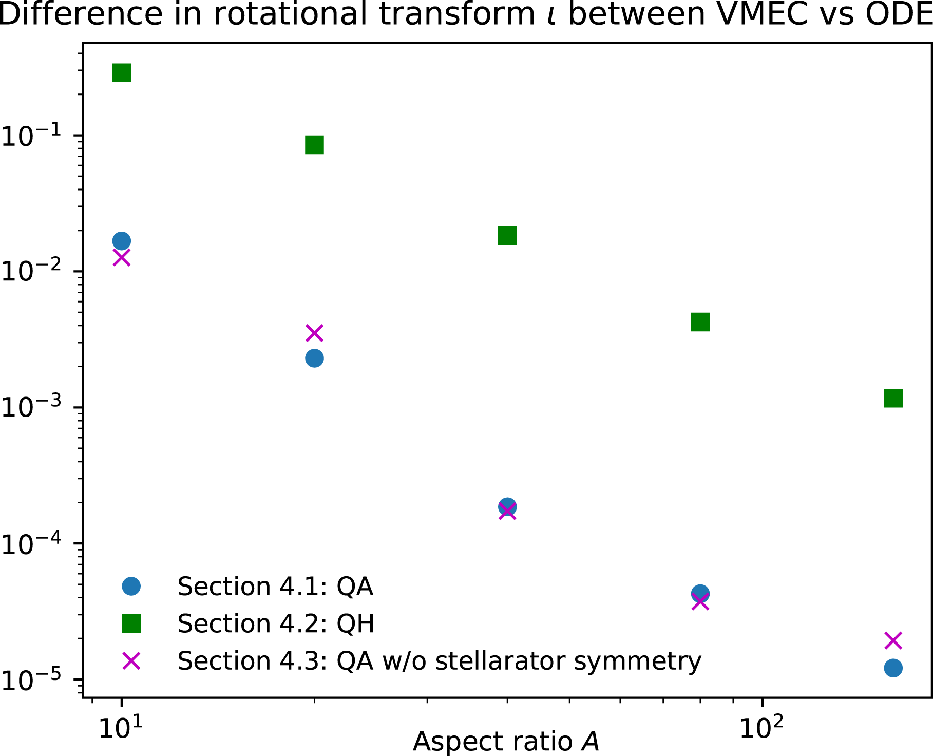
Figure 4 includes a point for the quasi-axisymmetric design NCSX, which was obtained using conventional optimization. The NCSX point falls below the trend line, so it evidently has a somewhat better quality of quasisymmetry for its aspect ratio than the configurations constructed here.

Figure 4. For all three examples presented in § 5, the symmetry-breaking Fourier components scale as
 $A^{-2}$
as predicted by theory.
$A^{-2}$
as predicted by theory.

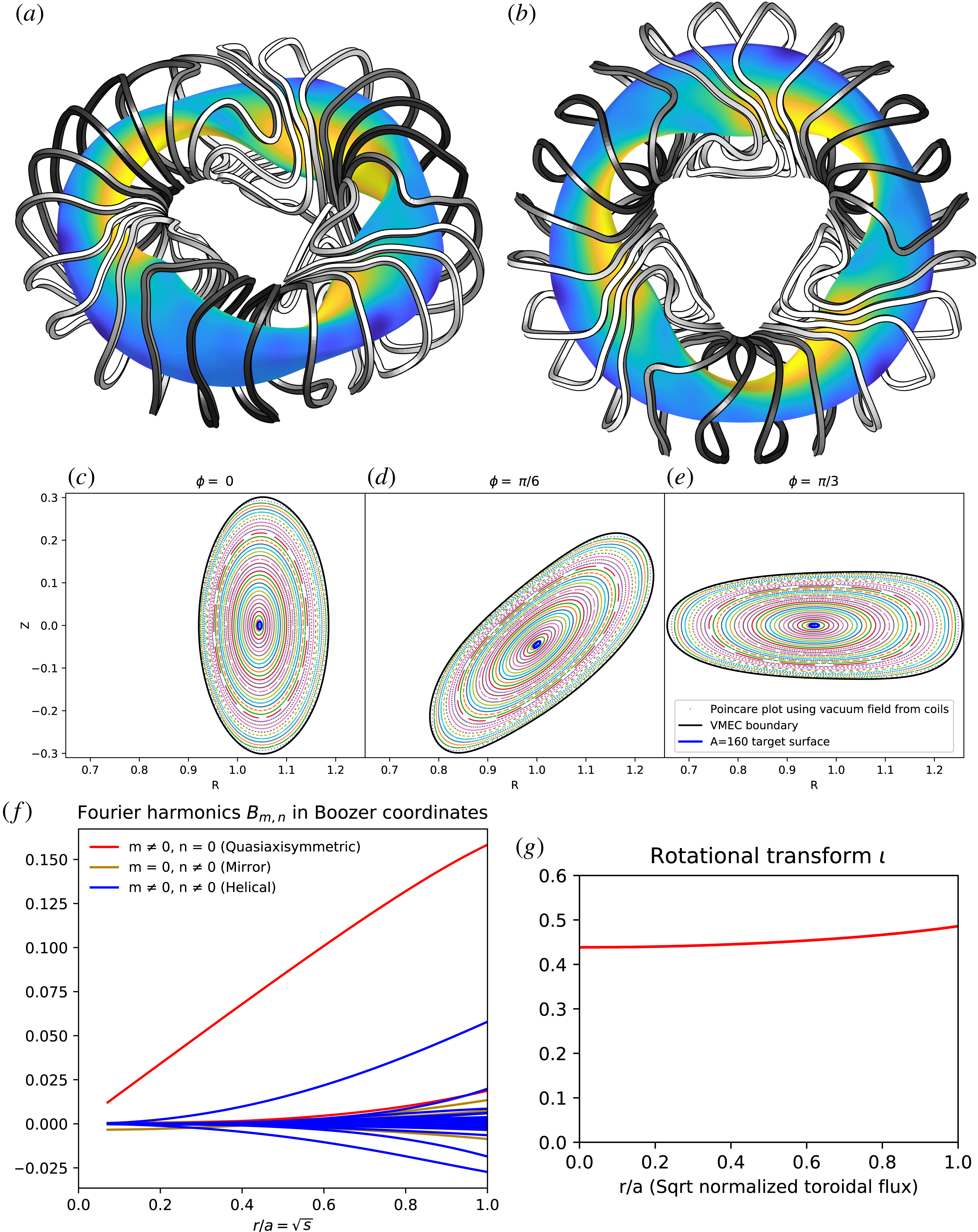
Figure 6. The aspect ratio 5 quasi-axisymmetic stellarator constructed by the procedure of § 4.4, using no optimization (aside from the REGCOIL linear least-squares problem). (a,b) Colour indicates
 $B$
on the outermost flux surface, and the four unique coil shapes are shown with four shades of grey. (c–e) Poincaré plots computed from the vacuum field of the coils, demonstrating good flux surfaces out to aspect ratio 5, at three toroidal angles. (f) Boozer spectrum, demonstrating the quasi-axisymmetric mode is dominant. (g) Profile of
$B$
on the outermost flux surface, and the four unique coil shapes are shown with four shades of grey. (c–e) Poincaré plots computed from the vacuum field of the coils, demonstrating good flux surfaces out to aspect ratio 5, at three toroidal angles. (f) Boozer spectrum, demonstrating the quasi-axisymmetric mode is dominant. (g) Profile of
 $\unicode[STIX]{x1D704}$
.
$\unicode[STIX]{x1D704}$
.
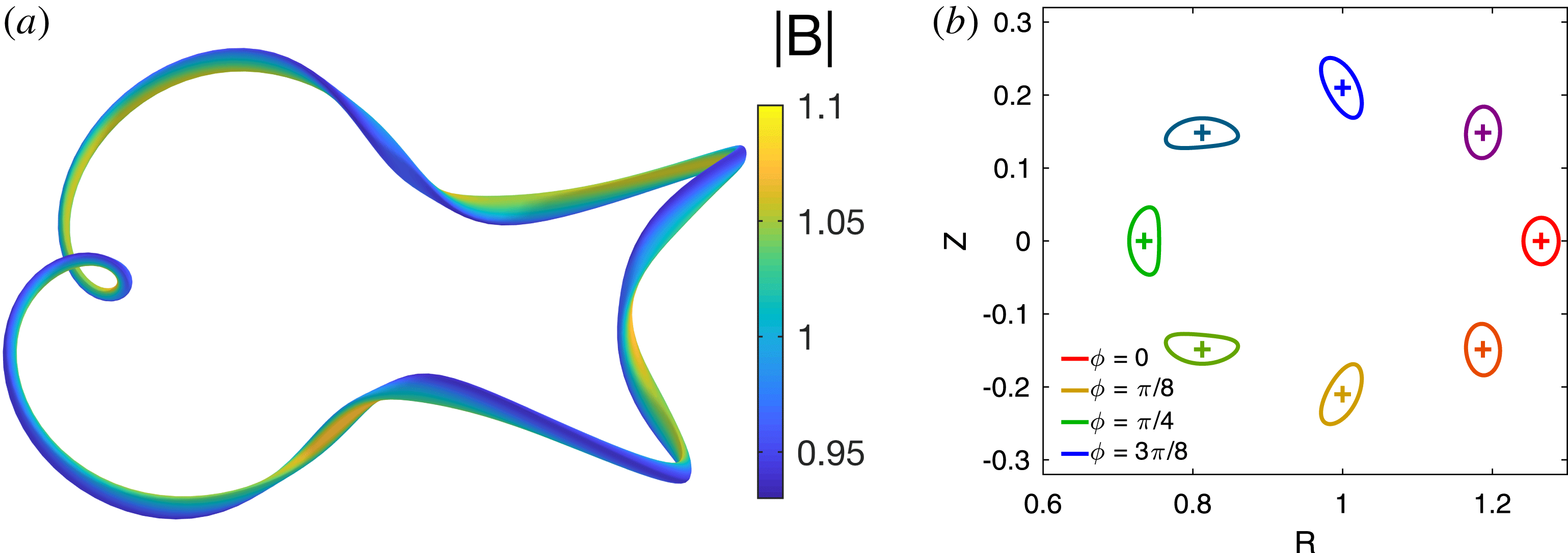
Figure 7. Quasi-helical symmetry example. (a) Flux surface shape computed by the procedure of §§ 3 and 4.2, taking aspect ratio
 $=$
40, showing
$=$
40, showing
 $|B|$
computed by VMEC. (b) Cross-sections of the flux surfaces at equally spaced values of
$|B|$
computed by VMEC. (b) Cross-sections of the flux surfaces at equally spaced values of
 $\unicode[STIX]{x1D719}$
, with
$\unicode[STIX]{x1D719}$
, with
 $+$
signs denoting the magnetic axis.
$+$
signs denoting the magnetic axis.
For a different approach to constructing a finite-aspect-ratio geometry from the high-aspect-ratio theory, an example of the outward extrapolation method of § 4.4 is shown in figure 6, again using the input axis shape (5.1). First, an aspect ratio 160 shape is generated by the method of § 4.1. Coil shapes to produce this magnetic surface shape are then calculated using the REGCOIL method (Landreman Reference Landreman2017). For this method, a coil winding surface is chosen by taking an aspect ratio 5 surface constructed using the method of § 4.1, and expanding uniformly outward by one quarter of the average major radius. REGCOIL’s regularization parameter is chosen to be the smallest value for which there are no saddle coils, i.e. there are no local maxima or minima in the current potential. Next, 24 coil shapes (four unique shapes, each repeated six times) are identified from uniformly spaced contours of the current potential. A Poincaré plot of the vacuum field produced by these coils (figure 6
c–e) shows that good flux surfaces exist out to an aspect ratio of 5.0 (using VMEC’s definition of the major and minor radius). The Fourier amplitudes of
 $B$
in Boozer coordinates are shown in figure 6(f), showing the quasi-axisymmetric term is dominant, as desired. Again the largest symmetry-breaking mode at the edge is the mode
$B$
in Boozer coordinates are shown in figure 6(f), showing the quasi-axisymmetric term is dominant, as desired. Again the largest symmetry-breaking mode at the edge is the mode
 $(m,n)=(2,-3)$
. The symmetry-breaking harmonics reach a rather sizeable amplitude at the last closed flux surface, and no effort has been made to achieve other desirable physics properties such as a high magnetohydrodynamic
$(m,n)=(2,-3)$
. The symmetry-breaking harmonics reach a rather sizeable amplitude at the last closed flux surface, and no effort has been made to achieve other desirable physics properties such as a high magnetohydrodynamic
 $\unicode[STIX]{x1D6FD}$
limit. However, this configuration required very little computational effort to compute, compared to the hundreds or thousands of VMEC computations required for conventional optimization, and it could serve as a useful initial condition for conventional optimization.
$\unicode[STIX]{x1D6FD}$
limit. However, this configuration required very little computational effort to compute, compared to the hundreds or thousands of VMEC computations required for conventional optimization, and it could serve as a useful initial condition for conventional optimization.
5.2 Quasi-helical symmetry
For an example of quasi-helical symmetry, we consider the magnetic axis shape
 $$\begin{eqnarray}R_{0}(\unicode[STIX]{x1D719})=1+0.265\cos (4\unicode[STIX]{x1D719}),\quad z_{0}(\unicode[STIX]{x1D719})=-0.21\sin (4\unicode[STIX]{x1D719}).\end{eqnarray}$$
For this curve, the normal vector rotates poloidally in each field period, so solutions have quasi-helical symmetry rather than quasi-axisymmetry. We also choose
 $\bar{\unicode[STIX]{x1D702}}=-2.25$
and
$\bar{\unicode[STIX]{x1D702}}=-2.25$
and
 $\unicode[STIX]{x1D70E}(0)=0$
. For these parameters, the numerical procedure of §§ 3–4.1 yields a rotational transform
$\unicode[STIX]{x1D70E}(0)=0$
. For these parameters, the numerical procedure of §§ 3–4.1 yields a rotational transform
 $\unicode[STIX]{x1D704}=1.93$
, and the maximum flux surface elongation in the
$\unicode[STIX]{x1D704}=1.93$
, and the maximum flux surface elongation in the
 $R$
–
$R$
–
 $z$
plane is found to be 2.52.
$z$
plane is found to be 2.52.
The flux surfaces for aspect ratio 40, computed using the method of § 4.2, are shown in figure 7. Due to the strongly shaped axis in this example, the flux surface cross-sections in the
 $R$
–
$R$
–
 $z$
plane become visibly different from ellipses even at this high aspect ratio. Note that the cross-sections in the plane perpendicular to the magnetic axis are perfectly elliptical, and the cross-sections in the
$z$
plane become visibly different from ellipses even at this high aspect ratio. Note that the cross-sections in the plane perpendicular to the magnetic axis are perfectly elliptical, and the cross-sections in the
 $R$
–
$R$
–
 $z$
plane approach ellipses as the aspect ratio is raised. The spectra of
$z$
plane approach ellipses as the aspect ratio is raised. The spectra of
 $B$
in Boozer coordinates for aspect ratios 40 and 160 are shown in figure 8. The largest symmetry-breaking mode at the edge is the mode
$B$
in Boozer coordinates for aspect ratios 40 and 160 are shown in figure 8. The largest symmetry-breaking mode at the edge is the mode
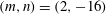 $(m,n)=(2,-16)$
.
$(m,n)=(2,-16)$
.
As pointed out by Garren & Boozer (Reference Garren and Boozer1991a
), the relevant ratio for breaking of quasisymmetry is the minor radius divided by the scale length of the magnetic axis’ Frenet–Serret frame (e.g.
 $1/\unicode[STIX]{x1D705}$
,
$1/\unicode[STIX]{x1D705}$
,
 $1/\unicode[STIX]{x1D70F}$
), not the conventional aspect ratio. For axis shapes consistent with quasi-helical symmetry, where the normal vector rotates about the axis, the scale lengths of the axis Frenet–Serret frame are smaller than for axes consistent with quasi-axisymmetry at comparable major radius. Therefore, quasi-helical symmetry is limited to higher conventional aspect ratios than quasi-axisymmetry. This trend is apparent in a comparison of the examples of §§ 5.1–5.2. The peak axis curvature and torsion are approximately twice as large in the latter compared to the former, and this ratio is squared in the symmetry breaking. Indeed, figure 3(a) for quasi-axisymmetry at aspect ratio 10 has comparable symmetry breaking to figure 8(a) for quasi-helical symmetry at aspect ratio 40.
$1/\unicode[STIX]{x1D70F}$
), not the conventional aspect ratio. For axis shapes consistent with quasi-helical symmetry, where the normal vector rotates about the axis, the scale lengths of the axis Frenet–Serret frame are smaller than for axes consistent with quasi-axisymmetry at comparable major radius. Therefore, quasi-helical symmetry is limited to higher conventional aspect ratios than quasi-axisymmetry. This trend is apparent in a comparison of the examples of §§ 5.1–5.2. The peak axis curvature and torsion are approximately twice as large in the latter compared to the former, and this ratio is squared in the symmetry breaking. Indeed, figure 3(a) for quasi-axisymmetry at aspect ratio 10 has comparable symmetry breaking to figure 8(a) for quasi-helical symmetry at aspect ratio 40.
Figure 8. Fourier amplitudes
 $B_{m,n}(r)$
of the magnetic field magnitude
$B_{m,n}(r)$
of the magnetic field magnitude
 $B(r,\unicode[STIX]{x1D703},\unicode[STIX]{x1D711})$
computed by BOOZ_XFORM, for the quasi-helically symmetric configuration of § 5.2.
$B(r,\unicode[STIX]{x1D703},\unicode[STIX]{x1D711})$
computed by BOOZ_XFORM, for the quasi-helically symmetric configuration of § 5.2.
Figure 4 includes a point for the quasi-helically symmetric experiment HSX, which was designed using conventional optimization. (Coil ripple is not included for the HSX and NCSX configurations in the figure; the values of
 $S$
for HSX and NCSX are nearly unchanged on the scale of the figure if coil ripple is included.) HSX has symmetry breaking that is an order of magnitude smaller than the configuration generated here at comparable aspect ratio. The fact that conventional optimization results in lower symmetry breaking than the construction here is not surprising, given that the construction is limited to producing shapes with elliptical cross-section.
$S$
for HSX and NCSX are nearly unchanged on the scale of the figure if coil ripple is included.) HSX has symmetry breaking that is an order of magnitude smaller than the configuration generated here at comparable aspect ratio. The fact that conventional optimization results in lower symmetry breaking than the construction here is not surprising, given that the construction is limited to producing shapes with elliptical cross-section.
Figure 9. Quasi-axisymmetric stellarator without stellarator symmetry. (a) Flux surface shape computed by the procedure of §§ 3 and 4.1, taking aspect ratio
 $=$
10, showing
$=$
10, showing
 $|B|$
computed by VMEC. (b) Cross-sections of the flux surfaces at equally spaced values of
$|B|$
computed by VMEC. (b) Cross-sections of the flux surfaces at equally spaced values of
 $\unicode[STIX]{x1D719}$
, with
$\unicode[STIX]{x1D719}$
, with
 $+$
signs denoting the magnetic axis.
$+$
signs denoting the magnetic axis.
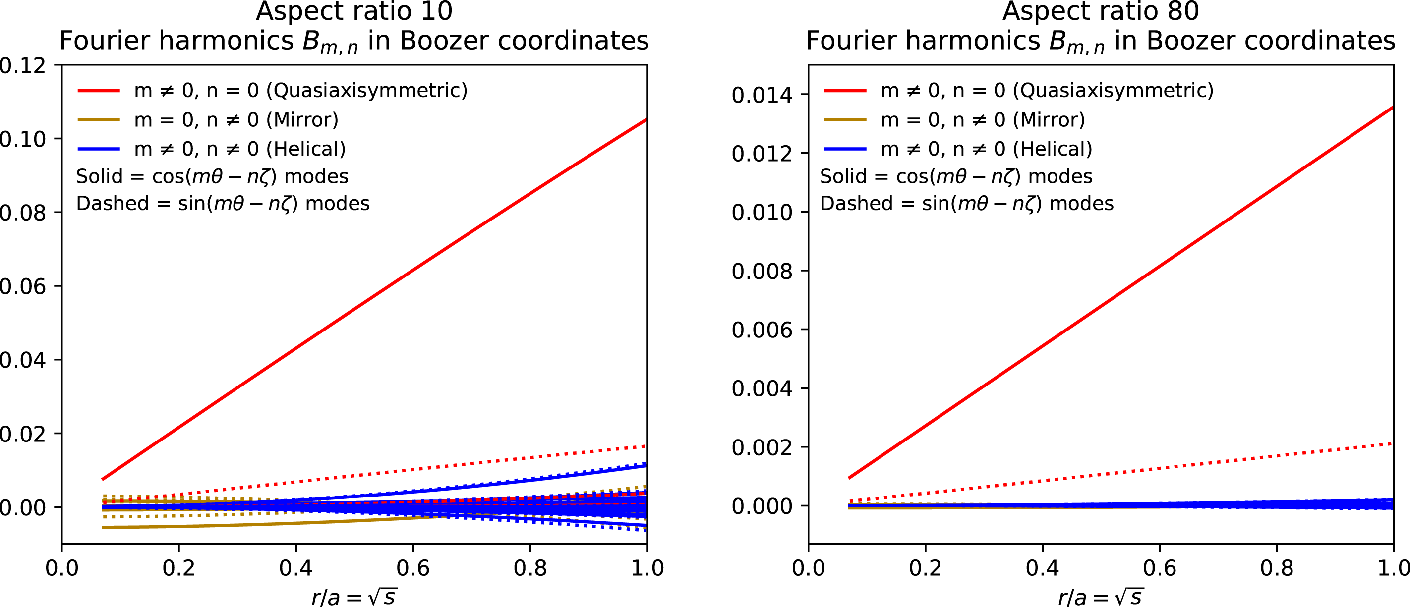
Figure 10. Fourier amplitudes
 $B_{m,n}(r)$
of the magnetic field magnitude
$B_{m,n}(r)$
of the magnetic field magnitude
 $B(r,\unicode[STIX]{x1D703},\unicode[STIX]{x1D711})$
computed by BOOZ_XFORM, for the non-stellarator-symmetric quasi-axisymmetric configuration of § 5.3.
$B(r,\unicode[STIX]{x1D703},\unicode[STIX]{x1D711})$
computed by BOOZ_XFORM, for the non-stellarator-symmetric quasi-axisymmetric configuration of § 5.3.
5.3 Case without stellarator symmetry
There is no reason a stellarator with quasisymmetry must also possess stellarator symmetry. For instance, a tokamak with a single null is quasi-axisymmetric but not stellarator symmetric. Plasma shapes that lack stellarator symmetry are of interest since the turbulent momentum flux is predicted to be larger by a factor
 ${\sim}1/\unicode[STIX]{x1D70C}_{\ast }$
than in stellarator-symmetric shapes, meaning the intrinsic rotation is larger (Peeters & Angioni Reference Peeters and Angioni2005; Parra, Barnes & Peeters Reference Parra, Barnes and Peeters2011; Sugama et al.
Reference Sugama, Watanabe, Nunami and Nishimura2011). The resulting rotation and/or rotation shear may improve plasma stability. While quasisymmetry reduces the strong damping of flows otherwise typical of stellarators, significant flow still requires a drive, and turbulent momentum transport associated with broken stellarator symmetry could provide such a drive. In the model considered here, stellarator symmetry can be broken by specifying a non-stellarator-symmetric axis shape, or by specifying a non-zero
${\sim}1/\unicode[STIX]{x1D70C}_{\ast }$
than in stellarator-symmetric shapes, meaning the intrinsic rotation is larger (Peeters & Angioni Reference Peeters and Angioni2005; Parra, Barnes & Peeters Reference Parra, Barnes and Peeters2011; Sugama et al.
Reference Sugama, Watanabe, Nunami and Nishimura2011). The resulting rotation and/or rotation shear may improve plasma stability. While quasisymmetry reduces the strong damping of flows otherwise typical of stellarators, significant flow still requires a drive, and turbulent momentum transport associated with broken stellarator symmetry could provide such a drive. In the model considered here, stellarator symmetry can be broken by specifying a non-stellarator-symmetric axis shape, or by specifying a non-zero
 $\unicode[STIX]{x1D70E}(0)$
, or both. Here we present an example with both sources of symmetry breaking. We take the magnetic axis shape to be
$\unicode[STIX]{x1D70E}(0)$
, or both. Here we present an example with both sources of symmetry breaking. We take the magnetic axis shape to be
 $$\begin{eqnarray}R_{0}(\unicode[STIX]{x1D719})=1+0.042\cos (3\unicode[STIX]{x1D719}),\quad z_{0}(\unicode[STIX]{x1D719})=-0.042\sin (3\unicode[STIX]{x1D719})-0.025\cos (3\unicode[STIX]{x1D719}),\end{eqnarray}$$
with
 $\bar{\unicode[STIX]{x1D702}}=-1.1$
and
$\bar{\unicode[STIX]{x1D702}}=-1.1$
and
 $\unicode[STIX]{x1D70E}(0)=-0.6$
. For these parameters, the numerical procedure above yields a rotational transform
$\unicode[STIX]{x1D70E}(0)=-0.6$
. For these parameters, the numerical procedure above yields a rotational transform
 $\unicode[STIX]{x1D704}=0.311$
, and the maximum flux surface elongation in the
$\unicode[STIX]{x1D704}=0.311$
, and the maximum flux surface elongation in the
 $R$
–
$R$
–
 $z$
plane is found to be 3.29. The flux surface shape for
$z$
plane is found to be 3.29. The flux surface shape for
 $A=10$
is displayed in figure 9, and the Boozer spectra for
$A=10$
is displayed in figure 9, and the Boozer spectra for
 $A=10$
and
$A=10$
and
 $A=80$
are shown in figure 10. In figure 10, it can be seen that
$A=80$
are shown in figure 10. In figure 10, it can be seen that
 $B$
has a significant
$B$
has a significant
 $\sin \unicode[STIX]{x1D703}$
component (red dotted line) which is not stellarator symmetric but which preserves quasi-axisymmetry. As with the stellarator-symmetric quasi-axisymmetric example, the largest symmetry-breaking mode at the edge is the mode
$\sin \unicode[STIX]{x1D703}$
component (red dotted line) which is not stellarator symmetric but which preserves quasi-axisymmetry. As with the stellarator-symmetric quasi-axisymmetric example, the largest symmetry-breaking mode at the edge is the mode
 $(m,n)=(2,-3)$
. The
$(m,n)=(2,-3)$
. The
 $1/A^{2}$
scaling of the quasisymmetry-breaking harmonics is again plotted in figure 4, and the convergence of the VMEC rotational transform to the predicted value as
$1/A^{2}$
scaling of the quasisymmetry-breaking harmonics is again plotted in figure 4, and the convergence of the VMEC rotational transform to the predicted value as
 $A\rightarrow \infty$
is shown in figure 5. Generally the properties of this family of configurations are quite similar to the stellarator-symmetric and quasi-axisymmetric configurations of § 5.1.
$A\rightarrow \infty$
is shown in figure 5. Generally the properties of this family of configurations are quite similar to the stellarator-symmetric and quasi-axisymmetric configurations of § 5.1.
6 Discussion and conclusions
While quasisymmetric stellarator shapes have been found previously by applying black-box optimization methods to minimize the departure from quasisymmetry, such methods are computationally demanding and do not provide comprehensive information about the landscape of all possible solutions. Here we have demonstrated a complementary approach in which quasisymmetric stellarator shapes can be parameterized and computed extremely rapidly (
 ${<}1~\text{ms}$
on a laptop), enabling exhaustive high-resolution parameter scans and insight into the size of the solution space. We have demonstrated that this approach is a practical method to generate configurations that can be examined numerically with VMEC and other physics codes. As part of this demonstration, we have shown using BOOZ_XFORM that the Boozer coordinate Fourier spectra of the resulting equilibria are indeed dominated by a single helicity. We have further demonstrated that the symmetry-breaking harmonics scale as
${<}1~\text{ms}$
on a laptop), enabling exhaustive high-resolution parameter scans and insight into the size of the solution space. We have demonstrated that this approach is a practical method to generate configurations that can be examined numerically with VMEC and other physics codes. As part of this demonstration, we have shown using BOOZ_XFORM that the Boozer coordinate Fourier spectra of the resulting equilibria are indeed dominated by a single helicity. We have further demonstrated that the symmetry-breaking harmonics scale as
 $r^{2}$
as expected.
$r^{2}$
as expected.
Although the ‘optimization-free’ approach here requires solving a nonlinear equation (2.7), the numerical solution is extremely robust since the problem can be formulated so a unique solution is guaranteed to exist. As proved in appendix A, every magnetic axis shape with non-vanishing curvature admits an infinity of (first-order) quasisymmetric flux surface shapes surrounding it, each labelled by the three numbers
 $\bar{\unicode[STIX]{x1D702}}$
,
$\bar{\unicode[STIX]{x1D702}}$
,
 $I_{2}$
and
$I_{2}$
and
 $\unicode[STIX]{x1D70E}(0)$
. Given any values for these three numbers, as long as
$\unicode[STIX]{x1D70E}(0)$
. Given any values for these three numbers, as long as
 $\bar{\unicode[STIX]{x1D702}}\neq 0$
, and given any axis shape for which the curvature does not vanish, there is exactly one first-order quasisymmetric shape (as a function of
$\bar{\unicode[STIX]{x1D702}}\neq 0$
, and given any axis shape for which the curvature does not vanish, there is exactly one first-order quasisymmetric shape (as a function of
 $r$
). However, much of this solution space is not interesting since the elongation of the surfaces is impractically high. The space of stellarator-symmetric solutions is significantly smaller than the space of all solutions both because the space of axis shapes is restricted and also since
$r$
). However, much of this solution space is not interesting since the elongation of the surfaces is impractically high. The space of stellarator-symmetric solutions is significantly smaller than the space of all solutions both because the space of axis shapes is restricted and also since
 $\unicode[STIX]{x1D70E}(0)$
must be 0.
$\unicode[STIX]{x1D70E}(0)$
must be 0.
While the calculations here are limited to high aspect ratio, any stellarator with a low-aspect-ratio boundary will have a region close to the magnetic axis in which the local aspect ratio is high. Hence the results here describe the core of any quasisymmetric stellarator, even those with low aspect ratio at the plasma boundary. The observed accuracy of the solutions constructed here is consistent with the popular wisdom that good quasi-axisymmetry can be achieved at much lower aspect ratio than quasi-helical symmetry. It is likely that by extending the method here to second order in
 $r$
, using equations in the appendix of Garren & Boozer (Reference Garren and Boozer1991b
), the accuracy of these parameterized solutions could be extended to lower aspect ratio.
$r$
, using equations in the appendix of Garren & Boozer (Reference Garren and Boozer1991b
), the accuracy of these parameterized solutions could be extended to lower aspect ratio.
Acknowledgements
We are grateful to H. Weitzner for pointing out the possibility of singularity in (A 1). The idea of a non-stellarator-symmetric quasisymmetric stellarator was suggested by G. Hammett. This work was supported by the U.S. Department of Energy, Office of Science, Office of Fusion Energy Science, under award nos. DE-FG02-93ER54197 and DE-FG02-86ER53223. This work was also supported by a grant from the Simons Foundation (560651, ML).
Appendix A. Existence and uniqueness of solutions to the ordinary differential equation
The problem for first-order quasisymmetry (2.7) can be stated as
 $$\begin{eqnarray}\frac{\text{d}\unicode[STIX]{x1D70E}}{\text{d}\unicode[STIX]{x1D711}}+\unicode[STIX]{x1D704}(P+\unicode[STIX]{x1D70E}^{2})+Q=0,\quad \unicode[STIX]{x1D70E}(0)\text{ given},\end{eqnarray}$$
where
 $\unicode[STIX]{x1D70E}(\unicode[STIX]{x1D711})$
,
$\unicode[STIX]{x1D70E}(\unicode[STIX]{x1D711})$
,
 $P(\unicode[STIX]{x1D711})$
and
$P(\unicode[STIX]{x1D711})$
and
 $Q(\unicode[STIX]{x1D711})$
are
$Q(\unicode[STIX]{x1D711})$
are
 $2\unicode[STIX]{x03C0}$
-periodic functions,
$2\unicode[STIX]{x03C0}$
-periodic functions,
 $P>0$
, and
$P>0$
, and
 $\unicode[STIX]{x1D704}$
and
$\unicode[STIX]{x1D704}$
and
 $\unicode[STIX]{x1D70E}(0)$
are constants. (Without loss of generality, the shift
$\unicode[STIX]{x1D70E}(0)$
are constants. (Without loss of generality, the shift
 $-N$
to
$-N$
to
 $\unicode[STIX]{x1D704}$
is dropped in this appendix to simplify notation.) Here we prove that for given
$\unicode[STIX]{x1D704}$
is dropped in this appendix to simplify notation.) Here we prove that for given
 $P$
,
$P$
,
 $Q$
and
$Q$
and
 $\unicode[STIX]{x1D70E}(0)$
, assuming that
$\unicode[STIX]{x1D70E}(0)$
, assuming that
 $P$
and
$P$
and
 $Q$
are integrable and bounded, a periodic solution
$Q$
are integrable and bounded, a periodic solution
 $\{\unicode[STIX]{x1D704},\;\unicode[STIX]{x1D70E}(\unicode[STIX]{x1D711})\}$
to (A 1) exists and it is unique.
$\{\unicode[STIX]{x1D704},\;\unicode[STIX]{x1D70E}(\unicode[STIX]{x1D711})\}$
to (A 1) exists and it is unique.
Note that if the problem is posed instead with
 $\unicode[STIX]{x1D704}$
as given and
$\unicode[STIX]{x1D704}$
as given and
 $\unicode[STIX]{x1D70E}(0)$
as part of the solution, rather than the other way around, then there may be zero, one or two solutions. In this alternative formulation there can never be more than two solutions (Pliss Reference Pliss1966, p. 102).
$\unicode[STIX]{x1D70E}(0)$
as part of the solution, rather than the other way around, then there may be zero, one or two solutions. In this alternative formulation there can never be more than two solutions (Pliss Reference Pliss1966, p. 102).

Figure 11. (a) Solutions of the ODE (A 1), interpreted as an initial value problem, for
 $P=2+\sin (2\unicode[STIX]{x1D711})$
,
$P=2+\sin (2\unicode[STIX]{x1D711})$
,
 $Q=1+3\cos \unicode[STIX]{x1D711}$
,
$Q=1+3\cos \unicode[STIX]{x1D711}$
,
 $\unicode[STIX]{x1D70E}(0)=2$
and various
$\unicode[STIX]{x1D70E}(0)=2$
and various
 $\unicode[STIX]{x1D704}\in [-1,1]$
. (b) Demonstration that
$\unicode[STIX]{x1D704}\in [-1,1]$
. (b) Demonstration that
 $\unicode[STIX]{x0394}(\unicode[STIX]{x1D704})=\unicode[STIX]{x1D70E}(2\unicode[STIX]{x03C0})-\unicode[STIX]{x1D70E}(0)$
is a monotonically decreasing function of
$\unicode[STIX]{x0394}(\unicode[STIX]{x1D704})=\unicode[STIX]{x1D70E}(2\unicode[STIX]{x03C0})-\unicode[STIX]{x1D70E}(0)$
is a monotonically decreasing function of
 $\unicode[STIX]{x1D704}$
, and illustration of the function
$\unicode[STIX]{x1D704}$
, and illustration of the function
 $\bar{\unicode[STIX]{x0394}}(\unicode[STIX]{x1D704})$
of § A.4, for the same parameters as (a).
$\bar{\unicode[STIX]{x0394}}(\unicode[STIX]{x1D704})$
of § A.4, for the same parameters as (a).
A.1 Uniqueness
Returning to the original formulation of (A 1) with
 $\unicode[STIX]{x1D70E}(0)$
as an input and
$\unicode[STIX]{x1D70E}(0)$
as an input and
 $\unicode[STIX]{x1D704}$
as an output, we will first prove that no more than one solution can exist. For the moment, we relax the requirement that
$\unicode[STIX]{x1D704}$
as an output, we will first prove that no more than one solution can exist. For the moment, we relax the requirement that
 $\unicode[STIX]{x1D70E}(\unicode[STIX]{x1D711})$
be periodic, so that for any given
$\unicode[STIX]{x1D70E}(\unicode[STIX]{x1D711})$
be periodic, so that for any given
 $\unicode[STIX]{x1D704}$
, equation (A 1) becomes an initial value problem, which has a unique, finite, and generally non-periodic solution
$\unicode[STIX]{x1D704}$
, equation (A 1) becomes an initial value problem, which has a unique, finite, and generally non-periodic solution
 $\unicode[STIX]{x1D70E}(\unicode[STIX]{x1D711})$
in some neighbourhood of
$\unicode[STIX]{x1D70E}(\unicode[STIX]{x1D711})$
in some neighbourhood of
 $\unicode[STIX]{x1D711}=0$
. Solutions for a particular choice of
$\unicode[STIX]{x1D711}=0$
. Solutions for a particular choice of
 $P$
,
$P$
,
 $Q$
and
$Q$
and
 $\unicode[STIX]{x1D70E}(0)$
are shown in figure 11(a). Note that the solution of this initial value problem may not extend all the way to
$\unicode[STIX]{x1D70E}(0)$
are shown in figure 11(a). Note that the solution of this initial value problem may not extend all the way to
 $\unicode[STIX]{x1D711}=2\unicode[STIX]{x03C0}$
since it may diverge to
$\unicode[STIX]{x1D711}=2\unicode[STIX]{x03C0}$
since it may diverge to
 $\pm \infty$
beforehand, as can be seen from the analytic solution in the case of constant
$\pm \infty$
beforehand, as can be seen from the analytic solution in the case of constant
 $P$
and
$P$
and
 $Q$
:
$Q$
:
 $$\begin{eqnarray}\unicode[STIX]{x1D70E}(\unicode[STIX]{x1D711})=-\sqrt{(Q+P\unicode[STIX]{x1D704})/\unicode[STIX]{x1D704}}\tan \left(\unicode[STIX]{x1D711}\sqrt{(Q+P\unicode[STIX]{x1D704})\unicode[STIX]{x1D704}}-\tan ^{-1}\left(\unicode[STIX]{x1D70E}(0)\sqrt{\unicode[STIX]{x1D704}/(Q+P\unicode[STIX]{x1D704})}\right)\right).\end{eqnarray}$$
Returning to the case of general
 $P>0$
and
$P>0$
and
 $Q$
, suppose
$Q$
, suppose
 $\unicode[STIX]{x1D70E}_{0}(\unicode[STIX]{x1D711})$
is the solution to the initial value problem for
$\unicode[STIX]{x1D70E}_{0}(\unicode[STIX]{x1D711})$
is the solution to the initial value problem for
 $\unicode[STIX]{x1D704}=\unicode[STIX]{x1D704}_{0}$
, and
$\unicode[STIX]{x1D704}=\unicode[STIX]{x1D704}_{0}$
, and
 $\unicode[STIX]{x1D70E}_{1}(\unicode[STIX]{x1D711})$
is the solution for
$\unicode[STIX]{x1D70E}_{1}(\unicode[STIX]{x1D711})$
is the solution for
 $\unicode[STIX]{x1D704}=\unicode[STIX]{x1D704}_{1}$
. Subtracting (A 1) for these two solutions,
$\unicode[STIX]{x1D704}=\unicode[STIX]{x1D704}_{1}$
. Subtracting (A 1) for these two solutions,
 $$\begin{eqnarray}\displaystyle 0 & = & \displaystyle \frac{\text{d}(\unicode[STIX]{x1D70E}_{1}-\unicode[STIX]{x1D70E}_{0})}{\text{d}\unicode[STIX]{x1D711}}+(\unicode[STIX]{x1D704}_{1}-\unicode[STIX]{x1D704}_{0})P+\unicode[STIX]{x1D704}_{1}\unicode[STIX]{x1D70E}_{1}^{2}-\unicode[STIX]{x1D704}_{0}\unicode[STIX]{x1D70E}_{0}^{2},\nonumber\\ \displaystyle & = & \displaystyle \frac{\text{d}(\unicode[STIX]{x1D70E}_{1}-\unicode[STIX]{x1D70E}_{0})}{\text{d}\unicode[STIX]{x1D711}}+(\unicode[STIX]{x1D704}_{1}-\unicode[STIX]{x1D704}_{0})(P+\unicode[STIX]{x1D70E}_{0}^{2})+\unicode[STIX]{x1D704}_{1}(\unicode[STIX]{x1D70E}_{1}-\unicode[STIX]{x1D70E}_{0})(\unicode[STIX]{x1D70E}_{1}+\unicode[STIX]{x1D70E}_{0}).\end{eqnarray}$$
This equation may be integrated using an integrating factor to give
 $$\begin{eqnarray}\unicode[STIX]{x1D70E}_{1}(\unicode[STIX]{x1D711})-\unicode[STIX]{x1D70E}_{0}(\unicode[STIX]{x1D711})=-(\unicode[STIX]{x1D704}_{1}-\unicode[STIX]{x1D704}_{0})F(\unicode[STIX]{x1D711}),\end{eqnarray}$$
where
 $$\begin{eqnarray}\displaystyle F(\unicode[STIX]{x1D711}) & = & \displaystyle \exp \left(-\unicode[STIX]{x1D704}_{1}\int _{0}^{\unicode[STIX]{x1D711}}\,\text{d}\unicode[STIX]{x1D711}^{\prime }[\unicode[STIX]{x1D70E}_{1}(\unicode[STIX]{x1D711}^{\prime })+\unicode[STIX]{x1D70E}_{0}(\unicode[STIX]{x1D711}^{\prime })]\right)\nonumber\\ \displaystyle & & \displaystyle \times \,\int _{0}^{\unicode[STIX]{x1D711}}\,\text{d}\unicode[STIX]{x1D711}^{\prime \prime }[P(\unicode[STIX]{x1D711}^{\prime \prime })+\unicode[STIX]{x1D70E}_{0}^{2}(\unicode[STIX]{x1D711}^{\prime \prime })]\exp \left(\unicode[STIX]{x1D704}_{1}\int _{0}^{\unicode[STIX]{x1D711}^{\prime \prime }}\,\text{d}\unicode[STIX]{x1D711}^{\prime }[\unicode[STIX]{x1D70E}_{1}(\unicode[STIX]{x1D711}^{\prime })+\unicode[STIX]{x1D70E}_{0}(\unicode[STIX]{x1D711}^{\prime })]\right).\end{eqnarray}$$
Using
 $P>0$
it can be seen that
$P>0$
it can be seen that
 $F(\unicode[STIX]{x1D711})>0$
for any positive
$F(\unicode[STIX]{x1D711})>0$
for any positive
 $\unicode[STIX]{x1D711}$
for which the initial value solutions exist, so
$\unicode[STIX]{x1D711}$
for which the initial value solutions exist, so
 $\unicode[STIX]{x1D704}_{1}>\unicode[STIX]{x1D704}_{0}$
implies
$\unicode[STIX]{x1D704}_{1}>\unicode[STIX]{x1D704}_{0}$
implies
 $\unicode[STIX]{x1D70E}_{1}(\unicode[STIX]{x1D711})<\unicode[STIX]{x1D70E}_{0}(\unicode[STIX]{x1D711})$
. That is,
$\unicode[STIX]{x1D70E}_{1}(\unicode[STIX]{x1D711})<\unicode[STIX]{x1D70E}_{0}(\unicode[STIX]{x1D711})$
. That is,
 $\unicode[STIX]{x1D70E}(\unicode[STIX]{x1D711})$
is a strictly monotonically decreasing function of
$\unicode[STIX]{x1D70E}(\unicode[STIX]{x1D711})$
is a strictly monotonically decreasing function of
 $\unicode[STIX]{x1D704}$
at any
$\unicode[STIX]{x1D704}$
at any
 $\unicode[STIX]{x1D711}$
for which the initial value solution exists. This is true in particular at
$\unicode[STIX]{x1D711}$
for which the initial value solution exists. This is true in particular at
 $\unicode[STIX]{x1D711}=2\unicode[STIX]{x03C0}$
. Defining
$\unicode[STIX]{x1D711}=2\unicode[STIX]{x03C0}$
. Defining
 $\unicode[STIX]{x0394}(\unicode[STIX]{x1D704})=\unicode[STIX]{x1D70E}(2\unicode[STIX]{x03C0})-\unicode[STIX]{x1D70E}(0)$
(defined at any
$\unicode[STIX]{x0394}(\unicode[STIX]{x1D704})=\unicode[STIX]{x1D70E}(2\unicode[STIX]{x03C0})-\unicode[STIX]{x1D70E}(0)$
(defined at any
 $\unicode[STIX]{x1D704}$
for which the initial value solutions do extend to
$\unicode[STIX]{x1D704}$
for which the initial value solutions do extend to
 $2\unicode[STIX]{x03C0}$
), we then have
$2\unicode[STIX]{x03C0}$
), we then have
 $$\begin{eqnarray}\unicode[STIX]{x0394}(\unicode[STIX]{x1D704}_{1})-\unicode[STIX]{x0394}(\unicode[STIX]{x1D704}_{0})=-(\unicode[STIX]{x1D704}_{1}-\unicode[STIX]{x1D704}_{0})F(2\unicode[STIX]{x03C0}).\end{eqnarray}$$
Using
 $F>0$
,
$F>0$
,
 $\unicode[STIX]{x0394}(\unicode[STIX]{x1D704})$
is a strictly monotonically decreasing function. Figure 11(b) shows
$\unicode[STIX]{x0394}(\unicode[STIX]{x1D704})$
is a strictly monotonically decreasing function. Figure 11(b) shows
 $\unicode[STIX]{x0394}(\unicode[STIX]{x1D704})$
for the particular parameters of figure 11(a), and this monotonicity is apparent. Thus, no more than a single value of
$\unicode[STIX]{x0394}(\unicode[STIX]{x1D704})$
for the particular parameters of figure 11(a), and this monotonicity is apparent. Thus, no more than a single value of
 $\unicode[STIX]{x1D704}$
can exist for which
$\unicode[STIX]{x1D704}$
can exist for which
 $\unicode[STIX]{x0394}(\unicode[STIX]{x1D704})=0$
, corresponding to a periodic
$\unicode[STIX]{x0394}(\unicode[STIX]{x1D704})=0$
, corresponding to a periodic
 $\unicode[STIX]{x1D70E}(\unicode[STIX]{x1D711})$
.
$\unicode[STIX]{x1D70E}(\unicode[STIX]{x1D711})$
.
A.2 Bounded solutions
To prove that at least one solution to (A 1) exists, let us prove several intermediate results that will be needed, beginning with the following proposition. Suppose when
 $\unicode[STIX]{x1D704}=\unicode[STIX]{x1D704}_{0}$
, the initial value problem (A 1) with some given initial condition
$\unicode[STIX]{x1D704}=\unicode[STIX]{x1D704}_{0}$
, the initial value problem (A 1) with some given initial condition
 $\unicode[STIX]{x1D70E}(0)$
has a bounded solution
$\unicode[STIX]{x1D70E}(0)$
has a bounded solution
 $\unicode[STIX]{x1D70E}_{0}(\unicode[STIX]{x1D711})$
throughout
$\unicode[STIX]{x1D70E}_{0}(\unicode[STIX]{x1D711})$
throughout
 $\unicode[STIX]{x1D711}\in [0,2\unicode[STIX]{x03C0}]$
. Then there exists some
$\unicode[STIX]{x1D711}\in [0,2\unicode[STIX]{x03C0}]$
. Then there exists some
 $d>0$
such that for all
$d>0$
such that for all
 $\unicode[STIX]{x1D704}$
satisfying
$\unicode[STIX]{x1D704}$
satisfying
 $|\unicode[STIX]{x1D704}-\unicode[STIX]{x1D704}_{0}|<d$
, then
$|\unicode[STIX]{x1D704}-\unicode[STIX]{x1D704}_{0}|<d$
, then
 $\unicode[STIX]{x1D70E}$
solving the initial value problem (A 1) with
$\unicode[STIX]{x1D70E}$
solving the initial value problem (A 1) with
 $\unicode[STIX]{x1D704}$
and the same initial condition remains bounded throughout
$\unicode[STIX]{x1D704}$
and the same initial condition remains bounded throughout
 $\unicode[STIX]{x1D711}\in [0,2\unicode[STIX]{x03C0}]$
. In other words, for any
$\unicode[STIX]{x1D711}\in [0,2\unicode[STIX]{x03C0}]$
. In other words, for any
 $\unicode[STIX]{x1D704}_{0}$
that yields a solution that is non-singular, there are nearby values of
$\unicode[STIX]{x1D704}_{0}$
that yields a solution that is non-singular, there are nearby values of
 $\unicode[STIX]{x1D704}$
that also avoid singularity. Put yet another way, if
$\unicode[STIX]{x1D704}$
that also avoid singularity. Put yet another way, if
 ${\mathcal{B}}$
is the set of values of
${\mathcal{B}}$
is the set of values of
 $\unicode[STIX]{x1D704}$
that yield bounded solutions to the initial value problem (for a given
$\unicode[STIX]{x1D704}$
that yield bounded solutions to the initial value problem (for a given
 $\unicode[STIX]{x1D70E}(0)$
), then
$\unicode[STIX]{x1D70E}(0)$
), then
 ${\mathcal{B}}$
is open.
${\mathcal{B}}$
is open.
To prove this proposition, it is useful to consider the pair of solutions
 $\{\unicode[STIX]{x1D704}_{0},\unicode[STIX]{x1D70E}_{0}\}$
and
$\{\unicode[STIX]{x1D704}_{0},\unicode[STIX]{x1D70E}_{0}\}$
and
 $\{\unicode[STIX]{x1D704},\unicode[STIX]{x1D70E}\}$
which are both finite up to some
$\{\unicode[STIX]{x1D704},\unicode[STIX]{x1D70E}\}$
which are both finite up to some
 $\unicode[STIX]{x1D711}$
, and write (A 4) as
$\unicode[STIX]{x1D711}$
, and write (A 4) as
 $$\begin{eqnarray}\displaystyle & & \displaystyle [\unicode[STIX]{x1D70E}(\unicode[STIX]{x1D711})-\unicode[STIX]{x1D70E}_{0}(\unicode[STIX]{x1D711})]\exp \left(\unicode[STIX]{x1D704}\int _{0}^{\unicode[STIX]{x1D711}}\,\text{d}\unicode[STIX]{x1D711}^{\prime }[\unicode[STIX]{x1D70E}(\unicode[STIX]{x1D711}^{\prime })-\unicode[STIX]{x1D70E}_{0}(\unicode[STIX]{x1D711}^{\prime })]\right)\nonumber\\ \displaystyle & & \displaystyle \quad =(\unicode[STIX]{x1D704}_{0}-\unicode[STIX]{x1D704})\exp \left(-2\unicode[STIX]{x1D704}\int _{0}^{\unicode[STIX]{x1D711}}\,\text{d}\unicode[STIX]{x1D711}^{\prime }\unicode[STIX]{x1D70E}_{0}(\unicode[STIX]{x1D711}^{\prime })\right)\nonumber\\ \displaystyle & & \displaystyle \qquad \times \int _{0}^{\unicode[STIX]{x1D711}}\,\text{d}\unicode[STIX]{x1D711}^{\prime \prime }[P(\unicode[STIX]{x1D711}^{\prime \prime })+\unicode[STIX]{x1D70E}_{0}^{2}(\unicode[STIX]{x1D711}^{\prime \prime })]\exp \left(\unicode[STIX]{x1D704}\int _{0}^{\unicode[STIX]{x1D711}^{\prime \prime }}\,\text{d}\unicode[STIX]{x1D711}^{\prime }[\unicode[STIX]{x1D70E}(\unicode[STIX]{x1D711}^{\prime })+\unicode[STIX]{x1D70E}_{0}(\unicode[STIX]{x1D711}^{\prime })]\right).\end{eqnarray}$$
Recognizing the left-hand side as a total derivative
 $\unicode[STIX]{x1D704}^{-1}(\text{d}/\text{d}\unicode[STIX]{x1D711})\exp (\ldots )$
, and integrating,
$\unicode[STIX]{x1D704}^{-1}(\text{d}/\text{d}\unicode[STIX]{x1D711})\exp (\ldots )$
, and integrating,
 $$\begin{eqnarray}\displaystyle & & \displaystyle \exp \left(\unicode[STIX]{x1D704}\int _{0}^{\unicode[STIX]{x1D711}}\,\text{d}\unicode[STIX]{x1D711}^{\prime }[\unicode[STIX]{x1D70E}(\unicode[STIX]{x1D711}^{\prime })-\unicode[STIX]{x1D70E}_{0}(\unicode[STIX]{x1D711}^{\prime })]\right)=1+\unicode[STIX]{x1D704}(\unicode[STIX]{x1D704}_{0}-\unicode[STIX]{x1D704})\int _{0}^{\unicode[STIX]{x1D711}}\,\text{d}\unicode[STIX]{x1D711}^{\prime \prime \prime }\exp \left(-2\unicode[STIX]{x1D704}\int _{0}^{\unicode[STIX]{x1D711}^{\prime \prime \prime }}\,\text{d}\unicode[STIX]{x1D711}^{\prime }\unicode[STIX]{x1D70E}_{0}(\unicode[STIX]{x1D711}^{\prime })\right)\nonumber\\ \displaystyle & & \displaystyle \quad \times \int _{0}^{\unicode[STIX]{x1D711}^{\prime \prime \prime }}\,\text{d}\unicode[STIX]{x1D711}^{\prime \prime }[P(\unicode[STIX]{x1D711}^{\prime \prime })+\unicode[STIX]{x1D70E}_{0}^{2}(\unicode[STIX]{x1D711}^{\prime \prime })]\exp \left(\unicode[STIX]{x1D704}\int _{0}^{\unicode[STIX]{x1D711}^{\prime \prime }}\,\text{d}\unicode[STIX]{x1D711}^{\prime }[\unicode[STIX]{x1D70E}(\unicode[STIX]{x1D711}^{\prime })+\unicode[STIX]{x1D70E}_{0}(\unicode[STIX]{x1D711}^{\prime })]\right).\end{eqnarray}$$
We now consider three cases, depending on the sign of
 $\unicode[STIX]{x1D704}_{0}$
, beginning with the case
$\unicode[STIX]{x1D704}_{0}$
, beginning with the case
 $\unicode[STIX]{x1D704}_{0}<0$
. If
$\unicode[STIX]{x1D704}_{0}<0$
. If
 $\unicode[STIX]{x1D704}$
lies in
$\unicode[STIX]{x1D704}$
lies in
 $(\unicode[STIX]{x1D704}_{0},0)$
, then the fact that
$(\unicode[STIX]{x1D704}_{0},0)$
, then the fact that
 $\unicode[STIX]{x1D70E}$
is a monotonically decreasing function of
$\unicode[STIX]{x1D70E}$
is a monotonically decreasing function of
 $\unicode[STIX]{x1D704}$
at each
$\unicode[STIX]{x1D704}$
at each
 $\unicode[STIX]{x1D711}$
means that
$\unicode[STIX]{x1D711}$
means that
 $\unicode[STIX]{x1D70E}$
is bounded between
$\unicode[STIX]{x1D70E}$
is bounded between
 $\unicode[STIX]{x1D70E}_{0}$
and
$\unicode[STIX]{x1D70E}_{0}$
and
 $$\begin{eqnarray}\unicode[STIX]{x1D70E}_{Q}(\unicode[STIX]{x1D711})=\unicode[STIX]{x1D70E}(0)-\int _{0}^{\unicode[STIX]{x1D711}}\,\text{d}\unicode[STIX]{x1D711}^{\prime }Q(\unicode[STIX]{x1D711}^{\prime }),\end{eqnarray}$$
the solution of the initial value problem for
 $\unicode[STIX]{x1D704}=0$
. As
$\unicode[STIX]{x1D704}=0$
. As
 $\unicode[STIX]{x1D70E}_{0}$
and
$\unicode[STIX]{x1D70E}_{0}$
and
 $\unicode[STIX]{x1D70E}_{Q}$
are bounded throughout
$\unicode[STIX]{x1D70E}_{Q}$
are bounded throughout
 $[0,2\unicode[STIX]{x03C0}]$
,
$[0,2\unicode[STIX]{x03C0}]$
,
 $\unicode[STIX]{x1D70E}$
cannot be unbounded. On the other hand, if
$\unicode[STIX]{x1D70E}$
cannot be unbounded. On the other hand, if
 $\unicode[STIX]{x1D704}<\unicode[STIX]{x1D704}_{0}$
, then
$\unicode[STIX]{x1D704}<\unicode[STIX]{x1D704}_{0}$
, then
 $\unicode[STIX]{x1D70E}>\unicode[STIX]{x1D70E}_{0}$
and (A 8) imply
$\unicode[STIX]{x1D70E}>\unicode[STIX]{x1D70E}_{0}$
and (A 8) imply
 $$\begin{eqnarray}\exp \left(\unicode[STIX]{x1D704}\int _{0}^{\unicode[STIX]{x1D711}}\,\text{d}\unicode[STIX]{x1D711}^{\prime }[\unicode[STIX]{x1D70E}(\unicode[STIX]{x1D711}^{\prime })-\unicode[STIX]{x1D70E}_{0}(\unicode[STIX]{x1D711}^{\prime })]\right)>1-Y(\unicode[STIX]{x1D711}),\end{eqnarray}$$
where
 $$\begin{eqnarray}\displaystyle Y(\unicode[STIX]{x1D711}) & = & \displaystyle \unicode[STIX]{x1D704}(\unicode[STIX]{x1D704}-\unicode[STIX]{x1D704}_{0})\int _{0}^{\unicode[STIX]{x1D711}}\,\text{d}\unicode[STIX]{x1D711}^{\prime \prime \prime }\exp \left(-2\unicode[STIX]{x1D704}\int _{0}^{\unicode[STIX]{x1D711}^{\prime \prime \prime }}\,\text{d}\unicode[STIX]{x1D711}^{\prime }\unicode[STIX]{x1D70E}_{0}(\unicode[STIX]{x1D711}^{\prime })\right)\nonumber\\ \displaystyle & & \displaystyle \times \int _{0}^{\unicode[STIX]{x1D711}^{\prime \prime \prime }}\,\text{d}\unicode[STIX]{x1D711}^{\prime \prime }[P(\unicode[STIX]{x1D711}^{\prime \prime })+\unicode[STIX]{x1D70E}_{0}^{2}(\unicode[STIX]{x1D711}^{\prime \prime })]\exp \left(2\unicode[STIX]{x1D704}\int _{0}^{\unicode[STIX]{x1D711}^{\prime \prime }}\,\text{d}\unicode[STIX]{x1D711}^{\prime }\unicode[STIX]{x1D70E}_{0}(\unicode[STIX]{x1D711}^{\prime })\right).\end{eqnarray}$$
Note
 $Y>0$
. If
$Y>0$
. If
 $Y<1$
, then the reciprocal of (A 10) can be applied to (A 7) to obtain
$Y<1$
, then the reciprocal of (A 10) can be applied to (A 7) to obtain
 $$\begin{eqnarray}\displaystyle \unicode[STIX]{x1D70E}(\unicode[STIX]{x1D711}) & {<} & \displaystyle \unicode[STIX]{x1D70E}_{0}(\unicode[STIX]{x1D711})-\frac{\unicode[STIX]{x1D704}-\unicode[STIX]{x1D704}_{0}}{1-Y}\exp \left(-2\unicode[STIX]{x1D704}\int _{0}^{\unicode[STIX]{x1D711}}\,\text{d}\unicode[STIX]{x1D711}^{\prime }\unicode[STIX]{x1D70E}_{0}(\unicode[STIX]{x1D711}^{\prime })\right)\nonumber\\ \displaystyle & & \displaystyle \times \int _{0}^{\unicode[STIX]{x1D711}}\,\text{d}\unicode[STIX]{x1D711}^{\prime \prime }[P(\unicode[STIX]{x1D711}^{\prime \prime })+\unicode[STIX]{x1D70E}_{0}^{2}(\unicode[STIX]{x1D711}^{\prime \prime })]\exp \left(2\unicode[STIX]{x1D704}\int _{0}^{\unicode[STIX]{x1D711}^{\prime \prime }}\,\text{d}\unicode[STIX]{x1D711}^{\prime }\unicode[STIX]{x1D70E}_{0}(\unicode[STIX]{x1D711}^{\prime })\right).\end{eqnarray}$$
Therefore,
 $\unicode[STIX]{x1D70E}$
is bounded between
$\unicode[STIX]{x1D70E}$
is bounded between
 $\unicode[STIX]{x1D70E}_{0}$
and the right-hand side of (A 12), both of which are finite as long as
$\unicode[STIX]{x1D70E}_{0}$
and the right-hand side of (A 12), both of which are finite as long as
 $Y$
is bounded away from 1. To bound
$Y$
is bounded away from 1. To bound
 $Y$
, it is convenient to require
$Y$
, it is convenient to require
 $|\unicode[STIX]{x1D704}-\unicode[STIX]{x1D704}_{0}|<1$
, so
$|\unicode[STIX]{x1D704}-\unicode[STIX]{x1D704}_{0}|<1$
, so
 $$\begin{eqnarray}\unicode[STIX]{x1D704}_{0}\unicode[STIX]{x1D70E}_{0}-|\unicode[STIX]{x1D70E}_{0}|<\unicode[STIX]{x1D704}\unicode[STIX]{x1D70E}_{0}<\unicode[STIX]{x1D704}_{0}\unicode[STIX]{x1D70E}_{0}+|\unicode[STIX]{x1D70E}_{0}|,\end{eqnarray}$$
and
 $1/(-\unicode[STIX]{x1D704})>1/(1-\unicode[STIX]{x1D704}_{0})$
. Then requiring
$1/(-\unicode[STIX]{x1D704})>1/(1-\unicode[STIX]{x1D704}_{0})$
. Then requiring
 $|\unicode[STIX]{x1D704}-\unicode[STIX]{x1D704}_{0}|<d_{-}$
where
$|\unicode[STIX]{x1D704}-\unicode[STIX]{x1D704}_{0}|<d_{-}$
where
 $$\begin{eqnarray}\displaystyle d_{-} & = & \displaystyle \frac{1}{2(1-\unicode[STIX]{x1D704}_{0})}\min _{\unicode[STIX]{x1D711}}\left\{\int _{0}^{\unicode[STIX]{x1D711}}\,\text{d}\unicode[STIX]{x1D711}^{\prime \prime \prime }\exp \left(-2\int _{0}^{\unicode[STIX]{x1D711}^{\prime \prime \prime }}\,\text{d}\unicode[STIX]{x1D711}^{\prime }[\unicode[STIX]{x1D704}_{0}\unicode[STIX]{x1D70E}_{0}(\unicode[STIX]{x1D711}^{\prime })-|\unicode[STIX]{x1D70E}_{0}(\unicode[STIX]{x1D711}^{\prime })|]\right)\right.\nonumber\\ \displaystyle & & \displaystyle \times \left.\int _{0}^{\unicode[STIX]{x1D711}^{\prime \prime \prime }}\,\text{d}\unicode[STIX]{x1D711}^{\prime \prime }[P(\unicode[STIX]{x1D711}^{\prime \prime })+\unicode[STIX]{x1D70E}_{0}(\unicode[STIX]{x1D711}^{\prime \prime })]\exp \left(2\int _{0}^{\unicode[STIX]{x1D711}^{\prime \prime }}\,\text{d}\unicode[STIX]{x1D711}^{\prime }[\unicode[STIX]{x1D704}_{0}\unicode[STIX]{x1D70E}_{0}(\unicode[STIX]{x1D711}^{\prime })+|\unicode[STIX]{x1D70E}_{0}(\unicode[STIX]{x1D711}^{\prime })|]\!\right)\!\right\}^{-1}\!,\qquad\end{eqnarray}$$
where
 $\min _{\unicode[STIX]{x1D711}}$
indicates a minimum over
$\min _{\unicode[STIX]{x1D711}}$
indicates a minimum over
 $\unicode[STIX]{x1D711}\in [0,2\unicode[STIX]{x03C0}]$
, it follows that
$\unicode[STIX]{x1D711}\in [0,2\unicode[STIX]{x03C0}]$
, it follows that
 $Y<1/2$
. So in summary, whenever
$Y<1/2$
. So in summary, whenever
 $\unicode[STIX]{x1D704}_{0}<0$
, if
$\unicode[STIX]{x1D704}_{0}<0$
, if
 $\unicode[STIX]{x1D704}$
satisfies
$\unicode[STIX]{x1D704}$
satisfies
 $|\unicode[STIX]{x1D704}-\unicode[STIX]{x1D704}_{0}|<d$
where
$|\unicode[STIX]{x1D704}-\unicode[STIX]{x1D704}_{0}|<d$
where
 $d=\min (1,-\unicode[STIX]{x1D704}_{0},d_{-})$
, then
$d=\min (1,-\unicode[STIX]{x1D704}_{0},d_{-})$
, then
 $\unicode[STIX]{x1D70E}$
will be bounded between two functions that are non-singular throughout
$\unicode[STIX]{x1D70E}$
will be bounded between two functions that are non-singular throughout
 $\unicode[STIX]{x1D711}\in [0,2\unicode[STIX]{x03C0}]$
:
$\unicode[STIX]{x1D711}\in [0,2\unicode[STIX]{x03C0}]$
:
 $\unicode[STIX]{x1D70E}_{0}$
and either
$\unicode[STIX]{x1D70E}_{0}$
and either
 $\unicode[STIX]{x1D70E}_{Q}$
or the right-hand side of (A 12). Hence
$\unicode[STIX]{x1D70E}_{Q}$
or the right-hand side of (A 12). Hence
 $\unicode[STIX]{x1D70E}$
cannot be unbounded.
$\unicode[STIX]{x1D70E}$
cannot be unbounded.
The case
 $\unicode[STIX]{x1D704}_{0}>0$
can be analysed just as the case
$\unicode[STIX]{x1D704}_{0}>0$
can be analysed just as the case
 $\unicode[STIX]{x1D704}_{0}<0$
. This time the final bound obtained is
$\unicode[STIX]{x1D704}_{0}<0$
. This time the final bound obtained is
 $d=\min (1,\unicode[STIX]{x1D704}_{0},d_{+})$
, where
$d=\min (1,\unicode[STIX]{x1D704}_{0},d_{+})$
, where
 $d_{+}$
is defined exactly as
$d_{+}$
is defined exactly as
 $d_{-}$
in (A 14) but with
$d_{-}$
in (A 14) but with
 $1/(1-\unicode[STIX]{x1D704}_{0})\rightarrow 1/(1+\unicode[STIX]{x1D704}_{0})$
. For the final case,
$1/(1-\unicode[STIX]{x1D704}_{0})\rightarrow 1/(1+\unicode[STIX]{x1D704}_{0})$
. For the final case,
 $\unicode[STIX]{x1D704}_{0}=0$
, then the upper bound (A 12) applies, as does a lower bound analogous to (A 12) from the
$\unicode[STIX]{x1D704}_{0}=0$
, then the upper bound (A 12) applies, as does a lower bound analogous to (A 12) from the
 $\unicode[STIX]{x1D704}_{0}>0$
case. Therefore a suitable bound on
$\unicode[STIX]{x1D704}_{0}>0$
case. Therefore a suitable bound on
 $\unicode[STIX]{x1D704}$
is
$\unicode[STIX]{x1D704}$
is
 $d=\min (1,d_{-},d_{+})$
.
$d=\min (1,d_{-},d_{+})$
.
A.3 Continuity of
 $\unicode[STIX]{x0394}(\unicode[STIX]{x1D704})$

Before proceeding to prove that at least one solution to (A 1) exists, we need to prove that
 $\unicode[STIX]{x0394}(\unicode[STIX]{x1D704})$
is continuous at every
$\unicode[STIX]{x0394}(\unicode[STIX]{x1D704})$
is continuous at every
 $\unicode[STIX]{x1D704}=\unicode[STIX]{x1D704}_{0}$
for which (A 1) can be integrated to
$\unicode[STIX]{x1D704}=\unicode[STIX]{x1D704}_{0}$
for which (A 1) can be integrated to
 $\unicode[STIX]{x1D711}=2\unicode[STIX]{x03C0}$
. To do this, we continue to allow non-periodic
$\unicode[STIX]{x1D711}=2\unicode[STIX]{x03C0}$
. To do this, we continue to allow non-periodic
 $\unicode[STIX]{x1D70E}$
, we let
$\unicode[STIX]{x1D70E}$
, we let
 $\unicode[STIX]{x1D70E}_{+}(\unicode[STIX]{x1D711})$
be the generally non-periodic solution of (A 1) with
$\unicode[STIX]{x1D70E}_{+}(\unicode[STIX]{x1D711})$
be the generally non-periodic solution of (A 1) with
 $\unicode[STIX]{x1D704}=\unicode[STIX]{x1D704}_{0}+d$
, and we let
$\unicode[STIX]{x1D704}=\unicode[STIX]{x1D704}_{0}+d$
, and we let
 $\unicode[STIX]{x1D70E}_{-}(\unicode[STIX]{x1D711})$
be the solution with
$\unicode[STIX]{x1D70E}_{-}(\unicode[STIX]{x1D711})$
be the solution with
 $\unicode[STIX]{x1D704}=\unicode[STIX]{x1D704}_{0}-d$
. Here,
$\unicode[STIX]{x1D704}=\unicode[STIX]{x1D704}_{0}-d$
. Here,
 $d>0$
is the quantity defined in § A.2, guaranteeing
$d>0$
is the quantity defined in § A.2, guaranteeing
 $\unicode[STIX]{x1D70E}_{-}$
and
$\unicode[STIX]{x1D70E}_{-}$
and
 $\unicode[STIX]{x1D70E}_{+}$
are finite throughout
$\unicode[STIX]{x1D70E}_{+}$
are finite throughout
 $\unicode[STIX]{x1D711}\in [0,2\unicode[STIX]{x03C0}]$
. Now consider any
$\unicode[STIX]{x1D711}\in [0,2\unicode[STIX]{x03C0}]$
. Now consider any
 $\unicode[STIX]{x1D704}_{1}$
in the interval
$\unicode[STIX]{x1D704}_{1}$
in the interval
 $(\unicode[STIX]{x1D704}_{0},\unicode[STIX]{x1D704}_{0}+d)$
with associated solution
$(\unicode[STIX]{x1D704}_{0},\unicode[STIX]{x1D704}_{0}+d)$
with associated solution
 $\unicode[STIX]{x1D70E}_{1}$
. From § A.2, we know
$\unicode[STIX]{x1D70E}_{1}$
. From § A.2, we know
 $\unicode[STIX]{x1D70E}_{1}$
is finite throughout
$\unicode[STIX]{x1D70E}_{1}$
is finite throughout
 $\unicode[STIX]{x1D711}\in [0,2\unicode[STIX]{x03C0}]$
. From (A 4) and
$\unicode[STIX]{x1D711}\in [0,2\unicode[STIX]{x03C0}]$
. From (A 4) and
 $F(\unicode[STIX]{x1D711})>0$
for
$F(\unicode[STIX]{x1D711})>0$
for
 $\unicode[STIX]{x1D711}>0$
, then
$\unicode[STIX]{x1D711}>0$
, then
 $\unicode[STIX]{x1D70E}_{+}<\unicode[STIX]{x1D70E}_{1}<\unicode[STIX]{x1D70E}_{0}$
for any
$\unicode[STIX]{x1D70E}_{+}<\unicode[STIX]{x1D70E}_{1}<\unicode[STIX]{x1D70E}_{0}$
for any
 $\unicode[STIX]{x1D711}>0$
. Defining
$\unicode[STIX]{x1D711}>0$
. Defining
 $$\begin{eqnarray}A(\unicode[STIX]{x1D711})=-(|\unicode[STIX]{x1D704}_{0}|+d)[|\unicode[STIX]{x1D70E}_{0}(\unicode[STIX]{x1D711})|+\max (|\unicode[STIX]{x1D70E}_{0}(\unicode[STIX]{x1D711})|,|\unicode[STIX]{x1D70E}_{-}(\unicode[STIX]{x1D711})|,|\unicode[STIX]{x1D70E}_{+}(\unicode[STIX]{x1D711})|)],\end{eqnarray}$$
and noting that
 $a<b<c$
implies
$a<b<c$
implies
 $|b|<\max (|a|,|c|)$
for any numbers
$|b|<\max (|a|,|c|)$
for any numbers
 $(a,b,c)$
, it can be seen that
$(a,b,c)$
, it can be seen that
 $\unicode[STIX]{x1D704}_{1}(\unicode[STIX]{x1D70E}_{1}+\unicode[STIX]{x1D70E}_{0})>A$
. Therefore (A 3) implies
$\unicode[STIX]{x1D704}_{1}(\unicode[STIX]{x1D70E}_{1}+\unicode[STIX]{x1D70E}_{0})>A$
. Therefore (A 3) implies
 $$\begin{eqnarray}\frac{\text{d}(\unicode[STIX]{x1D70E}_{1}-\unicode[STIX]{x1D70E}_{0})}{\text{d}\unicode[STIX]{x1D711}}>-(\unicode[STIX]{x1D704}_{1}-\unicode[STIX]{x1D704}_{0})(P+\unicode[STIX]{x1D70E}_{0}^{2})-(\unicode[STIX]{x1D70E}_{1}-\unicode[STIX]{x1D70E}_{0})A.\end{eqnarray}$$
Using an integrating factor as before and integrating over
 $[0,2\unicode[STIX]{x03C0}]$
,
$[0,2\unicode[STIX]{x03C0}]$
,
 $$\begin{eqnarray}\unicode[STIX]{x0394}(\unicode[STIX]{x1D704}_{1})-\unicode[STIX]{x0394}(\unicode[STIX]{x1D704}_{0})>-(\unicode[STIX]{x1D704}_{1}-\unicode[STIX]{x1D704}_{0})C,\end{eqnarray}$$
where
 $$\begin{eqnarray}C=\exp \left(-\int _{0}^{2\unicode[STIX]{x03C0}}\,\text{d}\unicode[STIX]{x1D711}A(\unicode[STIX]{x1D711})\right)\int _{0}^{2\unicode[STIX]{x03C0}}\,\text{d}\unicode[STIX]{x1D711}[P(\unicode[STIX]{x1D711})+\unicode[STIX]{x1D70E}_{0}(\unicode[STIX]{x1D711})^{2}]\exp \left(\int _{0}^{\unicode[STIX]{x1D711}}\,\text{d}\unicode[STIX]{x1D711}^{\prime }A(\unicode[STIX]{x1D711}^{\prime })\right).\end{eqnarray}$$
Similarly, if
 $\unicode[STIX]{x1D704}_{1}$
is in the interval
$\unicode[STIX]{x1D704}_{1}$
is in the interval
 $(\unicode[STIX]{x1D704}_{0}-d,\unicode[STIX]{x1D704}_{0})$
, then
$(\unicode[STIX]{x1D704}_{0}-d,\unicode[STIX]{x1D704}_{0})$
, then
 $\unicode[STIX]{x1D70E}_{0}<\unicode[STIX]{x1D70E}_{1}<\unicode[STIX]{x1D70E}_{-}$
for any
$\unicode[STIX]{x1D70E}_{0}<\unicode[STIX]{x1D70E}_{1}<\unicode[STIX]{x1D70E}_{-}$
for any
 $\unicode[STIX]{x1D711}>0$
. Again
$\unicode[STIX]{x1D711}>0$
. Again
 $\unicode[STIX]{x1D704}_{1}(\unicode[STIX]{x1D70E}_{1}+\unicode[STIX]{x1D70E}_{0})>A$
, and so (A 3) implies (A 16) with the direction of inequality reversed. Then (A 17) follows with the direction of inequality reversed. Therefore, given any
$\unicode[STIX]{x1D704}_{1}(\unicode[STIX]{x1D70E}_{1}+\unicode[STIX]{x1D70E}_{0})>A$
, and so (A 3) implies (A 16) with the direction of inequality reversed. Then (A 17) follows with the direction of inequality reversed. Therefore, given any
 $\unicode[STIX]{x1D716}>0$
, we can define
$\unicode[STIX]{x1D716}>0$
, we can define
 $\unicode[STIX]{x1D6FF}(\unicode[STIX]{x1D716})=\min (d,\unicode[STIX]{x1D716}/C)$
, so that
$\unicode[STIX]{x1D6FF}(\unicode[STIX]{x1D716})=\min (d,\unicode[STIX]{x1D716}/C)$
, so that
 $|\unicode[STIX]{x1D704}_{1}-\unicode[STIX]{x1D704}_{0}|<\unicode[STIX]{x1D6FF}(\unicode[STIX]{x1D716})$
implies
$|\unicode[STIX]{x1D704}_{1}-\unicode[STIX]{x1D704}_{0}|<\unicode[STIX]{x1D6FF}(\unicode[STIX]{x1D716})$
implies
 $|\unicode[STIX]{x0394}(\unicode[STIX]{x1D704}_{1})-\unicode[STIX]{x0394}(\unicode[STIX]{x1D704}_{0})|<\unicode[STIX]{x1D716}$
. Thus,
$|\unicode[STIX]{x0394}(\unicode[STIX]{x1D704}_{1})-\unicode[STIX]{x0394}(\unicode[STIX]{x1D704}_{0})|<\unicode[STIX]{x1D716}$
. Thus,
 $\unicode[STIX]{x0394}(\unicode[STIX]{x1D704})$
is continuous everywhere on
$\unicode[STIX]{x0394}(\unicode[STIX]{x1D704})$
is continuous everywhere on
 ${\mathcal{B}}$
.
${\mathcal{B}}$
.
A.4 Continuity of
$\bar{\unicode[STIX]{x0394}}(\unicode[STIX]{x1D704})$

Next, it is convenient to define a function
 $\bar{\unicode[STIX]{x0394}}(\unicode[STIX]{x1D704})$
which is like
$\bar{\unicode[STIX]{x0394}}(\unicode[STIX]{x1D704})$
which is like
 $\unicode[STIX]{x0394}(\unicode[STIX]{x1D704})$
, except that it is non-infinite for any
$\unicode[STIX]{x0394}(\unicode[STIX]{x1D704})$
, except that it is non-infinite for any
 $\unicode[STIX]{x1D704}\in \mathbb{R}$
, and its range is constrained to lie in
$\unicode[STIX]{x1D704}\in \mathbb{R}$
, and its range is constrained to lie in
 $[-1,1]$
:
$[-1,1]$
:
 $$\begin{eqnarray}\bar{\unicode[STIX]{x0394}}(\unicode[STIX]{x1D704})=\left\{\begin{array}{@{}ll@{}}1\quad & \text{if }\unicode[STIX]{x1D70E}\text{ is unbounded from above or if }\unicode[STIX]{x0394}(\unicode[STIX]{x1D704})>1,\\ -1\quad & \text{if }\unicode[STIX]{x1D70E}\text{ is unbounded from below or if }\unicode[STIX]{x0394}(\unicode[STIX]{x1D704})<-1,\\ \unicode[STIX]{x0394}(\unicode[STIX]{x1D704})\quad & \text{otherwise.}\end{array}\right.\end{eqnarray}$$
The function
 $\bar{\unicode[STIX]{x0394}}(\unicode[STIX]{x1D704})$
for the parameters of figure 11(a) is shown in figure 11(b).
$\bar{\unicode[STIX]{x0394}}(\unicode[STIX]{x1D704})$
for the parameters of figure 11(a) is shown in figure 11(b).
We now prove that
 $\bar{\unicode[STIX]{x0394}}(\unicode[STIX]{x1D704})$
is continuous at
$\bar{\unicode[STIX]{x0394}}(\unicode[STIX]{x1D704})$
is continuous at
 $\unicode[STIX]{x1D704}=\unicode[STIX]{x1D704}_{0}$
for all
$\unicode[STIX]{x1D704}=\unicode[STIX]{x1D704}_{0}$
for all
 $\unicode[STIX]{x1D704}_{0}\in \mathbb{R}$
, considering three cases. In the first case, consider
$\unicode[STIX]{x1D704}_{0}\in \mathbb{R}$
, considering three cases. In the first case, consider
 $\unicode[STIX]{x1D704}_{0}$
for which (A 1) can be integrated to
$\unicode[STIX]{x1D704}_{0}$
for which (A 1) can be integrated to
 $\unicode[STIX]{x1D711}=2\unicode[STIX]{x03C0}$
. Then due to the results of §§ A.2–A.3,
$\unicode[STIX]{x1D711}=2\unicode[STIX]{x03C0}$
. Then due to the results of §§ A.2–A.3,
 $\unicode[STIX]{x0394}(\unicode[STIX]{x1D704})$
is non-infinite in a neighbourhood of
$\unicode[STIX]{x0394}(\unicode[STIX]{x1D704})$
is non-infinite in a neighbourhood of
 $\unicode[STIX]{x1D704}_{0}$
. In this neighbourhood,
$\unicode[STIX]{x1D704}_{0}$
. In this neighbourhood,
 $\bar{\unicode[STIX]{x1D6E5}}$
is a composition of continuous functions:
$\bar{\unicode[STIX]{x1D6E5}}$
is a composition of continuous functions:
 $\bar{\unicode[STIX]{x0394}}(\unicode[STIX]{x1D704})=\max (-1,\min (1,\unicode[STIX]{x0394}(\unicode[STIX]{x1D704})))$
, hence
$\bar{\unicode[STIX]{x0394}}(\unicode[STIX]{x1D704})=\max (-1,\min (1,\unicode[STIX]{x0394}(\unicode[STIX]{x1D704})))$
, hence
 $\bar{\unicode[STIX]{x0394}}(\unicode[STIX]{x1D704})$
is continuous at this
$\bar{\unicode[STIX]{x0394}}(\unicode[STIX]{x1D704})$
is continuous at this
 $\unicode[STIX]{x1D704}$
.
$\unicode[STIX]{x1D704}$
.
In the second case, consider an
 $\unicode[STIX]{x1D704}_{0}$
for which the associated solution
$\unicode[STIX]{x1D704}_{0}$
for which the associated solution
 $\unicode[STIX]{x1D70E}_{0}$
is unbounded from above, so
$\unicode[STIX]{x1D70E}_{0}$
is unbounded from above, so
 $\bar{\unicode[STIX]{x0394}}(\unicode[STIX]{x1D704}_{0})=1$
. This scenario can only happen if
$\bar{\unicode[STIX]{x0394}}(\unicode[STIX]{x1D704}_{0})=1$
. This scenario can only happen if
 $\unicode[STIX]{x1D704}_{0}<0$
. For any
$\unicode[STIX]{x1D704}_{0}<0$
. For any
 $\unicode[STIX]{x1D704}<\unicode[STIX]{x1D704}_{0}$
, then
$\unicode[STIX]{x1D704}<\unicode[STIX]{x1D704}_{0}$
, then
 $\unicode[STIX]{x1D70E}>\unicode[STIX]{x1D70E}_{0}$
by the monotonicity results of § A.1, so
$\unicode[STIX]{x1D70E}>\unicode[STIX]{x1D70E}_{0}$
by the monotonicity results of § A.1, so
 $\unicode[STIX]{x1D70E}$
must diverge to
$\unicode[STIX]{x1D70E}$
must diverge to
 $+\infty$
, and so
$+\infty$
, and so
 $\bar{\unicode[STIX]{x0394}}(\unicode[STIX]{x1D704})=1=\bar{\unicode[STIX]{x0394}}(\unicode[STIX]{x1D704}_{0})$
. To bound the behaviour of
$\bar{\unicode[STIX]{x0394}}(\unicode[STIX]{x1D704})=1=\bar{\unicode[STIX]{x0394}}(\unicode[STIX]{x1D704}_{0})$
. To bound the behaviour of
 $\bar{\unicode[STIX]{x1D6E5}}$
when
$\bar{\unicode[STIX]{x1D6E5}}$
when
 $\unicode[STIX]{x1D704}>\unicode[STIX]{x1D704}_{0}$
, consider that since
$\unicode[STIX]{x1D704}>\unicode[STIX]{x1D704}_{0}$
, consider that since
 $\unicode[STIX]{x1D70E}_{0}$
is unbounded from above, then for any quantity
$\unicode[STIX]{x1D70E}_{0}$
is unbounded from above, then for any quantity
 $q$
, there must exist some
$q$
, there must exist some
 $\unicode[STIX]{x1D711}_{0}\in (0,2\unicode[STIX]{x03C0})$
such that (A 1) (with
$\unicode[STIX]{x1D711}_{0}\in (0,2\unicode[STIX]{x03C0})$
such that (A 1) (with
 $\unicode[STIX]{x1D704}_{0}$
and
$\unicode[STIX]{x1D704}_{0}$
and
 $\unicode[STIX]{x1D70E}(0)$
) can be integrated to
$\unicode[STIX]{x1D70E}(0)$
) can be integrated to
 $\unicode[STIX]{x1D711}_{0}$
, and
$\unicode[STIX]{x1D711}_{0}$
, and
 $\unicode[STIX]{x1D70E}_{0}(\unicode[STIX]{x1D711}_{0})>q$
. This statement is true in particular for the choice
$\unicode[STIX]{x1D70E}_{0}(\unicode[STIX]{x1D711}_{0})>q$
. This statement is true in particular for the choice
 $$\begin{eqnarray}q=2+\unicode[STIX]{x1D70E}(0)+\int _{0}^{2\unicode[STIX]{x03C0}}\,\text{d}\unicode[STIX]{x1D711}|Q(\unicode[STIX]{x1D711})|.\end{eqnarray}$$
Since
 $\unicode[STIX]{x1D70E}$
must be a continuous function of
$\unicode[STIX]{x1D70E}$
must be a continuous function of
 $\unicode[STIX]{x1D704}$
at
$\unicode[STIX]{x1D704}$
at
 $\unicode[STIX]{x1D711}_{0}$
and
$\unicode[STIX]{x1D711}_{0}$
and
 $\unicode[STIX]{x1D704}_{0}$
(since the argument of § A.3 applies at
$\unicode[STIX]{x1D704}_{0}$
(since the argument of § A.3 applies at
 $\unicode[STIX]{x1D711}_{0}$
just as it does at
$\unicode[STIX]{x1D711}_{0}$
just as it does at
 $\unicode[STIX]{x1D711}=2\unicode[STIX]{x03C0}$
), then there exists some
$\unicode[STIX]{x1D711}=2\unicode[STIX]{x03C0}$
), then there exists some
 $\unicode[STIX]{x1D6FF}$
such that for all
$\unicode[STIX]{x1D6FF}$
such that for all
 $\unicode[STIX]{x1D704}$
satisfying
$\unicode[STIX]{x1D704}$
satisfying
 $|\unicode[STIX]{x1D704}-\unicode[STIX]{x1D704}_{0}|<\unicode[STIX]{x1D6FF}$
, then
$|\unicode[STIX]{x1D704}-\unicode[STIX]{x1D704}_{0}|<\unicode[STIX]{x1D6FF}$
, then
 $|\unicode[STIX]{x1D70E}(\unicode[STIX]{x1D711}_{0})-\unicode[STIX]{x1D70E}_{0}(\unicode[STIX]{x1D711}_{0})|<1$
, so
$|\unicode[STIX]{x1D70E}(\unicode[STIX]{x1D711}_{0})-\unicode[STIX]{x1D70E}_{0}(\unicode[STIX]{x1D711}_{0})|<1$
, so
 $\unicode[STIX]{x1D70E}(\unicode[STIX]{x1D711}_{0})>q-1$
. For such an
$\unicode[STIX]{x1D70E}(\unicode[STIX]{x1D711}_{0})>q-1$
. For such an
 $\unicode[STIX]{x1D704}$
, if we require
$\unicode[STIX]{x1D704}$
, if we require
 $|\unicode[STIX]{x1D704}-\unicode[STIX]{x1D704}_{0}|<|\unicode[STIX]{x1D704}_{0}|$
so
$|\unicode[STIX]{x1D704}-\unicode[STIX]{x1D704}_{0}|<|\unicode[STIX]{x1D704}_{0}|$
so
 $\unicode[STIX]{x1D704}<0$
, then either
$\unicode[STIX]{x1D704}<0$
, then either
 $\unicode[STIX]{x1D70E}$
will diverge to
$\unicode[STIX]{x1D70E}$
will diverge to
 $+\infty$
or else
$+\infty$
or else
 $$\begin{eqnarray}\displaystyle \unicode[STIX]{x0394}(\unicode[STIX]{x1D704}) & = & \displaystyle -\unicode[STIX]{x1D70E}(0)+\unicode[STIX]{x1D70E}(\unicode[STIX]{x1D711}_{0})+\int _{\unicode[STIX]{x1D711}_{0}}^{2\unicode[STIX]{x03C0}}\,\text{d}\unicode[STIX]{x1D711}\frac{\text{d}\unicode[STIX]{x1D70E}}{\text{d}\unicode[STIX]{x1D711}}>-\unicode[STIX]{x1D70E}(0)+q-1+\int _{\unicode[STIX]{x1D711}_{0}}^{2\unicode[STIX]{x03C0}}\,\text{d}\unicode[STIX]{x1D711}\frac{\text{d}\unicode[STIX]{x1D70E}}{\text{d}\unicode[STIX]{x1D711}}\nonumber\\ \displaystyle & = & \displaystyle 1+\int _{0}^{2\unicode[STIX]{x03C0}}\,\text{d}\unicode[STIX]{x1D711}|Q(\unicode[STIX]{x1D711})|+\int _{\unicode[STIX]{x1D711}_{0}}^{2\unicode[STIX]{x03C0}}\,\text{d}\unicode[STIX]{x1D711}[-\unicode[STIX]{x1D704}(P+\unicode[STIX]{x1D70E}^{2})-Q]\nonumber\\ \displaystyle & {\geqslant} & \displaystyle 1+\int _{0}^{2\unicode[STIX]{x03C0}}\,\text{d}\unicode[STIX]{x1D711}|Q(\unicode[STIX]{x1D711})|-\int _{\unicode[STIX]{x1D711}_{0}}^{2\unicode[STIX]{x03C0}}\,\text{d}\unicode[STIX]{x1D711}Q\geqslant 1.\end{eqnarray}$$
Therefore, as long as
 $|\unicode[STIX]{x1D704}-\unicode[STIX]{x1D704}_{0}|<\min (\unicode[STIX]{x1D6FF},|\unicode[STIX]{x1D704}_{0}|)$
, then
$|\unicode[STIX]{x1D704}-\unicode[STIX]{x1D704}_{0}|<\min (\unicode[STIX]{x1D6FF},|\unicode[STIX]{x1D704}_{0}|)$
, then
 $\bar{\unicode[STIX]{x0394}}(\unicode[STIX]{x1D704})=1$
, so
$\bar{\unicode[STIX]{x0394}}(\unicode[STIX]{x1D704})=1$
, so
 $|\bar{\unicode[STIX]{x0394}}(\unicode[STIX]{x1D704})-\bar{\unicode[STIX]{x0394}}(\unicode[STIX]{x1D704}_{0})|<\unicode[STIX]{x1D716}$
for any
$|\bar{\unicode[STIX]{x0394}}(\unicode[STIX]{x1D704})-\bar{\unicode[STIX]{x0394}}(\unicode[STIX]{x1D704}_{0})|<\unicode[STIX]{x1D716}$
for any
 $\unicode[STIX]{x1D716}>0$
. Therefore
$\unicode[STIX]{x1D716}>0$
. Therefore
 $\bar{\unicode[STIX]{x0394}}(\unicode[STIX]{x1D704})$
is continuous at
$\bar{\unicode[STIX]{x0394}}(\unicode[STIX]{x1D704})$
is continuous at
 $\unicode[STIX]{x1D704}=\unicode[STIX]{x1D704}_{0}$
.
$\unicode[STIX]{x1D704}=\unicode[STIX]{x1D704}_{0}$
.
For the third case, in which
 $\unicode[STIX]{x1D704}_{0}$
is such that
$\unicode[STIX]{x1D704}_{0}$
is such that
 $\unicode[STIX]{x1D70E}_{0}$
diverges to
$\unicode[STIX]{x1D70E}_{0}$
diverges to
 $-\infty$
, continuity may be proved analogously to case 2, with a few appropriate changes of sign.
$-\infty$
, continuity may be proved analogously to case 2, with a few appropriate changes of sign.
A.5 Existence of a solution
Finally, we can prove that at least one value of
 $\unicode[STIX]{x1D704}$
exists for which the solution
$\unicode[STIX]{x1D704}$
exists for which the solution
 $\unicode[STIX]{x1D70E}$
of (A 1) is periodic. Let
$\unicode[STIX]{x1D70E}$
of (A 1) is periodic. Let
 $\bar{P}=\int _{0}^{2\unicode[STIX]{x03C0}}P\,\text{d}\unicode[STIX]{x1D711}$
and
$\bar{P}=\int _{0}^{2\unicode[STIX]{x03C0}}P\,\text{d}\unicode[STIX]{x1D711}$
and
 $\bar{Q}=\int _{0}^{2\unicode[STIX]{x03C0}}Q\,\text{d}\unicode[STIX]{x1D711}$
, and let
$\bar{Q}=\int _{0}^{2\unicode[STIX]{x03C0}}Q\,\text{d}\unicode[STIX]{x1D711}$
, and let
 $$\begin{eqnarray}\unicode[STIX]{x1D704}_{n}=\min (0,-\bar{Q}/\bar{P}).\end{eqnarray}$$
Since
 $\unicode[STIX]{x1D704}_{n}\leqslant 0$
, either the associated
$\unicode[STIX]{x1D704}_{n}\leqslant 0$
, either the associated
 $\unicode[STIX]{x1D70E}$
diverges to
$\unicode[STIX]{x1D70E}$
diverges to
 $+\infty$
or else we can integrate (A 1) over
$+\infty$
or else we can integrate (A 1) over
 $[0,\,2\unicode[STIX]{x03C0}]$
to obtain
$[0,\,2\unicode[STIX]{x03C0}]$
to obtain
 $$\begin{eqnarray}\unicode[STIX]{x0394}(\unicode[STIX]{x1D704}_{n})\geqslant -\unicode[STIX]{x1D704}_{n}\bar{P}-\bar{Q}\geqslant 0.\end{eqnarray}$$
Thus,
 $\bar{\unicode[STIX]{x0394}}(\unicode[STIX]{x1D704}_{n})\geqslant 0$
. Similarly, let
$\bar{\unicode[STIX]{x0394}}(\unicode[STIX]{x1D704}_{n})\geqslant 0$
. Similarly, let
 $\unicode[STIX]{x1D704}_{p}=\max (0,-\bar{Q}/\bar{P})$
. Since
$\unicode[STIX]{x1D704}_{p}=\max (0,-\bar{Q}/\bar{P})$
. Since
 $\unicode[STIX]{x1D704}_{p}\geqslant 0$
, either the associated
$\unicode[STIX]{x1D704}_{p}\geqslant 0$
, either the associated
 $\unicode[STIX]{x1D70E}$
diverges to
$\unicode[STIX]{x1D70E}$
diverges to
 $-\infty$
or else we can integrate over
$-\infty$
or else we can integrate over
 $[0,\,2\unicode[STIX]{x03C0}]$
to obtain
$[0,\,2\unicode[STIX]{x03C0}]$
to obtain
 $$\begin{eqnarray}\unicode[STIX]{x0394}(\unicode[STIX]{x1D704}_{p})\leqslant -\unicode[STIX]{x1D704}_{p}\bar{P}-\bar{Q}\leqslant 0.\end{eqnarray}$$
Then
 $\bar{\unicode[STIX]{x0394}}(\unicode[STIX]{x1D704}_{p})\leqslant 0$
. We have thus shown that values of
$\bar{\unicode[STIX]{x0394}}(\unicode[STIX]{x1D704}_{p})\leqslant 0$
. We have thus shown that values of
 $\unicode[STIX]{x1D704}$
exist for which
$\unicode[STIX]{x1D704}$
exist for which
 $\bar{\unicode[STIX]{x0394}}(\unicode[STIX]{x1D704})$
is non-positive and non-negative, and we have shown
$\bar{\unicode[STIX]{x0394}}(\unicode[STIX]{x1D704})$
is non-positive and non-negative, and we have shown
 $\bar{\unicode[STIX]{x0394}}(\unicode[STIX]{x1D704})$
is continuous. By the intermediate value theorem, then there must exist an
$\bar{\unicode[STIX]{x0394}}(\unicode[STIX]{x1D704})$
is continuous. By the intermediate value theorem, then there must exist an
 $\unicode[STIX]{x1D704}$
in the interval
$\unicode[STIX]{x1D704}$
in the interval
 $[\unicode[STIX]{x1D704}_{n},\unicode[STIX]{x1D704}_{p}]$
for which
$[\unicode[STIX]{x1D704}_{n},\unicode[STIX]{x1D704}_{p}]$
for which
 $\bar{\unicode[STIX]{x0394}}(\unicode[STIX]{x1D704})=0$
. Therefore
$\bar{\unicode[STIX]{x0394}}(\unicode[STIX]{x1D704})=0$
. Therefore
 $\unicode[STIX]{x0394}(\unicode[STIX]{x1D704})=0$
, corresponding to a periodic
$\unicode[STIX]{x0394}(\unicode[STIX]{x1D704})=0$
, corresponding to a periodic
 $\unicode[STIX]{x1D70E}$
. Thus, it is guaranteed that precisely one periodic solution
$\unicode[STIX]{x1D70E}$
. Thus, it is guaranteed that precisely one periodic solution
 $\{\unicode[STIX]{x1D704},\unicode[STIX]{x1D70E}(\unicode[STIX]{x1D711})\}$
of (A 1) exists.
$\{\unicode[STIX]{x1D704},\unicode[STIX]{x1D70E}(\unicode[STIX]{x1D711})\}$
of (A 1) exists.