


1. Introduction
Stellarators (Spitzer Reference Spitzer1958) are promising candidates for a nuclear fusion device whose main advantage is to operate in an intrinsically steady state (Helander Reference Helander2014). To avoid the need of a toroidal plasma current to produce a poloidal magnetic field, stellarators lack the continuous toroidal symmetry of the magnetic field vector, which is a characteristic of the tokamak. In contrast to tokamaks, however, stellarators have magnetic fields that tend to be non-integrable and develop magnetic islands, which break the otherwise nested toroidal magnetic surfaces (Rosenbluth et al. Reference Rosenbluth, Sagdeev, Taylor and Zaslavski1966; Cary & Hanson Reference Cary and Hanson1986). This decreases the energy and particle confinement in the device. Thus, minimizing the number and size of magnetic islands is one of the most basic properties of a good stellarator configuration (Yamazaki et al. Reference Yamazaki, Yanagi, Ji, Kaneko, Ohyabu, Satow, Morimoto, Yamamoto and Motojima1993).
Nowadays, stellarator configurations can be produced with an extraordinarily high degree of accuracy (Pedersen et al. Reference Pedersen, Otte, Lazerson, Helander, Bozhenkov, Biedermann, Klinger, Wolf and Bosch2016). Unfortunately, owing to the inherent tendency to possess islands, the configurations can be sensitive to the positions of the coils used to produce the magnetic field. An instructive example of the importance of island width sensitivity is the National Compact Stellarator Experiment (NCSX). In the NCSX, a resonant flux surface was found to be particularly sensitive to the positioning of the coils, which contributed to the tight tolerances on the coils. Construction of the device became economically unsustainable for several reasons, which included coil tolerances, and lead to the eventual cancellation of the experiment (Strykowsky et al. Reference Strykowsky, Brown, Chrzanowski, Cole, Heitzenroeder, Neilson, Rej and Viol2009; Neilson et al. Reference Neilson, Gruber, Harris, Rej, Simmons and Strykowsky2010). From this lesson, it is clear that a method for efficient evaluation of the sensitivity of island size on coil positioning is of fundamental importance.
Magnetic islands tend to occur at rational flux surfaces, and especially at low-order rational surfaces, owing to the fact that perturbations to the intended magnetic field configuration, called error fields, can resonate with the rotational transform of the magnetic field (Helander Reference Helander2014). The effect of error fields on stellarator configurations has been a subject of study since the measurement of magnetic islands in Wendelstein 7-AS by Jaenicke et al. (Reference Jaenicke, Ascasibar, Grigull, Lakicevic, Weller, Zippe, Hailer and Schworer1993) highlighted that the assumption of flux surfaces in a stellarator experiment is incorrect. Error fields have been studied in the Columbia Non-neutral Torus stellarator configuration (Hammond et al. Reference Hammond, Anichowski, Brenner, Pedersen, Raftopoulos, Traverso and Volpe2016), and in the island divertor in Wendelstein 7-X (Lazerson et al. Reference Lazerson, Bozhenkov, Israeli, Otte, Niemann, Bykov, Endler, Andreeva, Ali and Drewelow2018). A recent paper by Zhu et al. (Reference Zhu, Gates, Hudson, Liu, Xu, Shimizu and Okamura2019) addresses the issue of the identification and removal of the error fields responsible for island size using a Hessian matrix approach and making the simplifying assumptions that first derivatives are zero and that variations in the magnetic coordinates can be ignored.
There are several methods to calculate the width of a magnetic island. The most basic approach relies on making a detailed scatter plot (Poincaré plot) of the position at which a magnetic field line intersects a given poloidal plane, and then measuring the island size from the plot. This, however, is extremely time consuming and noisy, and is therefore especially inadequate if one wants to calculate the island width of a very large number of configurations in a short time, let alone if one wants to obtain gradient information. Variations of this method employ automated algorithms to detect islands and calculate the island width from integration of several magnetic field lines in an island (Pedersen et al. Reference Pedersen, Kremer, Lefrancois, Marksteiner, Pomphrey, Reiersen, Dahlgren and Sarasola2006), but this is still not a viable approach to obtain accurate gradient information. Another approach to calculate island size was developed by Lee, Harris & Lee (Reference Lee, Harris and Lee1990) and exploits a Fourier decomposition of the magnetic field vector. In this work, we consider a measure of island width derived by Cary & Hanson (Reference Cary and Hanson1991) that allows for an efficient computation of the width of a magnetic island and also the direct calculation of its gradient. This approach exploits the small island approximation to calculate a measure of width that depends only on the magnetic field line corresponding to the island centre and on the equations for linearized displacements from the island centre.
Adjoint methods have recently been applied in stellarators to obtain derivatives of neoclassical fluxes (Paul et al. Reference Paul, Abel, Landreman and Dorland2019), departure from quasisymmetry and several other quantities (Antonsen, Paul & Landreman Reference Antonsen, Paul and Landreman2019; Paul et al. Reference Paul, Antonsen, Landreman and Cooper2020). This work has highlighted the potential of adjoint methods in enabling efficient derivative computations with respect to a large number of parameters describing the coils or the outermost magnetic surface. In this work, we present an adjoint method to calculate the gradient of the Cary–Hanson measure of island width with respect to any parameter describing the magnetic field. The calculations of residues, island widths and gradients of these quantities are applied to three example magnetic field configurations:
(i) an analytical configuration (not curl-free) studied in Reiman & Greenside (Reference Reiman and Greenside1986), which we refer to as the Reiman model;
(ii) the magnetic field in NCSX, specified by the position of a set of discrete points on a set of filamentary coils and by the current through each coil;
(iii) a magnetic field produced by a pair of helical coils that was optimized in Hanson & Cary (Reference Hanson and Cary1984) and Cary & Hanson (Reference Cary and Hanson1986).
A potential application of the gradient calculations is the fast calculation of coil tolerances with respect to island size. Another important application of the gradient calculations developed here is the optimization of stellarator surfaces. To minimize stochasticity and island size in stellarator vacuum magnetic fields, methods employed so far often minimize the magnitude of a quantity known as the residue (Greene Reference Greene1968) of periodic field lines (Hanson & Cary Reference Hanson and Cary1984; Cary & Hanson Reference Cary and Hanson1986). This quantity is calculated by linearizing the equations for the magnetic field line about the island centre and calculating a matrix known as the full-orbit tangent map. This is a linear map relating the displacement of a magnetic field line from a nearby periodic field line, after a full magnetic field line period, to the initial displacement. In general, this map is a two-dimensional matrix with unit determinant, and therefore has three degrees of freedom. The residue is related to the trace of this map and provides a criterion for determining whether the closed field line is an O point (island centre) or an X point. Furthermore, if the residue is small and positive, the size of the island chain is small compared with the length scale of the magnetic configuration. Therefore, the residue constitutes an extremely useful degree of freedom of the map. Minimizing the absolute value of the residue of a periodic field line amounts to reducing the stochasticity in the magnetic field configuration and eventually also reducing the volume occupied by the corresponding island chain in the magnetic field configuration. The gradient of the residue is used to find an optimal magnetic field configuration with small islands for a helical coil configuration previously optimized in Cary & Hanson (Reference Cary and Hanson1986).
An aspect of the problem that is not considered in this work is the application to magnetohydrodynamic (MHD) equilibrium configurations (Hudson, Monticello & Reiman Reference Hudson, Monticello and Reiman2001; Hegna Reference Hegna2012). The problem of calculating the gradient of island width (or residue) with respect to magnetic field parameters amounts to calculating the gradient of the magnetic field with respect to the parameters of the equilibrium. This is not addressed here and is left to future work.
This paper is structured as follows. In § 2, we review the derivation of a method developed by Cary & Hanson (Reference Cary and Hanson1991) to compute the small island width by integration along the island centre. Then, in § 3, we derive equations for the variation of island width and residue as a function of the variation of the magnetic field configuration, using an adjoint method. In § 4, we present some numerical results obtained by considering three different magnetic field configurations. We also present results of a gradient-based optimization of residues in the helical coil configuration. Finally, in § 5, the main results of this paper are summarized and discussed.
2. Calculation of island size from periodic magnetic field trajectory
In this section, we review the calculation method of island widths introduced in Cary & Hanson (Reference Cary and Hanson1991). In § 2.1, we assume the existence of toroidal flux surfaces and, upon considering an island-producing perturbation, we derive the equations for magnetic field lines in an island chain in the magnetic coordinates of the unperturbed system. The linearized motion near the island centre (O point) is analysed in § 2.2 and the equation for the displacement from the island centre is expressed in a frame rotating with the island centre poloidally around the magnetic axis. The equations describing magnetic field line trajectories in cylindrical coordinates are obtained in § 2.3. Using the results of §§ 2.2 and 2.3, in § 2.4, an expression for the island width is obtained.
2.1. Magnetic coordinates
It is often convenient to use magnetic coordinates (Helander Reference Helander2014) when describing the position along a magnetic field in systems with nested flux surfaces, such as the ideal magnetic configuration in fusion devices. Flux surfaces are closed toroidal surfaces where the enclosed toroidal magnetic flux  $2{\rm \pi} \psi$ through a surface of constant toroidal angle
  $\varphi$ and the enclosed poloidal magnetic flux
  $2{\rm \pi} \chi$ through a surface of constant poloidal angle
  $\theta$ are constant. The choice of magnetic coordinates is not unique: here we choose
  $\varphi$ to be the geometric toroidal angle, which also constrains the poloidal angle
  $\theta$ (not generally a geometric angle). The magnetic field is given by
 \begin{equation} \boldsymbol{B} = \boldsymbol{\nabla} \psi \times \boldsymbol{\nabla} \theta + \boldsymbol{\nabla} \varphi \times \boldsymbol{\nabla} \chi (\psi, \theta, \varphi). \end{equation}
With nested flux surfaces, the poloidal flux  $\chi$ is always a function of the toroidal flux
  $\psi$ only, because both these quantities are constant on each flux surface. Then,
  $\boldsymbol {\nabla } \chi$ and
  $\boldsymbol {\nabla } \psi$ are parallel to one another and the magnetic field line trajectory never crosses the flux surfaces because
  $\boldsymbol {B} \boldsymbol {\cdot } \boldsymbol {\nabla } \chi = \boldsymbol {B} \boldsymbol {\cdot } \boldsymbol {\nabla } \psi = 0$.
To study the small departure from the ideal configuration with nested flux surfaces, we use the magnetic coordinates  $\psi$,
  $\theta$ and
  $\varphi$, which correspond to the toroidal flux, poloidal angle and geometric toroidal angle of the unperturbed system. Equation (2.1) still describes the magnetic field in such a system, but the function
  $\chi$ comprises a large piece, which is equal to the poloidal flux of the unperturbed nested flux surfaces,
  $\chi _0 (\psi )$, and a small perturbation that breaks the flux surfaces,
  $\chi _1 (\psi , \theta , \varphi )$,
 \begin{equation} \chi (\psi, \theta, \varphi )= \chi_0 (\psi) + \chi_1 (\psi, \theta, \varphi) . \end{equation}
 As shown in Appendix A, the magnetic field line trajectory is a Hamiltonian system where the canonical coordinate  $q$ is
  $\theta$, the canonical momentum
  $p$ is
  $\psi$, the Hamiltonian
  $H$ is
  $\chi$ and the time
  $t$ is
  $\varphi$ (Cary & Littlejohn Reference Cary and Littlejohn1983). Hamilton's equations are therefore given by
  $\textrm {d}\psi / \textrm {d} \varphi = - \partial \chi / \partial \theta$ and
  $d \theta / \textrm {d}\varphi = \partial \chi / \partial \psi$. Because
  $\chi _1$ is small, the magnetic field line trajectory approximately lies in the unperturbed flux surface
 \begin{gather} \frac{\textrm{d}\psi}{\textrm{d}\varphi} \simeq 0 , \end{gather}
 \begin{gather} \frac{\textrm{d}\theta}{\textrm{d}\varphi} \simeq \chi_0' (\psi) \equiv \iota_0 (\psi ) . \end{gather}
Here, we have defined the rotational transform  $\iota _0 ( \psi )$, which corresponds to the average number of poloidal turns of a magnetic field line around the magnetic axis divided by the average number of toroidal turns. The magnetic field trajectory in magnetic coordinates is therefore approximately given by
  $\psi \simeq \psi _0$ (where
  $\psi _0$ is a constant) and
  $\theta \simeq \iota _0 (\psi _0 ) \varphi + \theta _{\text {i}}$, where
  $\theta _{\text {i}}$ is a constant.
To calculate the effect of the perturbation to the function  $\chi$ on the magnetic field line trajectory, we re-express
  $\chi _1$ as a sum of its Fourier components,
 \begin{equation} \chi_1 (\psi, \theta, \varphi ) = \sum_{m,n} \chi_{m,n}(\psi) \exp \left( \textrm{i}m\theta - \textrm{i}n \varphi \right) , \end{equation}
where we have used that  $\chi _1$ is periodic in
  $\theta$ and
  $\varphi$. Here,
  $n$ is the toroidal mode number and
  $m$ is the poloidal mode number of the perturbation. As shown in Appendix B, for any unperturbed flux surface
  $\chi _0 (\psi )$, the effect of
  $\chi _1$ is dominated by the pair of Fourier modes that resonate with the rotational transform of the unperturbed flux surface,
  $n/m = \iota _0 (\psi )$ (Cary & Littlejohn Reference Cary and Littlejohn1983; Helander Reference Helander2014). Thus, the effect of the perturbation is largest at rational flux surfaces, where the rotational transform is a rational number. In the following, we assume that resonances at different rational flux surfaces do not overlap and interact with each other, and that higher-order harmonics of the resonances have a smaller amplitude and can be neglected. Consider the rational flux surface where
 \begin{equation} \iota_0 (\psi_0) = \frac{N}{M}. \end{equation}
Here,  $N$ is the toroidal mode number and
  $M$ is the poloidal mode number of the island-producing perturbation, which is readily re-expressed as
 \begin{equation} \chi_1 (\psi, \theta, \varphi) = \epsilon (\psi) \cos \left( M \zeta (\psi) + M \theta - N\varphi \right) . \end{equation}
An amplitude,  $\epsilon (\psi ) > 0$, and a phase factor,
  $\zeta (\psi )$, of the resonant perturbation have been introduced to replace the pair of complex amplitudes
  $\chi _{M,N}$ and
  $\chi _{-M, -N}$, which correspond to the terms in
  $\chi _1$ that resonate with
  $\iota _0(\psi _0)$. The subscripts
  $M$ and
  $N$ on
  $\epsilon$ and
  $\zeta$ have been omitted for brevity. Introducing a new variable
  $\varTheta$,
 \begin{equation} \varTheta = \theta - \frac{N \varphi}{M} , \end{equation}
 $\chi _1$ is re-expressed as
 \begin{equation} \chi_1 (\psi, \varTheta) = \epsilon (\psi) \cos \left( M \zeta (\psi) + M \varTheta \right) . \end{equation}
With this change of variable, the dependence on  $\varphi$ of the phase of
  $\chi _1$ has dropped. However, the function
  $\chi$ is no longer a Hamiltonian in the variables
  $(\psi , \varTheta )$. As shown in Appendix A.1, the Hamiltonian in the new variables is
 \begin{equation} K (\psi, \varTheta ) = \chi (\psi, \varTheta ) - \iota_0 (\psi_0) \psi , \end{equation}
and Hamilton's equations are  $\textrm {d}\varTheta / \textrm {d}\varphi = \partial K / \partial \psi$ and
  $\textrm {d}\psi / \textrm {d} \varphi = - \partial K / \partial \varTheta$. The Hamiltonian
  $K$ is independent of
  $\varphi$ and is therefore conserved following the perturbed magnetic field lines.
In the following,  $K(\psi , \varTheta )$ is expanded close to the rational flux surface. The perturbation in
  $\psi$ near the rational flux surface is
 \begin{equation} \psi_1 = \psi - \psi_0 . \end{equation}
The function  $\chi$ is expanded to
 \begin{align} \chi (\psi_1, \varTheta ) &= \chi_0 (\psi_0 ) + \chi_0' (\psi_0 ) \psi_1 + \tfrac{1}{2} \chi_0'' (\psi_0 ) \psi_1^2 + \epsilon (\psi_0) \cos \left( M \zeta (\psi_0) + M \varTheta \right) \nonumber\\ &\quad + \epsilon'(\psi_0) \psi_1 \cos \left( M \zeta (\psi_0) + M \varTheta \right) - M \epsilon (\psi_0) \zeta'(\psi_0 ) \psi_1 \sin \left( M \zeta (\psi_0) + M \varTheta \right) \nonumber\\ &\quad + O(\epsilon \hat{\psi}_1^2, \psi \hat{\psi}_1^2) , \end{align}
where the normalized  $\psi$ perturbation is
  $\hat {\psi }_1 = \psi _1 \iota _0'(\psi _0)$ (equivalent to the
  $\psi$ perturbation divided by a measure of typical variations of
  $\psi$ and
  $\chi$ across the toroidal configuration). Using (2.12), (2.10) and
  $\iota _0 = \chi _0' (\psi _0)$, the Hamiltonian
  $K$ becomes
 \begin{align} K ( \psi_1 , \varTheta ) &= \chi_0 ( \psi_0 ) - \iota_0 ( \psi_0 ) \psi_0 + \tfrac{1}{2} \iota_0'(\psi_0) \psi_1^2 + \epsilon(\psi_0) \cos \left( M \zeta (\psi_0) + M \varTheta \right) \nonumber\\ &\quad + \epsilon'(\psi_0) \psi_1 \cos \left( M \zeta (\psi_0) + M \varTheta \right) - M \epsilon(\psi_0) \zeta'(\psi_0 ) \psi_1 \sin \left( M \zeta (\psi_0) + M \varTheta \right) \nonumber\\ &\quad + O(\epsilon \hat{\psi}_1^2, \psi \hat{\psi}_1^2) . \end{align}
Hamilton's equations for the magnetic field line sufficiently close to the rational flux surface are thus
 \begin{align} \frac{\textrm{d}\varTheta}{\textrm{d}\varphi} &= \frac{\partial K}{\partial \psi_1} = \iota_0'(\psi_0) \psi_1+ \epsilon'(\psi_0) \cos \left( M \zeta (\psi_0) + M \varTheta \right) \nonumber\\ &\quad- \epsilon(\psi_0) M \zeta'(\psi_0) \sin \left( M \zeta (\psi_0) + M \varTheta \right) + O(\hat{\epsilon} \hat{\psi}_1, \psi_1 \hat{\psi}_1 ) , \end{align}
and
 \begin{equation} \frac{\textrm{d}\psi_1}{\textrm{d}\varphi} ={-} \frac{\partial K}{\partial \varTheta } = \epsilon(\psi_0) M \sin \left( M \zeta (\psi_0) + M \varTheta \right) + O(\epsilon \hat{\psi}_1) , \end{equation}
where 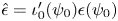 $\hat {\epsilon } = \iota _0'(\psi _0)\epsilon (\psi _0)$.
The fixed points of the magnetic field line flow in the  $(\psi _1, \varTheta )$ coordinates, which represent closed magnetic field lines, occur at
  $\textrm {d}\varTheta / \textrm {d}\varphi = \textrm {d}\psi _1 / \textrm {d}\varphi = 0$. This corresponds to
  $(\psi _1, \varTheta ) = (\bar {\psi }_1, \bar {\varTheta })$, such that
 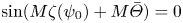 $\sin ( M \zeta (\psi _0) + M \bar {\varTheta } ) = 0$ and
  $\bar {\psi }_1 = \pm \epsilon '(\psi _0)/ \iota _0'(\psi _0) = O(\epsilon )$, where we have used
  $\cos ( M \zeta (\psi _0) + M \bar {\varTheta } ) = \mp 1$. Introducing magnetic coordinates relative to a closed magnetic field line,
  $\delta \psi = \psi - \psi _0 - \bar {\psi }_1$ and
  $\delta \varTheta = \varTheta - \bar {\varTheta }$, (2.14) and (2.15) linearized near the closed magnetic field give
 \begin{align} \frac{\textrm{d}}{\textrm{d}\varphi} \begin{pmatrix} \delta \psi \\ \delta \varTheta \end{pmatrix} = \begin{pmatrix} O(\hat{\epsilon}) & \mp \epsilon(\psi_0) M^2 + O(\epsilon \hat{\psi}_1) \\ \iota_0'(\psi_0) + O(\iota_0'(\psi_0)\hat{\epsilon} ) & O(\hat{\epsilon}) \end{pmatrix} \begin{pmatrix} \delta \psi \\ \delta \varTheta \end{pmatrix} . \end{align}
As will be shown explicitly by expanding the Hamiltonian near the closed field line, the error terms in (2.16), which arise from the diagonal elements of the matrix, are negligible because the only self-consistent ordering relating the characteristic sizes of  $\delta \psi$ and
  $\delta \varTheta$ is
  $|\iota _0'| \delta \psi \sim M \sqrt {\hat {\epsilon }} \delta \varTheta$. Trajectories neighbouring the island centre (O point) are described when the signs of the off-diagonal elements in the matrix in (2.16) are opposite, because in this case, the eigenvalues are purely imaginary and the trajectories are periodic. The other sign choice corresponds to the trajectories passing close to the crossing point of the island separatrices (X point). Thus, we can replace
  $\pm$ everywhere with
 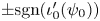 $\pm \text {sgn} ( \iota '_0 (\psi _0) )$, with the top and bottom signs understood to correspond to O and X points, respectively. The motion sufficiently close to the centre is thus always described by
 \begin{equation} \frac{\textrm{d}}{\textrm{d}\varphi} \begin{pmatrix} \delta \psi \\ \delta \varTheta \end{pmatrix} = \begin{pmatrix} O(\hat{\epsilon}) & - \text{sgn} \left( \iota'_0 (\psi_0) \right) \epsilon(\psi_0) M^2 ( 1 + O( \hat{\epsilon} )) \\ \iota_0'(\psi_0) (1 + O(\hat{\epsilon})) & O(\hat{\epsilon}) \end{pmatrix} \begin{pmatrix} \delta \psi \\ \delta \varTheta \end{pmatrix} , \end{equation}
where we have set  $\cos ( M \zeta (\psi _0) + M \bar {\varTheta } ) =- \text {sgn} ( \iota '_0 (\psi _0) )$ at an O point. Solving this linear system gives
 \begin{equation} \begin{pmatrix} \delta \psi (\varphi)\\ \delta \varTheta (\varphi) \end{pmatrix} = \textsf {T} \begin{pmatrix} \delta \psi(0) \\ \delta \varTheta(0) \end{pmatrix} {,} \end{equation}
where the tangent map  $\textsf {T}$ is given by
 \begin{equation} \textsf {T} \simeq \begin{pmatrix} \cos(\omega \varphi ) & - \left( \omega / \iota_0'(\psi_0) \right) \sin (\omega \varphi ) \\ \left( \iota_0'(\psi_0) / \omega \right) \sin (\omega \varphi ) & \cos(\omega \varphi ) \end{pmatrix} {,} \end{equation}
and the frequency at which neighbouring points rotate around the  $O$ point is
 \begin{equation} \omega \simeq M \sqrt{|\iota'_0(\psi_0)| \epsilon(\psi_0)} . \end{equation}
Note that, from (2.17), each element of the tangent map in (2.19) has an error of  $O(\hat {\epsilon })$ and the frequency
  $\omega$ in (2.20) has an error of
  $O( \hat {\epsilon } \sqrt {|\iota '_0(\psi _0)| \epsilon (\psi _0)} )$ (Cary & Hanson Reference Cary and Hanson1991).
To relate the linearized motion along a field line neighbouring the island centre, described by (2.18)–(2.20), to the island width, the motion along the island separatrix is studied. The Hamiltonian on the separatrix is constant and equal to its value at the  $X$ point,
 \begin{equation} K (\bar{\psi}, \bar{\varTheta} ) = \chi_0 ( \psi ) - \iota_0 ( \psi ) \psi_0 + \textrm{sgn} \left( \iota_0'(\psi_0) \right) \epsilon(\psi_0) + O(\hat{\epsilon}\epsilon) , \end{equation}
where we inserted  $\bar {\psi } = - \epsilon '(\psi _0)/ |\iota _0'(\psi _0)|$ (X point),
  $\sin ( M \zeta (\psi _0) + M \bar {\varTheta } ) = 0$ (fixed point) and
  $\cos ( M \zeta (\psi _0) + M \bar {\varTheta } ) = \text {sgn} ( \iota _0'(\psi _0) )$ (X point) in (2.13). From (2.13) and
  $\epsilon (\psi _0) > 0$, the value of
  $\psi _1^2$ is largest when
  $\cos ( M \zeta (\psi _0) + M \varTheta ) = -\text {sgn} ( \iota _0'(\psi _0) )$ on the separatrix, and so by evaluating
  $K (\psi , \varTheta )$ at this point and equating it to (2.21), we obtain
 \begin{equation} \tfrac{1}{2} | \iota_0'(\psi_0) | \psi_1^2 = 2 \epsilon(\psi_0) + O(\epsilon \hat{\psi}_1, \hat{\epsilon}\epsilon ) . \end{equation}
Hence, the values of  $\psi _1$ at the separatrix at the point where the island is largest are
  $\psi _1 = \pm 2 \sqrt { \epsilon (\psi _0) / | \iota _0'(\psi _0) | } + O(\epsilon ) \sim \sqrt {\hat {\epsilon }} / \iota _0'(\psi _0)$ and the full island width, denoted
  $\varUpsilon$, is
 \begin{equation} \varUpsilon = 4 \sqrt{ \frac{ \epsilon(\psi_0) }{\left| \iota_0'(\psi_0) \right| } }. \end{equation}
Note that  $\varUpsilon$ is approximately equal to the full island width in the magnetic coordinate
  $\psi$ with an absolute error of
  $O(\epsilon )$, equivalent to a relative error of
  $O( \hat {\epsilon }^{1/2})$. Note also that
  $|\bar {\psi } | \ll \varUpsilon$ and so the island centre is equidistant from the two branches of the separatrix to the lowest order in
  $\hat {\epsilon }$. From (2.20) and (2.23), the matrix
  $\textsf {T}$ in (2.19) can be rewritten with
  $\varUpsilon$ in place of
  $\iota _0'$ to obtain
 \begin{equation} \textsf {T} \simeq \begin{pmatrix} \cos(\omega \varphi ) & - \text{sgn} \left( \iota_0'(\psi_0) \right) \left( M \varUpsilon / 4 \right) \sin (\omega \varphi ) \\ \text{sgn} \left( \iota_0'(\psi_0) \right) \left( 4 / M \varUpsilon \right) \sin (\omega \varphi ) & \cos(\omega \varphi ) \end{pmatrix} {.} \end{equation}
 When linearizing the equations for the magnetic field line near the island centre, the associated Hamiltonian is (2.10) expanded near the island centre up to quadratic terms in  $\delta \psi$ and
  $\delta \varTheta$. Retaining only the lowest-order terms in
  $\epsilon$ gives
 \begin{align} K &= \text{const} + \tfrac{1}{2} \iota_0'(\psi_0) \delta \psi^2 + \tfrac{1}{2} \text{sgn} \left( \iota_0' (\psi_0) \right) M^2\epsilon \delta \varTheta^2 \nonumber\\ &\quad + O ( \hat{\epsilon} \delta \psi^2 \iota_0'(\psi_0 ), M^2 \hat{\epsilon} \delta \psi \delta \varTheta, M^2\hat{\epsilon} \epsilon \delta \varTheta , M^2\hat{\epsilon} \epsilon \delta \varTheta^2 ) , \end{align}
where we have deduced that the only self-consistent ordering is  $\iota _0'(\psi _0) \delta \psi \sim M \sqrt {\hat {\epsilon }} \delta \varTheta$. Note that (2.25) can be made to be exactly quadratic: the linear term in the error in (2.25) could be cancelled by calculating the first-order correction in
  $\hat {\epsilon }$ of the value of
  $\varTheta$ at the island centre and redefining
  $\delta \varTheta$ relative to this more accurate coordinate. The neglected
  $O(M^2 \hat {\epsilon } \delta \psi \delta \varTheta )$ cross-term in (2.25) gives rise to the diagonal terms in the matrix in (2.16), which have a negligible contribution once the ordering
  $\iota _0'(\psi _0) \delta \psi \sim M \sqrt {\hat {\epsilon }} \delta \varTheta$ is taken into account. The magnitude of the quadratic perturbation to the Hamiltonian,
 \begin{align} |\delta K | = \delta \boldsymbol{u} \boldsymbol{\cdot} \textsf {K} \boldsymbol{\cdot} \delta \boldsymbol{u} = \begin{pmatrix} \delta \psi , & \delta \varTheta \end{pmatrix} \begin{pmatrix} \frac{1}{2} | \iota_0'(\psi_0) | + O ( \hat{\epsilon} \iota_0'(\psi_0) ) & O(M^2\hat{\epsilon} ) \\ O(M^2\hat{\epsilon} ) & \frac{1}{2} M^2\epsilon + O (M^2\hat{\epsilon} \epsilon ) \end{pmatrix} \begin{pmatrix} \delta \psi \\ \delta \varTheta \end{pmatrix} {,} \end{align}
is a scalar invariant, as it is conserved following the field lines neighbouring the O point. To the lowest order in  $\hat {\epsilon }$,
  $\textsf {K}$ is diagonal and thus the trajectories infinitesimally close to the island centre in magnetic coordinates are ellipses that are approximately aligned with the magnetic coordinate directions and elongated in the
  $\varTheta$ direction. The angle between the characteristic directions of the ellipses and the magnetic coordinate axes is small,
  $O(\hat {\epsilon })$. Note that if we diagonalized the matrix
  $\textsf {K}$ exactly, we would obtain additional error terms of the same order in the diagonal terms.
2.2. Relating magnetic coordinates to lengths at the island centre
The relationship between the displacement from the island centre, measured as a length in the poloidal cross-section at a given  $\varphi$, and the same displacement, measured in magnetic coordinates, must be linear if the displacement is infinitesimal (as the relationship between the two sets of coordinates must be locally described by a Taylor expansion). Thus, we define the local linear change of variables
  $\delta \boldsymbol {u} = (\delta \psi , \delta \varTheta ) \rightarrow \delta \boldsymbol {\xi } = ( \delta \xi _{\perp }, \delta \xi _{\parallel } )$, where
  $\delta \xi _{\perp } (\varphi )$ and
  $\delta \xi _{\parallel }(\varphi )$ are displacements from the island centre in two orthogonal directions (yet unspecified) in the poloidal plane with toroidal angle
  $\varphi$. The two sets of coordinates are related by
  $\delta \boldsymbol {u} (\varphi ) = \textsf {Q} (\varphi ) \boldsymbol {\cdot } \delta \boldsymbol {\xi } (\varphi )$ for any
  $\varphi$, where
 \begin{equation} \textsf {Q}(\varphi ) = \begin{pmatrix} \dfrac{\partial \psi }{\partial \xi_{{\perp}}}(\varphi ) & \dfrac{\partial \psi }{\partial \xi_{{\parallel}}}(\varphi )\\ \dfrac{\partial \varTheta }{\partial \xi_{{\perp}}}(\varphi ) & \dfrac{\partial \varTheta }{\partial \xi_{{\parallel}}}(\varphi ) \end{pmatrix} . \end{equation}
For each value of  $\varphi$, the scalar invariant can be cast in the new coordinates,
  $|\delta K | = \delta \boldsymbol {\xi } (\varphi ) \boldsymbol {\cdot } \textsf {Q}^\intercal (\varphi )\boldsymbol {\cdot } \textsf {K} \boldsymbol {\cdot } \textsf {Q}(\varphi ) \boldsymbol {\cdot } \delta \boldsymbol {\xi } (\varphi )$, where
  $\textsf {Q}^{\intercal }$ denotes the transpose of
  $\textsf {Q}$ and the local laboratory invariant matrix
  $\textsf {Q}^\intercal (\varphi ) \boldsymbol {\cdot } \textsf {K} \boldsymbol {\cdot } \textsf {Q} (\varphi )$ is symmetric because
  $\textsf {K}$ is symmetric. Thus, the eigenvectors of the local laboratory invariant matrix are orthogonal and the points of intersection of a trajectory, infinitesimally close to the island centre, with any given poloidal plane
  $\varphi$ lie on an ellipse.
The dependence of the scalar invariant on  $\varphi$ expresses the fact that, when viewing the motion continuously in different
  $\varphi$-planes, the poloidal displacement of a field line infinitesimally close to the island centre lies on a continuously varying ellipse. This is a consequence of the fact that in a stellarator, the poloidal cross-section of flux surfaces taken at different toroidal angles is generally different, and thus the shape of the island continuously changes and rotates poloidally as the island centre is followed around. Nonetheless, a set of equivalent flux surface sections always exists for values of
  $\varphi$ that differ by an integer multiple of a field period,
  $2{\rm \pi} / n_0$, where
  $n_0 \geqslant 1$. The flux surface sections are, in general, only equivalent to the lowest order in the island-producing perturbation,
  $\epsilon$, because an island chain may break the field periodicity (
 $n_0 = 1$ is a special case where the field periodicity is never broken). The closed field line intersects the set of approximately equivalent poloidal planes a finite number of times,
  $L$, before returning to the original position. Therefore, when snapshots of the position along a field line neighbouring the island centre are taken at
  $\varphi = \varphi _k + 2{\rm \pi} Q L / n_0$ for any positive integer
  $Q$ and initial toroidal angle
  $\varphi _k$, the motion appears to be around the same ellipse. In this work, we choose one set of an infinite number of possible sets of symmetry planes by specifying the toroidal plane corresponding to
  $\varphi = 0$ and considering the set of symmetry planes given by
 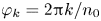 $\varphi _ k = 2{\rm \pi} k / n_0$, where
  $k$ is a positive integer. For stellarators with stellarator symmetry, the magnetic configuration in the plane
  $\varphi = 0$ is chosen to be up–down symmetric. Henceforth, any quantity that is a function of
  $\varphi _k$ will be denoted with a subscript
  $k$, e.g.
  $\textsf {Q}_k = \textsf {Q} (\varphi _k )$.
As the matrix  $\textsf {K}$ is (approximately) diagonal, the diagonalization of the invariant matrix
  $\textsf {Q}_k^\intercal \boldsymbol {\cdot } \textsf {K} \boldsymbol {\cdot } \textsf {Q}_k$ is achieved (approximately) by choosing the coordinates
  $\delta \xi _{\parallel , k}$ and
  $\delta \xi _{\perp , k}$ such that
  $\partial \psi / \partial \xi _{\parallel , k} = \partial \varTheta / \partial \xi _{\perp , k} = 0$ for all
  $k$ and thus
 \begin{gather} \delta \psi_k = \frac{\partial \psi}{\partial \xi_{{\perp},k}} \delta \xi_{{\perp}, k} , \end{gather}
 \begin{gather} \delta \varTheta_k = \frac{\partial \varTheta}{\partial \xi_{{\parallel}, k}} \delta \xi_{{\parallel}, k} . \end{gather}
With this choice, the coordinates  $\delta \xi _{\perp , k}$ and
  $\delta \xi _{\parallel , k}$ quantify the displacement (as a length) from the island centre in the poloidal plane
  $\varphi = 2{\rm \pi} k / n_0$, measured in the directions associated with
  $\delta \psi$ (across the flux surface) and
  $\delta \varTheta$ (along the flux surface), respectively. In the new coordinates, the displacement from the fixed point satisfies the equation
 \begin{equation} \delta \boldsymbol{\xi}_{k+q} (\varphi) = \textsf {S}_{R,k}^q \boldsymbol{\cdot} \delta \boldsymbol{\xi}_k , \end{equation}
where the tangent map in the rotating frame,  $\textsf {S}_{R,k}^q = \textsf {Q}_{k+q}^{-1} \boldsymbol {\cdot } \textsf {T}_{k+q} \boldsymbol {\cdot } \textsf {Q}_k$, is given by
 \begin{equation} \textsf {S}_{R,k}^q \simeq \begin{pmatrix} \dfrac{ \partial \xi_{{\perp}, k+q} }{ \partial \psi } \dfrac{ \partial \psi }{ \partial \xi_{{\perp}, k} } \cos\left( \dfrac{2{\rm \pi} \omega q }{ n_0} \right) & - \dfrac{ \partial \xi_{{\perp}, k+q} }{ \partial \psi } \dfrac{ \partial \varTheta }{ \partial \xi_{{\parallel}, k} } \dfrac{ M\varUpsilon }{ 4} \sin\left( \dfrac{2{\rm \pi} \omega q }{ n_0} \right)\\ \dfrac{ \partial \xi_{{\parallel}, k+q} }{ \partial \varTheta } \dfrac{ \partial \psi }{ \partial \xi_{{\perp}, k} } \dfrac{ 4}{ M\varUpsilon } \sin \left( \dfrac{2{\rm \pi} \omega q }{ n_0} \right) & \dfrac{ \partial \xi_{{\parallel}, k+q} }{ \partial \varTheta } \dfrac{ \partial \varTheta }{ \partial \xi_{{\parallel}, k} } \cos\left( \dfrac{2{\rm \pi} \omega q }{ n_0} \right) \end{pmatrix} {.} \end{equation}
Note that
 \begin{equation} \bar{w}_{{\perp}, k} = \varUpsilon \frac{ \partial \xi_{{\perp}, k} }{ \partial \psi } \end{equation}
is approximately equal to the island width measured at  $\varphi = 2{\rm \pi} k / n_0$, with an absolute error of
  $O( \varUpsilon ^2 \partial ^2 \xi _{\perp , k} / \partial \psi ^2 )$, which gives rise to a relative error of
  $O(\hat {\epsilon }^{1/2} )$. This relative error is to be added to the equally large error in approximating the island width in the coordinate
  $\psi$ as
  $\varUpsilon$ in (2.23). Using (2.32), the off-diagonal elements of
  $\textsf {S}_{R,k}^q$ explicitly include the island width. Upon imposing
  $\delta \xi _{\parallel , k} = 0$ as an initial condition, we obtain the equation
 \begin{equation} \frac{\delta \xi_{{\parallel}, k+q} }{ \delta \xi_{{\perp}, k}} \simeq \frac{ \partial \xi_{{\parallel}, k+q} }{ \partial \varTheta } \frac{4}{ M \bar{w}_{{\perp}, k} } \sin \left( \frac{2{\rm \pi} \omega q}{n_0} \right) {,} \end{equation}
where only the bottom-left element of (2.31) appears.
Because the derivative in  $\partial \xi _{\parallel , k+q} / \partial \varTheta$ is taken at fixed
  $\varphi$, the definition of
  $\varTheta$ in (2.8) implies that
 \begin{equation} \frac{\partial \xi_{{\parallel}, k+q}}{\partial \theta} = \frac{\partial \xi_{{\parallel}, k+q}}{\partial \varTheta} . \end{equation}
Integrating in  $\theta$ at fixed
  $\varphi = \varphi _{k+q}$ gives the circumference
  $\bar C$ around the unperturbed flux surface,
 \begin{equation} \bar C = \int_{-{\rm \pi}}^{\rm \pi} \frac{\partial \xi_{{\parallel}, k+q}}{\partial \theta} \,\textrm{d}\theta . \end{equation}
Because each plane under consideration, given by  $\varphi = 2{\rm \pi} ( k + q) / n_0$, has the same unperturbed flux surface independent of the value of
  $k+q$, the circumference is independent of the index and thus
  $\bar C = \bar C_{k+q}$. Consider the definition of
  $\varTheta$ in (2.8). Following the island centre,
  $\varTheta _{k+q} = \varTheta _k = \theta _k - N \varphi _k / M$ is conserved and therefore the poloidal angle changes according to the equation
  $\theta _{k+q} - \theta _k = 2{\rm \pi} Nq / (n_0 M)$. Because we are only considering the set of equivalent planes separated by intervals of
  $2{\rm \pi} / n_0$ in
  $\varphi$, the poloidal angles
  $\theta _{k+q}$ correspond to the same flux surface poloidal cross-section. The field line first returns to the same poloidal location in an equivalent plane when
  $N L / (n_0 M) = \bar {n}$, where
  $L$ and
  $\bar {n}$ are the smallest possible integers that satisfy this relation. Thus, the number of distinct islands crossed by a unique island centre magnetic field line in an equivalent poloidal plane is
 \begin{equation} L = \frac{\bar{n} n_0}{N} M \rm . \end{equation}
The interval in poloidal angle  $\theta$, when defined from
  $-{\rm \pi}$ to
  ${\rm \pi}$, between the fixed points in a given plane is
  $2{\rm \pi} / L$, as there are
  $L$ equally-spaced fixed points. Thus, if
  $L$ is sufficiently large,
  $L \gg 1$, the integral in (2.35) can be replaced by a sum, and the circumference can be approximated by
 \begin{equation} \bar C \simeq \frac{2{\rm \pi}}{L} \sum_{q=q_0 }^{q_0+L-1} \frac{\partial \xi_{{\parallel}, k+q}}{\partial \theta} \simeq \sum_{q=q_0}^{q_0 + L-1} \frac{ {\rm \pi}( \delta \xi_{{\parallel}, k+q } / \delta \xi_{{\perp}, k} ) M \bar{w}_{{\perp}, k} }{2L \sin \left( 2{\rm \pi} \omega q / n_0 \ \right) } . \end{equation}
The error made in approximating the integral over the periodic function  $\theta$ as a sum with equally-spaced integration points is exponentially small in
  $1/L$,
  $O( \exp (-L) )$.
The integer  $q_0$ can be chosen arbitrarily, although a convenient choice is made as follows. If
  $\sin ( 2{\rm \pi} \omega (k+q) / n_0 ) = 0$, the denominator in the summand with index
  $q$ is zero. However, no matter how precise, a numerical calculation of
  $\delta \xi _{\parallel , k+q}$ will not give exactly zero, owing to the fact that the elliptical motion described using the tangent map (2.24) has small errors both in the aspect ratio and in the axes directions (the higher-order terms in
  $\hat {\epsilon }$ that were neglected). To avoid the resulting divergence of the error, the first index of the summand is chosen such that the the sum is centred around
  $\sin ( 2{\rm \pi} \omega q / n_0 ) = 1$,
  $2{\rm \pi} \omega (q_0 + L/2 ) / n_0 = {\rm \pi}/ 2$, which gives
 \begin{equation} q_0 = \text{int}\left( - \frac{L}{2} + \frac{n_0 }{ 4 \omega } \right) , \end{equation}
where int denotes a function that rounds to the nearest integer. This amounts to following the linearized trajectory for a large number,  $q_0 / L$, of closed magnetic field line periods. With this choice, the linearized trajectory is followed until it has rotated by as close as possible to
  ${\rm \pi} / 2$ in magnetic coordinates for values of
  $q$ in the middle of the summation interval. Moreover, we assume that the frequency of rotation,
  $\omega$ in (2.20), is sufficiently small that the change in the quantity
  $2{\rm \pi} \omega (k+q) / n_0$ in the summation interval
  $q_0 \leqslant q < q_0 + L$ is also small,
  $2{\rm \pi} \omega L / n_0 \ll 1$, which gives
  $\sin ( 2{\rm \pi} \omega q / n_0 ) \simeq 1$ for all values of
  $q$ in the sum and thus
 \begin{equation} C \simeq \frac{M{\rm \pi}}{2L} \sum_{q=q_0}^{q_0 + L-1} \frac{ \delta \xi_{{\parallel}, k+q } }{ \delta \xi_{{\perp}, k} } \bar{w}_{{\perp}, k} . \end{equation}
In Cary & Hanson (Reference Cary and Hanson1991), this assumption is not made and the sine function in (2.37) is kept. Using (2.20) and the pessimistic ordering in which  $L/n_0$ is largest,
  $L \sim n_0 M$, this assumption requires the modestly stricter ordering
  $2{\rm \pi} M^2 \sqrt {\iota '_0 \epsilon } \sim 2{\rm \pi} M^2 \sqrt {\hat {\epsilon }} \ll 1$.Footnote 1
2.3. Cylindrical coordinates
Because stellarators are toroidal devices, we choose the right-handed cylindrical coordinates  $(R, \varphi , Z)$ as a convenient fixed coordinate system. Here,
  $\varphi$ is the toroidal coordinate,
  $R$ is the smallest distance of a point from the axis through the centre of the torus and
  $Z$ is the displacement of a point from the mid-plane of the device.
In the following, we study the equations describing the magnetic field line poloidal position,  $\boldsymbol {X} = (R, Z)$, as a function of toroidal angle
  $\varphi$. Considering the magnetic field line as a streamline of the flow field
  $\boldsymbol {B}$, the streamline trajectory satisfies
 \begin{equation} \frac{R\textrm{d}\varphi}{B_{\varphi}} = \frac{\textrm{d}R}{B_R} = \frac{\textrm{d}Z}{B_Z} , \end{equation}
and thus
 \begin{equation} \frac{\textrm{d}\boldsymbol{X}}{\textrm{d}\varphi} = \boldsymbol{V}(\boldsymbol{X}, \varphi) \equiv \frac{R \boldsymbol{B}_p (\boldsymbol{X} , \varphi )}{ B_{\varphi}(\boldsymbol{X}, \varphi)} , \end{equation}
where we have denoted the component of the magnetic field vector in the poloidal plane as  $\boldsymbol {B}_{p} = (B_R, B_Z)$. To obtain the position of a magnetic field line at
  $\varphi = \varphi _{k+q}$, we integrate (2.41) in
  $\varphi$ from an initial poloidal position
  $\boldsymbol {X}_k = \boldsymbol {X} ( \varphi _k )$,
 \begin{equation} \boldsymbol{X}_{k+q} = F^q_k \left( \boldsymbol{X}_{k} \right) \equiv \boldsymbol{X}_k + \int_{\varphi_k}^{\varphi_{k+q}} \boldsymbol{V}(\boldsymbol{X}(\varphi), \varphi) \,\textrm{d}\varphi . \end{equation}
A closed magnetic field line  $\bar {\boldsymbol {X}}$, such as the island centre, satisfies
 \begin{equation} \bar{\boldsymbol{X}}_{k+L} = F^L_k (\boldsymbol{X}_k) = \bar{\boldsymbol{X}}_k {.} \end{equation}
 For an initial condition that is infinitesimally close to the island centre,  $\boldsymbol {X}(\varphi _k ) = \bar {\boldsymbol {X}}_{k} + \delta \boldsymbol {X} (\varphi _k)$, the displacement from the closed field line as a function of toroidal angle satisfies the linearized equation
 \begin{equation} \frac{\textrm{d}\delta \boldsymbol{X}}{\textrm{d}\varphi} = \left[ \boldsymbol{\nabla}_{\boldsymbol X} \boldsymbol{V} \left( \bar{\boldsymbol{X}}, \varphi \right) \right]^{\intercal} \boldsymbol{\cdot} \delta \boldsymbol{X} , \end{equation}
where the Jacobian of the field-line-following equation is
 \begin{equation} \boldsymbol{\nabla}_{\boldsymbol X} \boldsymbol{V} = \frac{ \hat{\boldsymbol{e}}_R \boldsymbol{B}_p (\bar{\boldsymbol{X}} , \varphi )}{ B_{\varphi}(\bar{\boldsymbol{X}}, \varphi)} + \frac{R \boldsymbol{\nabla}_{\boldsymbol X} \boldsymbol{B}_p (\bar{\boldsymbol{X}} , \varphi )}{ B_{\varphi}(\bar{\boldsymbol{X}}, \varphi)} - \frac{R ( \boldsymbol{\nabla}_{\boldsymbol X} B_{\varphi}(\bar{\boldsymbol{X}}, \varphi) ) \boldsymbol{B}_p (\bar{\boldsymbol{X}} , \varphi ) }{ B_{\varphi}(\bar{\boldsymbol{X}}, \varphi)^2} . \end{equation}
We have denoted  $[ \boldsymbol {\nabla }_{\boldsymbol X} \boldsymbol {V} ]^{\intercal } \boldsymbol {\cdot } \delta \bar {\boldsymbol {X}} = \delta \bar {R} \partial \boldsymbol {V} / \partial R + \delta \bar {Z} \partial \boldsymbol {V} / \partial Z$, and
  $\hat {\boldsymbol {e}}_R = \boldsymbol {\nabla }_{\boldsymbol X} R$. It is useful to introduce a
  $2\times 2$ matrix
  $\textsf {S}_k(\varphi )$ that solves a similar equation to (2.44),
 \begin{equation} \frac{\textrm{d} \textsf {S}_k }{\textrm{d}\varphi} = \left[ \boldsymbol{\nabla}_{\boldsymbol X} \boldsymbol{V} \left( \bar{\boldsymbol{X}}, \varphi \right) \right]^{\intercal} \boldsymbol{\cdot} \textsf {S}_k (\varphi) , \end{equation}
with initial condition  $\textsf {S}_k(\varphi _k) = \textsf {I}$. Then, any solution to (2.44) can be found from
  $\delta \boldsymbol {X}(\varphi ) = \textsf {S}_k(\varphi ) \delta \boldsymbol {X}(\varphi _k)$, as can be verified by substituting this expression into (2.44). Denoting
  $\textsf {S}_k(\varphi _{k+q}) = \textsf {S}_k^q$ gives the equation
 \begin{equation} \delta \boldsymbol{X}_{k+q} = \textsf {S}_k^q \delta \boldsymbol{X}_k {,} \end{equation}
so we can identify  $\textsf {S}_k^q$ with
  $\textsf {S}_{R,k}^q$ in (2.30)–(2.31). The tangent map
  $\textsf {S}_k^q$ is obtained from the integral
 \begin{equation} \textsf {S}_k^q \equiv \textsf {I} + \int_{\varphi_k}^{\varphi_{k+q}} \left[ \boldsymbol{\nabla}_{\boldsymbol X} \boldsymbol{V} \left( \bar{\boldsymbol{X}}, \varphi \right) \right]^{\intercal} \boldsymbol{\cdot} \textsf {S}_k (\varphi) \,\textrm{d}\varphi {.} \end{equation}
To carry out this integration, the function  $\bar {\boldsymbol {X}}(\varphi )$ must be calculated separately from (2.41). As the tangent map is linear in
  $\delta \boldsymbol {X}$, it satisfies the property
 \begin{equation} \textsf {S}_k^q \equiv \textsf {S}^1_{k+q-1} \textsf {S}_{k+q-2}^1 \ldots \textsf {S}_{k+1}^1 \textsf {S}_{k}^1 . \end{equation}
The full-orbit tangent map is denoted as
 \begin{equation} \textsf {M}_k = \textsf {S}_k^{L} {.} \end{equation}
An important property of the full-orbit tangent map is that it has exactly unit determinant,  $\det (\textsf {M}_k ) = 1$ for all
  $k$ (Cary & Hanson Reference Cary and Hanson1986). This follows from the underlying Hamiltonian nature of the magnetic field line trajectory (Meiss Reference Meiss1992). Thus, the characteristic equation for the eigenvalues of
  $\textsf {M}_k$ is
  $\lambda ^2 - \lambda \text {Tr} ( \textsf {M}_k ) + 1 = 0$, which gives
 \begin{equation} \lambda = \tfrac{1}{2} \text{Tr} ( \textsf {M}_k ) \pm \sqrt{ \left( \tfrac{1}{2} \text{Tr} ( \textsf {M}_k ) \right)^2 - 1 } {.} \end{equation}
Hence, for  $| \text {Tr} ( \textsf {M}_k ) | < 2$, the eigenvalues are complex numbers on the unit circle,
  $\lambda _{\pm } = \exp ( \pm i \alpha )$, with
 \begin{equation} \alpha = \arccos \left( \tfrac{1}{2} \text{Tr} (\textsf {M}_k ) \right) {.} \end{equation}
The angle  $\alpha$ is the average angle of rotation around the island centre of a neighbouring trajectory after the island centre returns to its original poloidal position. For this reason, it takes the same value irrespective of the fixed point
  $k$ used to calculate it. From (2.19), the average angle of rotation after following around the island centre is
  $2{\rm \pi} \omega L / n_0$. Hence, we obtain an expression for the average frequency of rotation of linearized trajectories about the island centre,
 \begin{equation} \omega = \frac{n_0}{2{\rm \pi} L} \arccos \left( \frac{1}{2} \text{Tr} (\textsf {M}_k ) \right) {.} \end{equation}
 It is useful to recall that a closed magnetic field line is not necessarily an island centre. Because the relation  $\det (\textsf {M}_k) = 1$ always holds, the closed field line can be elliptic or hyperbolic: it can be an O point or an X point, respectively. When the closed field line is not an O point, the concept of a rotation frequency breaks down. A quantity that can be used to determine whether the closed field line is a centre or an X point is the residue (Greene Reference Greene1968) of the full-orbit tangent map,
 \begin{equation} \mathcal{R} = \tfrac{1}{2} - \tfrac{1}{4} \text{Tr} (\textsf {M}_k ) . \end{equation}
For  $0 < \mathcal {R} < 1$, a rotation frequency can be calculated from (2.53) and thus the closed field line is a centre. If
  $\mathcal {R} < 0$ or
  $\mathcal {R} > 1$, the closed field line is an X point, as the magnitude of the trace is greater than unity and (2.53) does not have a real solution for
  $\omega$. In the island width calculation of this section, it is not only assumed that
  $0 < \mathcal {R} < 1$, but also that
  $\mathcal {R} \ll 1$ such that
  $2{\rm \pi} \omega L / n_0 \ll 1$.
Two-dimensional matrices with unit determinant, such as  $\textsf {M}_k$, satisfy the equation
 \begin{equation} \textsf {M}_k^{\mathrm{T}} \boldsymbol{\sigma} \textsf {M}_k = \textsf {M}_k \boldsymbol{\sigma} \textsf {M}_k^{\mathrm{T}} = \boldsymbol{\sigma} , \end{equation}
with
 \begin{equation} \sigma = \begin{pmatrix} 0 & 1 \\ -1 & 0 \end{pmatrix} {.} \end{equation}
From (2.55), we get  $\textsf {M}_k^{\mathrm {T}} ( \boldsymbol {\sigma } \textsf {M}_k ) \textsf {M}_k = \boldsymbol {\sigma } \textsf {M}_k$. Therefore, the matrix
  $\boldsymbol {\sigma } \textsf {M}_k$ is an invariant of the full-orbit tangent map. The symmetrized matrix
 \begin{equation} \textsf {W}_k = \tfrac{1}{2} \left( \sigma \textsf {M}_k + \textsf {M}_k^\intercal \sigma^\intercal \right) \end{equation}
satisfies the same property that the unsymmetrized counterpart  $\boldsymbol {\sigma } \textsf {M}_k$ satisfies,
 \begin{equation} \textsf {M}_k^{\mathrm{T}} \boldsymbol{\cdot} \textsf {W}_k \boldsymbol{\cdot} \textsf {M}_k = \textsf {W}_k {.} \end{equation}
 Consider the scalar invariant discussed after (2.27) calculated at  $\varphi = \varphi _k$,
  $|\delta K | = \delta \boldsymbol {\xi }_k^\intercal \boldsymbol {\cdot } \textsf {Q}_k^\intercal \boldsymbol {\cdot } \textsf {K} \boldsymbol {\cdot } \textsf {Q}_k \boldsymbol {\cdot } \delta \boldsymbol {\xi }_k$. This quantity is constant on a trajectory that crosses the planes
  $\varphi = 2{\rm \pi} (k+LQ) / n_0$, where
  $Q$ is an integer, as it directly follows from the quadratic perturbation to the Hamiltonian (in the magnetic coordinate analysis) about the island centre,
  $|\delta K | = \delta \boldsymbol {u}^\intercal \boldsymbol {\cdot } \textsf {K} \boldsymbol {\cdot } \delta \boldsymbol {u}$. Similarly, the quantity
  $\delta \boldsymbol {X}_k^\intercal \boldsymbol {\cdot } \textsf {W}_k \boldsymbol {\cdot } \delta \boldsymbol {X}$ is constant on a trajectory that crosses the plane
  $\varphi = 2{\rm \pi} (k + LQ) / n_0$, because
  $\delta \boldsymbol {X}_k^\intercal \boldsymbol {\cdot } \textsf {M}_k^\intercal \boldsymbol {\cdot } \textsf {W}_k \boldsymbol {\cdot } \textsf {M}_k \boldsymbol {\cdot } \delta \boldsymbol {X}_k = \delta \boldsymbol {X}_k^\intercal \boldsymbol {\cdot } \textsf {W}_k \boldsymbol {\cdot } \delta \boldsymbol {X}_k$. The vectors
  $\delta \boldsymbol {X}_k$ and
  $\delta \boldsymbol {\xi }_k$ are equivalent displacement vectors expressed in two different coordinate systems that are rotated with respect to one another. Because the scalar invariant remains unchanged after a rotation, the two invariants can only be related by an overall constant,
  $\delta \boldsymbol {X}_k^\intercal \boldsymbol {\cdot } \textsf {W}_k \boldsymbol {\cdot } \delta \boldsymbol {X}_k = \gamma _k | \delta K |$ (Cary & Hanson Reference Cary and Hanson1991). Hence, the symmetric invariant matrix
  $\textsf {W}_k$ has the same unit eigenvectors as the (approximately diagonal) matrix
 \begin{align} \textsf {Q}_k^\intercal \boldsymbol{\cdot} \textsf {K} \boldsymbol{\cdot} \textsf {Q}_k = \begin{pmatrix} \dfrac{1}{2} \iota_0'(\psi_0) \left(\dfrac{\partial \psi}{ \partial \xi_{{\perp}} } \right)^2 + O \left( \dfrac{ \epsilon }{ \bar{C}^2} \right) & O \left( \dfrac{ M^2 \epsilon }{ \bar{C}^2} \right)\\ O \left( \dfrac{ M^2 \epsilon }{ \bar{C}^2} \right) & \dfrac{1}{2} M^2\epsilon \left(\dfrac{ \partial \xi_{{\parallel}} }{\partial \varTheta} \right)^2 + O \left( \dfrac{ M^2 \hat{\epsilon}\epsilon }{\bar{C}^2} \right) \end{pmatrix} , \end{align}
where, in the error terms, we have assumed that  $| \partial \boldsymbol {\xi } / \partial \varTheta | \sim \bar C$ and
 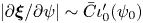 $| \partial \boldsymbol {\xi } / \partial \psi | \sim \bar C \iota '_0 (\psi _0)$. Moreover, the eigenvalues of
  $\textsf {W}_k$ are equal to the eigenvalues of
  $\textsf {Q}_k^\intercal \boldsymbol {\cdot } \textsf {K} \boldsymbol {\cdot } \textsf {Q}_k$ multiplied by a factor of
  $\gamma _k$. From (2.59), the smallest eigenvalue of
  $\textsf {Q}_k^\intercal \boldsymbol {\cdot } \textsf {K} \boldsymbol {\cdot } \textsf {Q}_k$ is approximately equal to the bottom-right element associated with the eigenvector
  $(\delta \xi _{\perp }, \delta \xi _{\parallel }) \simeq ( O(\hat {\epsilon }), 1+ O(\hat {\epsilon }))$, and the largest eigenvalue is approximately equal to the top-left element associated with the eigenvector
  $(\delta \xi _{\perp }, \delta \xi _{\parallel }) = ( 1 + O(\hat {\epsilon }), O(\hat {\epsilon }) )$. Therefore, the eigenvector of
  $\textsf {W}_k$ corresponding to the smallest eigenvalue is approximately tangent to the flux surface, and is denoted as
  $\hat {\boldsymbol {e}}_{k\parallel }$, and the eigenvector corresponding to the largest eigenvalue is approximately normal to the flux surface, and is denoted as
  $\hat {\boldsymbol {e}}_{k\perp }$. Because
  $\hat {\boldsymbol {e}}_{k\parallel }$ and
  $\hat {\boldsymbol {e}}_{k\perp }$ are simply defined as eigenvectors of
  $\textsf {W}_k$, their sign is yet unspecified. We impose the constraint
  $\hat {\boldsymbol {e}}_{\parallel , k} \boldsymbol {\cdot } \textsf {M}_k \boldsymbol {\cdot } \hat {\boldsymbol {e}}_{\perp , k} > 0$ for all
  $k$ to fix the relative sign of the eigenvectors.
2.4. Island width
An expression for the island width at  $\varphi = \varphi _k = 2{\rm \pi} k / n_0$ can be obtained by rearranging (2.39),
 \begin{equation} \bar{w}_{{\perp}, k} = \frac{2L\bar{C} }{M{\rm \pi} } \left( \sum_{q=q_0}^{q_0+L-1} \frac{ \delta \xi_{{\parallel}, k+q } }{ \delta \xi_{{\perp}, k} } \right)^{{-}1} . \end{equation}
Recall that  $\delta \xi _{\parallel , k} = 0$ and
  $q_0$ is chosen for convenience according to (2.38), such that
  $\delta \xi _{\perp , k+q} \simeq 0$ for all
  $q$ in the sum. An accurate calculation of the island width thus rests upon an accurate calculation of
  $\bar {C}$ and
 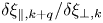 $\delta \xi _{\parallel , k+q } / \delta \xi _{\perp , k}$.
To calculate  $\delta \xi _{\parallel , k+q } / \delta \xi _{\perp , k}$, we follow the linearized magnetic field with initial condition
 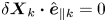 $\delta \boldsymbol {X}_k \boldsymbol {\cdot } \hat {\boldsymbol {e}}_{\parallel k} = 0$, which corresponds to
  $\delta \xi _{\parallel , k} \simeq 0$ and
 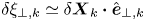 $\delta \xi _{\perp , k} \simeq \delta \boldsymbol {X}_k \boldsymbol {\cdot } \hat {\boldsymbol {e}}_{\perp , k}$. Using (2.46), or repeated application of partial tangent maps as in (2.49), we obtain
 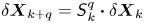 $\delta \boldsymbol {X}_{k+q} = \textsf {S}^q_k \boldsymbol {\cdot } \delta \boldsymbol {X}_k$. The final displacement from the fixed point in the direction parallel to the flux surface is
  $\delta \xi _{\parallel , k+q} \simeq \hat {\boldsymbol {e}}_{\parallel , k+q} \boldsymbol {\cdot } \delta \boldsymbol {X}_{k+q}$, which gives
 \begin{equation} \frac{ \delta \xi_{{\parallel}, k+q} }{\delta \xi_{{\perp}, k}} \simeq \hat{\boldsymbol{e}}_{{\parallel},k+q} \boldsymbol{\cdot} \textsf {S}_k^q \boldsymbol{\cdot} \hat{\boldsymbol{e}}_{{\perp}, k} . \end{equation}
Equation (2.61) is defined to be positive for all  $k$ and
  $q$, which provides a second constraint to fix the sign of the vectors
  $\hat {\boldsymbol {e}}_{\perp , k}$ and
  $\hat {\boldsymbol {e}}_{\parallel , k}$. With this additional constraint, the signs of the eigenvectors
  $\hat {\boldsymbol {e}}_{\perp ,k}$,
  $\hat {\boldsymbol {e}}_{\parallel ,k}$,
  $\hat {\boldsymbol {e}}_{\perp , k+q}$ and
  $\hat {\boldsymbol {e}}_{\parallel , k+q}$ for all
  $k$ and
  $q$ are specified with respect to one another. Note that the two constraints can only both be self-consistently applied if the small island width approximation is valid; if attempting to apply both constraints leads to a contradiction, the islands are too wide. We then have
 \begin{equation} \sum_{q=q_0}^{q_0+L-1} \frac{ \delta \xi_{{\parallel}, k+q } }{ \delta \xi_{{\perp}, k} } \simeq \varSigma_k \equiv \sum_{q=q_0}^{q_0+L-1} \hat{\boldsymbol{e}}_{{\parallel},k+q} \boldsymbol{\cdot} \textsf {S}_k^q \boldsymbol{\cdot} \hat{\boldsymbol{e}}_{{\perp}, k} {,} \end{equation}
where we have defined the positive quantity  $\varSigma _k$.
The circumference  $\bar {C}$ can be approximated, for a sufficiently large number of fixed points, from the sum of the chords in the poloidal plane. However, to obtain the appropriate chords, the fixed points must first be reordered to proceed monotonically around the flux surface. To do so, we consider a reordering function
  $\rho (k)$ such that
  $p = \rho (k)$ is the index labelling the reordered fixed points. We define
  $\rho (0) = 0$ such that
  $p=0$ for
  $k =0$, i.e. the set of reordered fixed points have the same point indexed as zero as the set of fixed points ordered by following the field line. Moreover, we reorder the fixed points to monotonically circulate the magnetic axis in the same direction that they appear to circulate when ordered following the magnetic field. The inverse of the reordering function is denoted as
  $\rho ^{-1}$ and is defined such that
  $\rho ^{-1}(\rho (k)) = k$, i.e. the field-line-following index
  $k$ is returned for a given reordered index
  $p$. It can be shown that
 \begin{equation} \rho(k) = (n_\textrm{turns} k)\ \text{mod}\ L \end{equation}
and
 \begin{equation} \rho^{{-}1}(p) = \frac{ \left(p\ \text{mod}\ n_{\text{turns}} \right)L + p }{n_{\text{turns}}} \text{ mod } L , \end{equation}
where  $n_\textrm {turns}$ is the total number of poloidal turns around the magnetic axis when following the field-line-ordered fixed points
  $\boldsymbol {X}_k$ (i.e. the number of times that the magnetic axis appears to have been circulated poloidally). Here,
  $k \text { mod } q$ indicates the remainder of
  $k/q$, equal to an integer between
  $0$ and
  $q-1$. The circumference
  $\bar C$ is approximated by the sum of the chords obtained by joining the reordered fixed points,
 \begin{equation} \bar C \simeq C \equiv \sum_{k=0}^{L-1} \left| \boldsymbol{c}_{k} \right| {,} \end{equation}
where
 \begin{equation} \boldsymbol{c}_{k} = \boldsymbol{X}_{k} - \boldsymbol{X}_{k_-} , \end{equation}
and  $\boldsymbol {X}_{k_-}$ is the fixed point preceding
  $\boldsymbol {X}_{k}$ in the reordered set, such that
 \begin{equation} k_-{=} \rho^{{-}1}(\rho(k) - 1) \rm . \end{equation}
The relative error in the chord approximation, i.e.  $\bar {C} \simeq C$, is
  $O(1/L)$.
Using (2.60), (2.62) and (2.65), the analytical small island width  $\bar {w}_{\perp , k}$ can be approximated by
  $\bar {w}_{\perp , k} \simeq w_{\perp , k}$, where
 \begin{equation} w_{{\perp}, k} \equiv \frac{2LC }{M{\rm \pi} \varSigma_k} . \end{equation}
The value of  $M$ is obtained by counting how many of the
  $L$ fixed points
  $\bar {\boldsymbol {X}}_k$ are also fixed points in the plane
  $\varphi = 0$, i.e.
  $\boldsymbol X (2{\rm \pi} L / n_0 ) = \boldsymbol X(0) = \bar {\boldsymbol {X}}_k$ is satisfied. The relative error in the island width
  $w_{\perp , k}$ compared with the true island width is
  $O(\hat {\epsilon }^{1/2}, L^{-1})$. The
  $O(\hat {\epsilon }^{1/2})$ part comes from the error in approximating the width in the coordinate
  $\psi$ using
  $\varUpsilon$ in (2.23) and the additional error in relating changes in
  $\psi$ to lengths in (2.32). The
  $O(L^{-1})$ part comes from the chord approximation. Considering instead the relative error between
  $w_{\perp , k}$ in (2.68) and
  $\bar {w}_{\perp , k}$ in (2.32), this is
  $O(\hat {\epsilon }, L^{-1})$. Here, the
  $O(\hat {\epsilon })$ part comes from the error in (2.61), which in turn comes from the
  $O(\hat {\epsilon })$ error in the bottom-left matrix element of (2.31) owing to the matrix
  $\textsf {K}$ in (2.26) only being approximately diagonal.
3. Island size and residue variation using adjoint equations
Here we consider the variation of the different quantities – including the width – related to magnetic islands following the infinitesimal variation of the magnetic field configuration from  $\boldsymbol {B} (\boldsymbol {R})$ to
  $\boldsymbol {B} (\boldsymbol {R}) + \Delta \boldsymbol {B} (\boldsymbol {R})$. From (2.68), the variation of the island width is
 \begin{equation} \frac{\Delta w_{{\perp},k}}{w_{{\perp},k}} \simeq \frac{ \Delta C }{C} - \frac{ \Delta \varSigma_k }{ \varSigma_k } {,} \end{equation}
where  $\Delta C$ is the variation of the circumference, approximated by the sum of chords in (2.65), and
  $\Delta \varSigma _k$ is the variation of the sum in (2.62). Most of this section is devoted to deriving expressions for
  $\Delta C$ and
  $\Delta \varSigma _k$, in terms of
  $\Delta \boldsymbol {B} ( \boldsymbol {R})$, using an adjoint method. In the final subsection, an expression for
  $\Delta \mathcal {R}$ is derived. Note that the variation of the on-axis rotational transform is directly related to
  $\Delta \mathcal {R}$ if one considers the magnetic axis as the periodic field line instead of an island chain O or X point.
3.1. Circumference variation
A result of the change in magnetic configuration from  $\boldsymbol {B} (\boldsymbol {R})$ to
  $\boldsymbol {B} (\boldsymbol {R}) + \Delta \boldsymbol {B} (\boldsymbol {R})$ is that the periodic field line position changes from
  $\bar {\boldsymbol {X}}(\varphi )$ to
  $\bar {\boldsymbol {X}}(\varphi ) + \Delta \bar {\boldsymbol {X}} ( \varphi )$. For the purpose of the island width calculation, the variation of the periodic field line position affects the circumference. This changes from
  $C$ in (2.65) to
  $C+ \Delta C$, where
  $\Delta C$ is given by
 \begin{equation} \Delta C(\bar{\boldsymbol{X}}(\varphi); \Delta \bar{\boldsymbol{X}}(\varphi)) = \sum_{k=1}^L \left( \Delta \bar{\boldsymbol{X}}_k - \Delta \bar{\boldsymbol{X}}_{k_-} \right) \boldsymbol{\cdot} \hat{\boldsymbol{c}}_k , \end{equation}
where  $\hat {\boldsymbol {c}}_{k} = \boldsymbol {c}_{k} / |\boldsymbol {c}_{k} |$. Equation (3.2) can be re-expressed as
 \begin{equation} \Delta C(\bar{\boldsymbol{X}}(\varphi); \Delta \bar{\boldsymbol{X}}(\varphi)) = \int_0^{2{\rm \pi} L/n_0} \,\textrm{d}\varphi \Delta \bar{\boldsymbol{X}} ( \varphi ) \boldsymbol{\cdot} \left[ \sum_{k=0}^{L-1} \hat{\boldsymbol{c}}_k ( \delta (\varphi - \varphi_k ) - \delta (\varphi - \varphi_{k_-}) ) \right] . \end{equation}
Notice that the second sum in (3.3) can be re-cast as
 \begin{equation} \sum_{k'=0}^{L-1} \hat{\boldsymbol{c}}_{k'} \delta (\varphi - \varphi_{k'_-}) = \sum_{k=0}^{L-1} \hat{\boldsymbol{c}}_{k_+} \delta (\varphi - \varphi_k ) , \end{equation}
where
 \begin{equation} k_+{=} \rho^{{-}1}(\rho(k)+1) , \end{equation}
because the order in which the sum is taken is not important. Re-expressing (3.3) using (3.4) gives the more convenient expression
 \begin{equation} \Delta C(\bar{\boldsymbol{X}}(\varphi); \Delta \bar{\boldsymbol{X}}(\varphi)) = \int_0^{2{\rm \pi} L/n_0}\,\textrm{d}\varphi \Delta \bar{\boldsymbol{X}} ( \varphi ) \boldsymbol{\cdot} \left[ \sum_{k=0}^{L-1} \left( \hat{\boldsymbol{c}}_k - \hat{\boldsymbol{c}}_{k_+}\right) \delta (\varphi - \varphi_k ) \right] . \end{equation}
 We impose the constraint that  $\bar {\boldsymbol {X}} (\varphi ) + \Delta \bar {\boldsymbol {X}} (\varphi )$ remain a point along a closed magnetic field by introducing a Lagrangian
 \begin{equation} \mathcal{L}_C = C + \left\langle \boldsymbol{\lambda}, \frac{\textrm{d}\boldsymbol{X}}{\textrm{d}\varphi} - \boldsymbol{V}(\boldsymbol{X}, \varphi ) \right\rangle , \end{equation}
where we have defined an inner product such that
 \begin{equation} \left\langle \boldsymbol{A}_1, \boldsymbol{A}_2 \right\rangle = \int_0^{2{\rm \pi} L / n_0} \,\textrm{d}\varphi \boldsymbol{A}_1 \boldsymbol{\cdot} \boldsymbol{A}_2 . \end{equation}
Extremization of  $\mathcal {L}$, with respect to
  $\boldsymbol {\lambda }$, leads to the constraint that
  $\boldsymbol {X}(\varphi )$ is the position along a magnetic field line, i.e. that
  $\boldsymbol {X} (\varphi )$ satisfies (2.41). We have already found the periodic field line
  $\bar {\boldsymbol {X}} (\varphi )$ that satisfies (2.41) with periodic boundary conditions. Now consider extrema of
  $\mathcal {L}$ with respect to changes in
  $\boldsymbol {X} (\varphi )$,
 \begin{equation} \Delta \mathcal{L}_C = \Delta C + \left\langle \boldsymbol{\lambda}, \frac{\textrm{d}\Delta \boldsymbol{X}}{\textrm{d}\varphi} - \left[ \boldsymbol{\nabla}_{\boldsymbol X} \boldsymbol{V} \right]^{\intercal}\boldsymbol{\cdot} \Delta \boldsymbol{X} \right\rangle = 0, \end{equation}
which can be re-expressed as
 \begin{equation} \Delta C - \left\langle \Delta \boldsymbol{X} , \frac{\textrm{d} \boldsymbol{\lambda}}{\textrm{d}\varphi} + \boldsymbol{\nabla}_{\boldsymbol X} \boldsymbol{V} \boldsymbol{\cdot} \boldsymbol{\lambda} \right\rangle + \boldsymbol{\lambda}(2{\rm \pi} L / n_0) \boldsymbol{\cdot} \Delta \boldsymbol{X} ( 2{\rm \pi} L/n_0) - \boldsymbol{\lambda}(0) \boldsymbol{\cdot} \Delta \boldsymbol{X} ( 0 ) = 0 . \end{equation}
By definition, the island centre maintains its periodicity after the perturbation, so we impose  $\Delta \boldsymbol {X} ( 2{\rm \pi} L / n_0 ) = \Delta \boldsymbol {X} ( 0 )$. Additionally, imposing the periodic boundary condition
  $\boldsymbol {\lambda } (0) = \boldsymbol {\lambda } (2{\rm \pi} L / n_0)$, one obtains the equation
 \begin{equation} \left\langle \Delta \boldsymbol{X} , \left[ \sum_{k=0}^{L-1} \left( \hat{\boldsymbol{c}}_k - \hat{\boldsymbol{c}}_{k_+} \right) \delta (\varphi - \varphi_k ) \right] - \frac{\textrm{d} \boldsymbol{\lambda}}{\textrm{d}\varphi} - \boldsymbol{\nabla}_{\boldsymbol X} \boldsymbol{V} \boldsymbol{\cdot} \boldsymbol{\lambda} \right\rangle = 0 , \end{equation}
which leads to the differential equation
 \begin{equation} \frac{\textrm{d} \boldsymbol{\lambda}}{\textrm{d}\varphi} + \boldsymbol{\nabla}_{\boldsymbol X} \boldsymbol{V} \boldsymbol{\cdot} \boldsymbol{\lambda} = \sum_{k=0}^{L-1} \left( \hat{\boldsymbol{c}}_k - \hat{\boldsymbol{c}}_{k_+} \right) \delta (\varphi - \varphi_k ) . \end{equation}
Equation (3.12) is the adjoint equation that is useful for finding derivatives of the circumference.
If  $\bar {\boldsymbol {X}}(\varphi )$ is a periodic solution of (2.41) and
  $\bar {\boldsymbol \lambda } (\varphi )$ is a periodic solution of (3.12), then
  $\mathcal {L}_C$ is stationary with respect to changes in
  $\bar {\boldsymbol {X}} (\varphi )$ and
  $\bar {\boldsymbol \lambda } (\varphi )$, which arise from changes in the magnetic field
  $\boldsymbol {B} (\boldsymbol {R})$. Therefore,
  $\mathcal {L}_C$ is only affected by terms containing changes in the magnetic field explicitly,
  $\Delta \mathcal {L}_C = \langle \bar {\boldsymbol \lambda } (\varphi ), - \Delta \boldsymbol {V}(\bar {\boldsymbol {X}}, \varphi ) \rangle$. Furthermore, because
  $\bar {\boldsymbol {X}}(\varphi )$ is a magnetic field line trajectory, the equation
 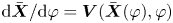 $\textrm {d}\bar {\boldsymbol {X}} / \textrm {d}\varphi = \boldsymbol {V}(\bar {\boldsymbol {X}}(\varphi ), \varphi )$ is always satisfied and
  $\Delta C = \Delta \mathcal {L}_C$ (from (3.7)), which gives
 \begin{equation} \Delta C ={-} \int_0^{2{\rm \pi} L / n_0} \textrm{d}\varphi \bar{\boldsymbol \lambda} \boldsymbol{\cdot} \Delta \boldsymbol{V}(\bar{\boldsymbol{X}}, \varphi) , \end{equation}
where
 \begin{equation} \Delta \boldsymbol{V} (\bar{\boldsymbol{X}}, \varphi) = \frac{\bar{R} \Delta \boldsymbol{B}_{p} (\bar{\boldsymbol{X}}, \varphi)}{B_{\varphi}(\bar{\boldsymbol{X}}, \varphi)} - \frac{\bar{R} \boldsymbol{B}_{p} (\bar{\boldsymbol{X}}, \varphi) \Delta B_{\varphi} (\bar{\boldsymbol{X}}, \varphi) }{B_{\varphi}(\bar{\boldsymbol{X}}, \varphi)^2 } . \end{equation}
3.2. Variation of  $\varSigma _k$

Upon varying the magnetic field from  $\boldsymbol {B}(\boldsymbol {R})$ to
  $\boldsymbol {B}(\boldsymbol {R}) + \Delta \boldsymbol {B}(\boldsymbol {R})$, the quantity
  $\varSigma _k$ in (2.62) varies owing to the variation of the eigenvectors
  $\hat {\boldsymbol {e}}_{\perp k}$ and
  $\hat {\boldsymbol {e}}_{\parallel k+q}$, and of the tangent map
  $\textsf {S}_k^q$,
 \begin{align} \Delta \varSigma_k = \sum_{q=q_0}^{q_0+L-1} \left( \hat{\boldsymbol{e}}_{{\parallel}, k+q } \boldsymbol{\cdot} \Delta \textsf {S}_k^q \boldsymbol{\cdot} \hat{\boldsymbol{e}}_{{\perp},k } + \Delta e_{{\parallel}, k+q} \hat{\boldsymbol{e}}_{{\perp} k+q} \boldsymbol{\cdot} \textsf {S}_k^q \boldsymbol{\cdot} \hat{\boldsymbol{e}}_{{\perp}, k } + \Delta e_{{\perp}, k} \hat{\boldsymbol{e}}_{{\parallel}, k+q} \boldsymbol{\cdot} \textsf {S}_k^q \boldsymbol{\cdot} \hat{\boldsymbol{e}}_{{\parallel} , k} \right) {.} \end{align}
In (3.15), we have used the fact that the variation of a unit vector is perpendicular to the unit vector itself to re-express the variation of the normalized eigenvectors of  $\textsf {W}_k$ as
  $\Delta \hat {\boldsymbol {e}}_{\perp , k} = \Delta e_{\perp , k} \hat {\boldsymbol {e}}_{\parallel , k}$ and
  $\Delta \hat {\boldsymbol {e}}_{\parallel , k} = \Delta e_{\parallel , k} \hat {\boldsymbol {e}}_{\perp , k}$. The slow rotation of nearby points around the O point gives
  $\sin ( 2{\rm \pi} \omega k / n_0 ) \simeq 1$ and
  $\cos ( 2{\rm \pi} \omega k / n_0 ) \simeq 0$. Thus, the matrix elements
  $\hat {\boldsymbol {e}}_{\perp , k+q} \boldsymbol {\cdot } \textsf {S}_k^q \boldsymbol {\cdot } \hat {\boldsymbol {e}}_{\perp , k}$ and
  $\hat {\boldsymbol {e}}_{\parallel , k+q} \boldsymbol {\cdot } \textsf {S}_k^q \boldsymbol {\cdot } \hat {\boldsymbol {e}}_{\parallel , k}$, equal to the diagonal matrix elements in
  $\textsf {S}_{R, k}^q$ ((2.31)), are both small in
  $2{\rm \pi} \omega L / n_0$. This gives
 \begin{equation} \Delta \varSigma_k \simeq \sum_{q=q_0}^{q_0+L-1} \hat{\boldsymbol{e}}_{{\parallel}, k+q } \boldsymbol{\cdot} \Delta \textsf {S}_k^q \boldsymbol{\cdot} \hat{\boldsymbol{e}}_{{\perp}, k } = \sum_{q=q_0}^{q_0+L-1} \hat{\boldsymbol{e}}_{{\parallel}, k+q } \boldsymbol{\cdot} \Delta \boldsymbol{s}_k^q {;} \end{equation}
here, we have introduced the variable  $\boldsymbol {s}_k(\varphi ) = \delta \boldsymbol {X} (\varphi ) / |\delta \boldsymbol {X}(2{\rm \pi} k / n_0)|$, which satisfies the differential equation (2.44),
 \begin{equation} \frac{\textrm{d}\boldsymbol{s}_k}{\textrm{d}\varphi} = \boldsymbol{s}_k \boldsymbol{\cdot} \boldsymbol{\nabla}_{\boldsymbol X} \boldsymbol{V} , \end{equation}
with boundary condition  $\boldsymbol {s}_k(2{\rm \pi} k / n_0) = \boldsymbol {s}_{ k}^0 = \hat {\boldsymbol {e}}_{\perp , k}$, and defined the variation
  $\Delta \boldsymbol {s}_k (\varphi )$. We re-express (3.16) as
 \begin{equation} \Delta \varSigma_k \simeq \sum_{Q=0}^{Q_0-1} \int_{2{\rm \pi} ( k + LQ) / n_0}^{2{\rm \pi} (k+L Q+ L) / n_0} \Delta \boldsymbol{s}_k (\varphi ) \boldsymbol{\cdot} \hat{\boldsymbol{e}}_{{\parallel}, k+q } \delta (\varphi - \varphi_{k+q} )\,\textrm{d}\varphi {,} \end{equation}
where the integer  $Q_0 = \lfloor q_0 / L \rfloor + 2$, with the brackets
  $\lfloor$ and
  $\rfloor$ denoting the floor function, is chosen such that all values of
  $q$ in the sum in (3.16) are counted. Introducing the notation
 \begin{equation} \left\langle \boldsymbol{A}_1 \boldsymbol{\cdot} \boldsymbol{A}_2 \right\rangle_{k,Q} = \int_{2{\rm \pi} (k+L Q) / n_0}^{2{\rm \pi} (k+L Q + L)/n_0} \boldsymbol{A}_1 \boldsymbol{\cdot} \boldsymbol{A}_2 \,\textrm{d}\varphi , \end{equation}
we define the Lagrangian of  $\varSigma _k$,
 \begin{align} \mathcal{L}_{\varSigma_k} = \varSigma_k + \sum_{Q=0}^{Q_0-1} \left( \left\langle \boldsymbol{\lambda}_{k,Q}, \frac{\textrm{d}\boldsymbol{X}}{\textrm{d}\varphi} - \boldsymbol{V}(\boldsymbol{X}, \varphi) \right\rangle_{k,Q} + \left\langle \boldsymbol{\mu}_k, \frac{\textrm{d}\boldsymbol{s}_k}{\textrm{d}\varphi} - \boldsymbol{s}_k \boldsymbol{\cdot} \boldsymbol{\nabla}_{\boldsymbol X} \boldsymbol{V} (\boldsymbol{X}, \varphi) \right\rangle_{k,Q} \right) . \end{align}
In (3.20), we have introduced two constraints using the adjoint variables  $\boldsymbol {\lambda }_{k,Q}(\varphi )$ and
  $\boldsymbol {\mu }_k (\varphi )$. With these constraints, the quantities
  $\mathcal {L}_{\varSigma _k}$ and
  $\varSigma _k$ are only equal to each other if
  $\boldsymbol {X} (\varphi )$ is a field line trajectory, which satisfies (2.41), and
  $\boldsymbol {s}_k$ satisfies the linearized equation (3.17) for small displacements about the field line.Footnote 2
Extremization with respect to variations in  $\boldsymbol {X} (\varphi )$ gives
 \begin{align} \Delta \mathcal{L}_{\varSigma_k} &={-} \sum_{Q=0}^{Q_0-1} \left\langle \Delta \boldsymbol{X}, \frac{\textrm{d}\boldsymbol{\lambda}_{k,Q}}{\textrm{d}\varphi} + \boldsymbol{\nabla}_{\boldsymbol X} \boldsymbol{V} \boldsymbol{\cdot} \boldsymbol{\lambda}_{k,Q} + \boldsymbol{s}_k \boldsymbol{\cdot} \boldsymbol{\nabla}_{\boldsymbol X} \boldsymbol{\nabla}_{\boldsymbol X} \boldsymbol{V} \boldsymbol{\cdot} \boldsymbol{\mu}_k \right\rangle \nonumber\\ &\quad + \sum_{Q=0}^{Q_0-1} \left[ \Delta \boldsymbol{X}(2{\rm \pi}(k+QL+L)/n_0) \boldsymbol{\cdot} \boldsymbol{\lambda}_{k,Q} (2{\rm \pi}(k+QL+L)/n_0) \right. \nonumber\\ &\quad - \left. \Delta \boldsymbol{X}(2{\rm \pi} (k + QL)/n_0) \boldsymbol{\cdot} \boldsymbol{\lambda}_{k,Q} (2{\rm \pi} (k+QL)/n_0) \right] = 0 , \end{align}
where the Hessian of the field-line-following equation (2.41) is
 \begin{align} \boldsymbol{\nabla}_{\boldsymbol X} \boldsymbol{\nabla}_{\boldsymbol X} \boldsymbol{V} (\boldsymbol{X}, \varphi) &= \frac{ 2 \hat{\boldsymbol{e}}_R \boldsymbol{\nabla}_{\boldsymbol X} \boldsymbol{B}_p (\boldsymbol{X}, \varphi) }{B_{\varphi} (\boldsymbol{X}, \varphi) } - \frac{ 2 \hat{\boldsymbol{e}}_R ( \boldsymbol{\nabla}_{\boldsymbol X} B_{\varphi} (\boldsymbol{X}, \varphi) ) \boldsymbol{B}_p (\boldsymbol{X}, \varphi) }{B_{\varphi}(\boldsymbol{X}, \varphi)^2} + \frac{ R\boldsymbol{\nabla}_{\boldsymbol X} \boldsymbol{\nabla}_{\boldsymbol X} \boldsymbol{B}_p (\boldsymbol{X}, \varphi) }{B_{\varphi}(\boldsymbol{X}, \varphi) } \nonumber\\ &\quad - \frac{ 2 R ( \boldsymbol{\nabla}_{\boldsymbol X} B_{\varphi}(\boldsymbol{X}, \varphi) ) ( \boldsymbol{\nabla}_{\boldsymbol X} \boldsymbol{B}_p (\boldsymbol{X}, \varphi) )}{B_{\varphi}(\boldsymbol{X}, \varphi)^2} - \frac{ R ( \boldsymbol{\nabla}_{\boldsymbol X} \boldsymbol{\nabla}_{\boldsymbol X} B_{\varphi}(\boldsymbol{X}_p, \varphi) ) \boldsymbol{B}_p(\boldsymbol{X}, \varphi) }{B_{\varphi}(\boldsymbol{X}, \varphi)^2} \nonumber\\ &\quad + \frac{ 2 R ( \boldsymbol{\nabla}_{\boldsymbol X} B_{\varphi} (\boldsymbol{X}, \varphi) ) ( \boldsymbol{\nabla}_{\boldsymbol X} B_{\varphi} (\boldsymbol{X}, \varphi) ) \boldsymbol{B}_p (\boldsymbol{X}, \varphi) }{B_{\varphi}(\boldsymbol{X}, \varphi)^3} {.} \end{align}
We consider  $\boldsymbol {X} (\varphi )$ to be a periodic field line
  $\bar {\boldsymbol {X}} (\varphi )$ (an island centre) after the variation of the magnetic field configuration, such that
  $\Delta \boldsymbol { X} ( 2{\rm \pi} (k+QL)/n_0 ) = \Delta \boldsymbol { X} ( 2{\rm \pi} (k+QL+L)/n_0 )$. Therefore, all the boundary terms in (3.21) vanish if
  $\boldsymbol {\lambda }_{k,Q} ( 2{\rm \pi} (k+QL)/n_0 ) = \boldsymbol {\lambda }_{k,Q} ( 2{\rm \pi} (k + QL + L)/n_0 )$. The adjoint equations for
  $\boldsymbol {\lambda }_{k,Q} (\varphi )$ are thus
 \begin{equation} \frac{\textrm{d}\boldsymbol{\lambda}_{k,Q}}{\textrm{d}\varphi} + \boldsymbol{\nabla}_{\boldsymbol X} \boldsymbol{V} \boldsymbol{\cdot} \boldsymbol{\lambda}_{k,Q} + \boldsymbol{s}_k \boldsymbol{\cdot} \boldsymbol{\nabla}_{\boldsymbol X} \boldsymbol{\nabla}_{\boldsymbol X} \boldsymbol{V} \boldsymbol{\cdot} \boldsymbol{\mu}_k = 0 , \end{equation}
to be solved for periodic solutions  $\bar { \boldsymbol \lambda }_{k,Q} ( \varphi )$ in the interval
  $2{\rm \pi} QL / n_0 \leqslant \varphi - 2{\rm \pi} k / n_0 \leqslant 2{\rm \pi} (QL+L) / n_0$ for all
  $k$ and
  $Q$.
$Q$.
Extremizing  $\mathcal {L}_{\varSigma _k}$, with respect to variations in
  $\boldsymbol {s}_k (\varphi )$, gives an equation for
  $\boldsymbol {\mu }_k$,
 \begin{align} \Delta \mathcal{L}_{\varSigma_k} &= \sum_{Q=0}^{Q_0-1} \left[ \left\langle \Delta \boldsymbol{s}_k , \sum_{q=q_0}^{q_0+L-1} \hat{\boldsymbol{e}}_{{\parallel} k+q} \delta ( \varphi - \varphi_{k+q} ) - \frac{d \boldsymbol{\mu}_k}{\textrm{d}\varphi} - \boldsymbol{\nabla}_{\boldsymbol X} \boldsymbol{V} \boldsymbol{\cdot} \boldsymbol{\mu}_k \right\rangle_Q \right] \nonumber\\ &\quad + \boldsymbol{\mu}_k (2{\rm \pi} (k+ L Q_0 )/n_0) \boldsymbol{\cdot} \Delta \boldsymbol{s}_{k} (2{\rm \pi} (k+L Q_0)/n_0)\notag\\ &\quad - \boldsymbol{\mu}_k (2{\rm \pi} k / n_0) \boldsymbol{\cdot} \Delta \boldsymbol{s}_{k} (2{\rm \pi} k / n_0) = 0 , \end{align}
where all boundary terms at  $\varphi = 2{\rm \pi} (k+LQ)/n_0$ for
  $Q\neq 0$ and
  $Q\neq Q_0$ have vanished because
  $\boldsymbol {\mu }_k$ is a continuous variable in the interval
  $2{\rm \pi} k / n_0 \leqslant \varphi \leqslant 2{\rm \pi} (k + Q_0L ) / n_0$. When considering variations in
  $\boldsymbol {s}_k$, the initial condition
  $\boldsymbol {s}_{k}(2{\rm \pi} k / n_0 ) = \boldsymbol {s}_k^0 = \hat {\boldsymbol {e}}_{\perp k}$ can be assumed to be unchanged and therefore
  $\Delta \boldsymbol {s}_k (2{\rm \pi} k / n_0) = 0$. Hence, the boundary terms in (3.24) vanish by imposing
  $\boldsymbol {\mu }_k ( 2{\rm \pi} (k+LQ_0)/n_0 ) = 0$, which results in the differential equation
 \begin{equation} \frac{\textrm{d} \boldsymbol{\mu}_k}{\textrm{d}\varphi} = \sum_{q=q_0}^{q_0+L-1} \hat{\boldsymbol{e}}_{{\parallel} k+q} \delta ( \varphi - \varphi_{k+q} ) - \boldsymbol{\nabla}_{\boldsymbol X} \boldsymbol{V} \boldsymbol{\cdot} \boldsymbol{\mu}_k . \end{equation}
Note that  $\boldsymbol {\mu }_k (2{\rm \pi} k / n_0)$ can be obtained from
  $\boldsymbol {\mu }_k (2{\rm \pi} (k+L Q_0) / n_0) = 0$ using (3.25). This can be solved by repeated applications of appropriate partial tangent maps and jump conditions at the angles
  $\varphi _{k+q}$; as shown in Appendix C, the linear mapping from
  $\boldsymbol \mu _k$ to
  $\boldsymbol \mu _{k+1}$ that follows from the homogeneous term on the right-hand side of (3.25) is the adjoint of the partial tangent map
  $\textsf {S}_k^1$, such that
  $\boldsymbol \mu _k ( 2{\rm \pi} (k+q)/L) = ( \textsf {S}_{k+q}^1 )^{\intercal } \boldsymbol {\cdot } \boldsymbol \mu _k ( 2{\rm \pi} (k+q+1)/L)$. The adjoint variables
  $\boldsymbol {\lambda }_{k,Q} (\varphi )$ can be obtained from (3.23) once the the adjoint variables
  $\boldsymbol {\mu }_k (\varphi )$ are obtained from (3.25).
The magnetic field configuration is varied while considering  $\bar { \boldsymbol X} (\varphi )$ to be the magnetic field line trajectory at the island centre, which satisfies (2.41) with a periodic boundary condition, and while constraining
  $\boldsymbol {s}_k (\varphi )$ to satisfy (3.17) for linearized trajectories about the island centre. We thus conclude that
  $\varSigma _k = \mathcal {L}_{\varSigma _k}$ and thus
  $\Delta \varSigma _k = \Delta \mathcal {L}_{\varSigma _k}$. Therefore, the variation of
  $\varSigma _k$ is given by
 \begin{equation} \Delta \varSigma_k ={-} \sum_{Q=0}^{Q_0-1} \int_{2{\rm \pi} k / n_0}^{2{\rm \pi} (k + QL)/n_0} \textrm{d}\varphi ( \bar{ \boldsymbol \lambda}_{k,Q} \boldsymbol{\cdot} \Delta \boldsymbol{V} (\bar{\boldsymbol{X}}, \varphi) + \boldsymbol{s}_{ k} \boldsymbol{\cdot} \boldsymbol{\nabla}_{\boldsymbol X} \Delta \boldsymbol{V} (\bar{\boldsymbol{X}}, \varphi) \boldsymbol{\cdot} \boldsymbol{\mu}_k ) , \end{equation}
where  $\bar {\boldsymbol \lambda }_{k,Q}$ is a periodic solution of (3.23) and
  $\boldsymbol {\mu }_k$ is the solution of (3.25), which satisfies the boundary condition
  $\boldsymbol {\mu }_k (2{\rm \pi} (k+L Q_0) / n_0) = 0$. The function
  $\boldsymbol {\nabla }_{\boldsymbol X} \Delta \boldsymbol {V} (\bar {\boldsymbol {X}}, \varphi )$ can be written explicitly in terms of variations of the magnetic field and its gradients by differentiating (3.14),
 \begin{align} \boldsymbol{\nabla}_{\boldsymbol X} \Delta \boldsymbol{V} (\bar{\boldsymbol{X}}, \varphi) &= \frac{\hat{\boldsymbol{e}}_R \Delta \boldsymbol{B}_p (\bar{\boldsymbol{X}}, \varphi) }{B_{\varphi} (\bar{\boldsymbol{X}}, \varphi) } - \frac{\hat{\boldsymbol{e}}_R \boldsymbol{B}_p(\bar{\boldsymbol{X}}, \varphi) \Delta B_{\varphi} (\bar{\boldsymbol{X}}, \varphi) }{B_{\varphi} (\bar{\boldsymbol{X}}, \varphi)^2 }+ \frac{R \boldsymbol{\nabla}_{\boldsymbol X} \Delta \boldsymbol{B}_p (\bar{\boldsymbol{X}}, \varphi) }{B_{\varphi} (\bar{\boldsymbol{X}}, \varphi) } \nonumber\\ &\quad - \frac{R (\boldsymbol{\nabla}_{\boldsymbol X} \boldsymbol{B}_p (\bar{\boldsymbol{X}}, \varphi) ) \Delta B_{\varphi} (\bar{\boldsymbol{X}}, \varphi) }{B_{\varphi}(\bar{\boldsymbol{X}}, \varphi)^2} - \frac{R \boldsymbol{\nabla}_{\boldsymbol X} B_{\varphi} (\bar{\boldsymbol{X}}, \varphi) \Delta \boldsymbol{B}_p (\bar{\boldsymbol{X}}, \varphi) }{B_{\varphi}(\bar{\boldsymbol{X}}, \varphi)^2} \nonumber\\ &\quad - \frac{R \boldsymbol{\nabla}_{\boldsymbol X} (\Delta B_{\varphi } (\bar{\boldsymbol{X}}, \varphi) ) \boldsymbol{B}_p (\bar{\boldsymbol{X}}, \varphi) }{B_{\varphi}(\bar{\boldsymbol{X}}, \varphi)^2} + \frac{2 R (\boldsymbol{\nabla}_{\boldsymbol X} B_{\varphi } ) \boldsymbol{B}_p \Delta B_{\varphi} }{B_{\varphi}^3} . \end{align}
3.3. Residue variation
The residue  $\mathcal {R}$ varies owing to the variation of the full-orbit tangent map
  $\textsf {M}_k$. We re-express the trace of the full-orbit tangent map as
 \begin{equation} \textrm{Tr} (\textsf {M}_0) = \textsf {I} : \textsf {M}_0 , \end{equation}
where the operation denoted by the colon  $:$ corresponds to multiplying each matrix element of one matrix with the corresponding matrix element of the other matrix and adding the results together. Note that
  $k=0$ was chosen in (3.28), as the residue is independent of
  $k$. From (2.54) and (3.28), we obtain
 \begin{equation} \Delta \mathcal{R} ={-} \tfrac{1}{4} \textsf {I} : \Delta \textsf {M}_0 {.} \end{equation}
Recall that  $\textsf {M}_0 = \textsf {S}_0 ( 2{\rm \pi} L / n_0 )$ and that the tangent map
  $\textsf {S}_0$ satisfies the differential equation (2.46) with boundary condition
  $\textsf {S}_0(0) = \textsf {I}$. We define the Lagrangian of
  $\mathcal {R}$,
 \begin{align} \mathcal{L}_{\mathcal{R}} = \mathcal{R} + \int_0^{2{\rm \pi} L / n_0} \textrm{d}\varphi \left[ \boldsymbol{\lambda}_{\mathcal{R}} \boldsymbol{\cdot} \left( \frac{\textrm{d}\boldsymbol{X}}{\textrm{d}\varphi} - \boldsymbol{V}(\boldsymbol{X}, \varphi) \right) + \boldsymbol{\mu}_{\mathcal{R}} : \left( \frac{\textrm{d}\textsf {S}_0}{\textrm{d}\varphi} - \left( \boldsymbol{\nabla}_{\boldsymbol X} \boldsymbol{V} (\boldsymbol{X}, \varphi) \right)^\intercal \boldsymbol{\cdot} \textsf {S}_0 \right) \right] . \end{align}
In (3.30), we have introduced two constraints using the adjoint variables  $\boldsymbol {\lambda }_{\mathcal {R}}(\varphi )$ (a vector) and
  $\boldsymbol{\mu} _{\mathcal {R}} (\varphi )$ (a matrix). With these constraints, the quantities
  $\mathcal {L}_{\mathcal {R}}$ and
  $\mathcal {R}$ are equal to each other if
  $\boldsymbol {X} (\varphi )$ is a field line trajectory, which satisfies (2.41), and
  $\textsf {S}_0$ satisfies (2.46) for the tangent map.
Extremization with respect to variations in  $\boldsymbol {X} (\varphi )$ gives
 \begin{align} \Delta \mathcal{L}_{\mathcal{R}} &={-} \left\langle \Delta \boldsymbol{X}, \frac{\textrm{d}\boldsymbol{\lambda}_{\mathcal{R}}}{\textrm{d}\varphi} + \boldsymbol{\nabla}_{\boldsymbol X} \boldsymbol{V} \boldsymbol{\cdot} \boldsymbol{\lambda}_{\mathcal{R}} + \left( \boldsymbol{\nabla}_{\boldsymbol X} \boldsymbol{\nabla}_{\boldsymbol X} \boldsymbol{V} \boldsymbol{\cdot} \boldsymbol{\mu}_{\mathcal{R}} \right) : \textsf {S}_0 \right\rangle \nonumber\\ &\quad + \Delta \boldsymbol{X}(2{\rm \pi} L/n_0) \boldsymbol{\cdot} \boldsymbol{\lambda}_{\mathcal{R}} (2{\rm \pi} L/n_0) - \Delta \boldsymbol{X}(0) \boldsymbol{\cdot} \boldsymbol{\lambda}_{\mathcal{R}} (0) = 0 , \end{align}
Again, all the boundary terms in (3.31) vanish if  $\boldsymbol {\lambda }_{\mathcal {R}} ( 2{\rm \pi} L/n_0 ) = \boldsymbol {\lambda }_{\mathcal {R}} ( 0 )$. The adjoint equation for
  $\boldsymbol {\lambda }_{\mathcal {R}} (\varphi )$ is thus
 \begin{equation} \frac{\textrm{d}\boldsymbol{\lambda}_{\mathcal{R}}}{\textrm{d}\varphi} + \boldsymbol{\nabla}_{\boldsymbol X} \boldsymbol{V} \boldsymbol{\cdot} \boldsymbol{\lambda}_{\mathcal{R}} + \left( \boldsymbol{\nabla}_{\boldsymbol X} \boldsymbol{\nabla}_{\boldsymbol X} \boldsymbol{V} \boldsymbol{\cdot} \boldsymbol{\mu}_{\mathcal{R}} \right) : \textsf {S}_0 = 0 , \end{equation}
to be solved in the interval  $0 \leqslant \varphi \leqslant 2{\rm \pi} L / n_0$ for periodic solutions, denoted
  $\bar { \boldsymbol \lambda }_{\mathcal {R}} (\varphi )$.
Extremizing  $\mathcal {L}_{\mathcal {R}}$ with respect to variations in
  $\textsf {S}_0 (\varphi )$ gives an equation for
  $\boldsymbol \mu _{\mathcal {R}}$,
 \begin{equation} \Delta \mathcal{L}_{\mathcal{R}} ={-} \frac{1}{4} \textsf {I} : \Delta \textsf {M}_0 + \left\langle \boldsymbol{\mu}_{\mathcal{R}} , \frac{\textrm{d} \Delta \textsf {S}_0 }{\textrm{d}\varphi} - (\boldsymbol{\nabla}_{\boldsymbol X} \boldsymbol{V})^\intercal \boldsymbol{\cdot} \Delta \textsf {S}_0 \right\rangle = 0 . \end{equation}
Note that we have used the following definition for the inner product of two matrix quantities,
 \begin{equation} \left\langle \textsf {A}_1, \textsf {A}_2 \right\rangle = \int_0^{2{\rm \pi} L / n_0}\, \textrm{d}\varphi \textsf {A}_1 : \textsf {A}_2 . \end{equation}
We re-express (3.33) as
 \begin{gather} -\frac{1}{4} \textsf {I} : \Delta \textsf {M}_0 - \left\langle \Delta \textsf {S}_0 , \frac{\textrm{d} \boldsymbol{\mu}_{\mathcal{R}} }{\textrm{d}\varphi} + \boldsymbol{\nabla}_{\boldsymbol X} \boldsymbol{V} \boldsymbol{\cdot} \boldsymbol \mu_{\mathcal{R}} \right\rangle + \boldsymbol \mu_{\mathcal{R}} (2{\rm \pi} L / n_0 ) : \Delta S_0 ( 2{\rm \pi} L / n_0 ) \nonumber\\ \quad - \boldsymbol \mu_{\mathcal{R}} (0 ) : \Delta S_0 ( 0 ) = 0 . \end{gather}
Noting that  $\Delta \textsf {S}_0 (0) = 0$ and
  $\Delta S_0 (2{\rm \pi} L / n_0 ) = \Delta \textsf {M}_0$ both hold true by definition, the boundary terms are zero provided
  $\boldsymbol \mu _{\mathcal {R}} ( 2{\rm \pi} L / n_0 ) = \textsf {I}/4$ is chosen. Thus, the adjoint equation for
  $\mu _{\mathcal {R}}$ is
 \begin{equation} \frac{\textrm{d} \boldsymbol{\mu}_{\mathcal{R}} }{\textrm{d}\varphi} ={-} \boldsymbol{\nabla}_{\boldsymbol X} \boldsymbol{V} \boldsymbol{\cdot} \boldsymbol \mu_{\mathcal{R}}, \end{equation}
with  $\boldsymbol \mu _{\mathcal {R}} ( 2{\rm \pi} L / n_0 ) = \textsf {I}/4$ as a boundary condition. From Appendix C, an equivalent form of this boundary condition is
  $\boldsymbol \mu _{\mathcal {R}} ( 0 ) = (\textsf {M}_0^{\intercal })/4$.
As before, the variation of the residue is given by
 \begin{equation} \Delta \mathcal{R} ={-} \int_0^{2{\rm \pi} L /n_0} \left( \bar{\boldsymbol \lambda}_{\mathcal{R}} \boldsymbol{\cdot} \Delta \boldsymbol{V} (\bar{\boldsymbol{X}}, \varphi) + ( \boldsymbol{\nabla}_{\boldsymbol X} \Delta \boldsymbol{V} (\bar{\boldsymbol{X}}, \varphi) \boldsymbol{\cdot} \boldsymbol{\mu}_{\mathcal{R}} ) : \textsf {S}_0 \right) \,\textrm{d}\varphi , \end{equation}
where  $\bar { \boldsymbol \lambda }_{\mathcal {R}}$ and
  $\boldsymbol{\mu} _{\mathcal {R}}$ are the solutions of the adjoint equations (3.23) and (3.25) with the appropriate boundary conditions.
To conclude this section, we briefly discuss a subsidiary result of the preceding analysis. The trace of the full-orbit tangent map calculated at the magnetic axis is related the rotation angle of nearby trajectories about the magnetic axis. By definition, this is proportional to the on-axis rotational transform. Equating (2.52) (with  $k=0$) to the product of the interval in toroidal angle,
  $2{\rm \pi} / n_0$, and the on-axis rotational transform,
  $\bar {\iota }$, and re-arranging for
  $\bar {\iota }$, gives
 \begin{equation} \bar{\iota} = \frac{n_0}{2{\rm \pi}} \arccos \left( \frac{1}{2} \textrm{Tr} \left( \textsf {M}_0 \right) \right) \rm . \end{equation}
Note that this equation is correct provided  $\bar {\iota } < {n_0}/{2}$, a condition which is satisfied in most stellarators. Remembering the definition (2.54) of the residue, the variation of the on-axis rotational transform is given by
 \begin{equation} \Delta \bar{\iota} = \frac{n_0}{{\rm \pi} \sin \left( 2{\rm \pi} \bar{\iota} / n_0 \right)} \Delta \mathcal{R} . \end{equation}
4. Numerical results
In this section, we present the numerical results obtained for the gradients of the island width and of other properties of the periodic field line. In § 4.1, we briefly explain the numerical scheme used to obtain our results. We then present, in § 4.2, numerical results for the island width, its gradient and the gradient of other island-related quantities in an analytical magnetic configuration studied by Reiman & Greenside (Reference Reiman and Greenside1986). In § 4.3, we present results for the shape gradient of the width of a magnetic island in NCSX with respect to the positions on a type-A modular coil. Finally, in § 4.4, we apply the gradient of the residue of a periodic field line to optimize a helical magnetic configuration of the kind studied by Cary & Hanson (Reference Cary and Hanson1986) and Hanson & Cary (Reference Hanson and Cary1984).
4.1. Numerical scheme
A Runge–Kutta fourth-order explicit scheme is used to integrate equations (2.41), (2.46), (3.12), (3.23) and (3.25) in toroidal angle  $\varphi$. The number of grid points in
  $\varphi$ per field period is denoted
  $N_{\varphi }$, such that the number of grid points per toroidal turn is
  $n_0 N_{\varphi }$.
A Newton method is used to search for periodic solutions of the magnetic field line such as the magnetic axis and a magnetic island centre. The search proceeds as follows. The position of the periodic field line is initially guessed as  $\boldsymbol {X}^0 (0)$ and equation (2.41) is integrated in
  $\varphi$ from
  $\varphi = 0$ to
  $\varphi = 2{\rm \pi} L / n_0$, where
  $L$ is an integer (
 $=1$ for the magnetic axis). The tangent map is also integrated following the magnetic field line. The final position
  $\boldsymbol {X}( 2{\rm \pi} L / n_0 )$ and tangent map
  $\textsf {S} ( 2{\rm \pi} L / n_0 )$ are used to evaluate a next guess for the magnetic axis as follows. The step
  $\boldsymbol {X}_\textrm {step} (0)$ in position necessary to move closer to the periodic solution at the next iteration,
  $\boldsymbol {X}^{i+1} (0) = \boldsymbol {X}^{i} (0) + \boldsymbol {X}^i_\textrm {step} (0)$, is calculated by imposing
  $\boldsymbol {X}^i(0) + \boldsymbol {X}^i_\textrm {step} (0) = \boldsymbol {X}^i ( 2{\rm \pi} L / n_0 ) + \boldsymbol {X}^i_\textrm {step} ( 2{\rm \pi} L / n_0 )$ on the linearized equations. This leads to
  $\boldsymbol {X}^i(0) + \boldsymbol {X}_\textrm {step}^i(0) = \boldsymbol {X}^i( 2{\rm \pi} L / n_0 ) + \textsf {S}^i ( 2{\rm \pi} L / n_0 ) \boldsymbol {\cdot } \boldsymbol {X}^i_\textrm {step}(0)$ and, upon rearranging, to
 \begin{equation} \boldsymbol{X}_\textrm{step}^i (0) = ( \textsf {I} - \textsf {S}^i ( 2{\rm \pi} L / n_0 ) )^{{-}1} \boldsymbol{\cdot} ( \boldsymbol{X}^i ( 2{\rm \pi} L / n_0 ) - \boldsymbol{X}^i(0) ) . \end{equation}
The error is calculated from
 \begin{equation} \mathcal{E}_i = \frac{\left| \boldsymbol{X}^i ( 2{\rm \pi} L / n_0 ) - \boldsymbol{X}^i (0) \right|}{\left| \boldsymbol{X}^i (0) \right|} \end{equation}
where the magnitude of the poloidal vector  $\boldsymbol {X} = (R, Z)$ is defined as
  $|\boldsymbol {X} | = \sqrt {R^2 + Z^2}$. A periodic field line solution is found if
  $\mathcal {E}_i$ falls below a threshold value
  $\mathcal {E}_\textrm {thresh} = 10^{-13}$; we then consider
  $\bar {\boldsymbol {X}}(\varphi ) = \boldsymbol {X}^i (\varphi )$.
Once a periodic field line is found, the values of the magnetic field and its first and second derivatives on the toroidal grid points and in the intermediate Runge–Kutta steps are stored to accelerate subsequent parts of the code such as the solutions of the adjoint equations and the calculations of the gradients.
4.2. Island width and gradient calculation: Reiman model
We study the magnetic configurations of a form similar to the model field used in § 5 of Reiman & Greenside (Reference Reiman and Greenside1986), given by (2.1) with
 \begin{gather} \psi = \tfrac{1}{2} r^2 , \end{gather}
 \begin{gather} \chi = \iota_\textrm{ax} \psi + \iota'_\textrm{ax} \psi^2 - \sum_{k=1}^{k_\textrm{max}} \varepsilon_k (2\psi)^{k/2} \cos \left( k \theta - \varphi \right) , \end{gather}
where  $k_\textrm {max}$ is the largest value of
  $k$ for which
  $\varepsilon _k \neq 0$. Here,
  $r$ and
  $\theta$ are chosen to be the poloidal minor radius and the geometric poloidal angle, such that
 \begin{equation} r = \sqrt{ \left( R - 1 \right)^2 + Z^2 }, \end{equation}
and
 \begin{equation} \tan \theta = \frac{Z}{ R - 1 } . \end{equation}
The explicit expressions for the magnetic field and its derivatives are derived from (2.1) and (4.3)–(4.6), and are given in Appendix D. The unperturbed configuration ( $\varepsilon _k = 0$ for all
  $k$) is symmetric in the geometric poloidal and toroidal angles (it is not curl-free and is therefore not a vacuum magnetic configuration). For the scope of this paper, we focus on the set of parameters
  $\iota _\textrm {ax} = 0.15$,
  $\iota '_\textrm {ax} = 0.38$ and
  $\varepsilon _k = 0$ for
  $k\neq 6$. In figure 1, we show a Poincaré plot of the island chain in the plane
  $\varphi = 0$, which results from the parameters
  $\varepsilon _6 = 0.01$ and
  $\varepsilon _6 = 0.001$.
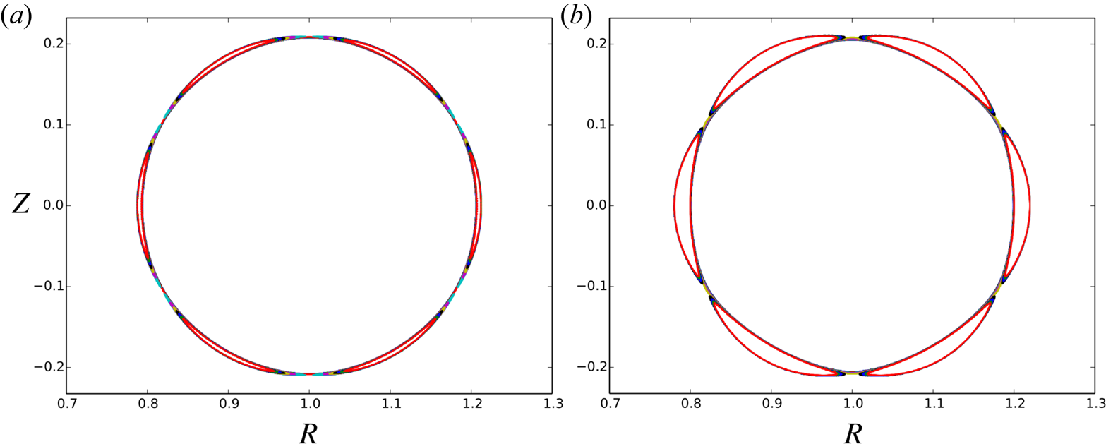
Figure 1. Poincaré plots showing magnetic field lines near the island separatrix in the Reiman magnetic field configuration with  $\iota _\textrm {ax} = 0.15$,
  $\iota '_\textrm {ax} = 0.38$ and
  $\varepsilon _i = 0$ for
  $i\neq 6$, for
  $\varepsilon _6 = 0.001$ (a) and
  $\varepsilon _6 = 0.01$ (b).
Although the Reiman magnetic field configuration is an experimentally unrealistic one, it is extremely useful and convenient to test the island width calculation presented in § 2. Taking  $\varepsilon _k = 0$ for
  $k \neq 6$ in (4.4) results in (2.2) with
 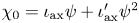 $\chi _0 = \iota _\textrm {ax} \psi + \iota '_\textrm {ax} \psi ^2$ and
  $\chi _1 = \varepsilon _6 (2\psi )^{3} \cos ( k \theta - \varphi + {\rm \pi})$. The (unperturbed) minor radius of the island chain is obtained by calculating
  $r = \bar {r}$ at the resonance,
  $\iota _\textrm {res}= 1/6 = \iota _\textrm {ax} + \iota '_\textrm {ax} \bar {r}^2$, which gives
  $\bar {r} = \sqrt {(\iota _\textrm {res} - \iota _\textrm {ax} )/\iota '_\textrm {ax}}$ and
  $\psi _0 = (\iota _\textrm {res} - \iota _\textrm {ax} )/(2\iota '_\textrm {ax})$. Therefore, the circumference of the unperturbed resonant flux surface section in the Reiman model is
 \begin{equation} \bar{C} = 2{\rm \pi} \sqrt{\frac{ \iota_\textrm{res} - \iota_\textrm{ax} }{\iota'_\textrm{ax}} } . \end{equation}
The width of the island chain expressed in the magnetic coordinate  $\psi$, obtained by inserting
  $\epsilon (\psi _0) = \varepsilon _6 ( (\iota _\textrm {res} - \iota _\textrm {ax} )/\iota '_\textrm {ax} )^3$ and
  $\iota _0'(\psi _0) = 2\iota '_\textrm {ax}$ into (2.23), is
 \begin{equation} \varUpsilon = 4 \sqrt{ \frac{ \varepsilon_6 }{ 2\iota'_\textrm{ax} } } \left( \frac{\iota_\textrm{res} - \iota_\textrm{ax} }{\iota'_\textrm{ax}} \right)^{3/2} . \end{equation}
From (2.32) and the equality  $\partial \xi _{\perp } / \partial \psi = \textrm {d} r / \textrm {d}\psi = 1/\bar {r}$, the expression for the island width in terms of the parameters of the Reiman model is
 \begin{equation} \bar{w}_{{\perp}} = 4 \sqrt{ \frac{ \varepsilon_6 }{ 2\iota'_\textrm{ax} } } \frac{\iota_\textrm{res} - \iota_\textrm{ax} }{\iota'_\textrm{ax}} . \end{equation}
Note that the subscript  $k$ in
  $w_{\perp , k}$ is unnecessary here, because the poloidal symmetry of the Reiman model implies that the width of all islands in the chain is identical.
In figure 2, we plot the island width calculated using (2.68) and compare it with that calculated using (4.9). The discrepancy between the two equations is almost entirely a result of the chord approximation for the circumference in (2.65).Footnote 3 This can be seen by comparing the island width calculated using the two methods with the quantity  $\bar {C} w_{\perp } / C$, a corrected island width where the sum of chords in (2.65) is replaced with the more accurate measure of the circumference in (4.7). The corrected island width has a near-perfect overlap with the width calculated from (4.9). The error between the two quantities decreases with
  $\varepsilon _6$ – consistent with the discussion in the final paragraph of § 2 (recall that (4.9) comes from (2.32)) – and is thus limited by the accuracy of the small island analysis. Conversely, the uncorrected island width
  $w_{\perp }$ is a less accurate approximation, as seen by the saturation of the error with decreasing
  $\varepsilon _6$. This arises from the chord approximation of the circumference limiting the accuracy of the island width evaluation, as the
  $O(L^{-1})$ error is dominant at sufficiently small
  $\varepsilon _6 \propto \hat {\epsilon }$.
Figure 2. Width of magnetic islands at the resonant flux surface with rotational transform  $\iota _\textrm {res} = 1/6$ calculated for the Reiman model magnetic field with
  $\iota _\textrm {ax} = 0.15$,
  $\iota '_\textrm {ax} = 0.38$ and
  $\varepsilon _i = 0$ for
  $i\neq 6$, shown as a function of
  $\varepsilon _6$. (a) Uncorrected
  $w_{\perp }$ (
 $\times$) and corrected
  $w_{\perp } \bar {C} / C$ (+) computed values of width are compared with the analytical value
  $\bar {w}_{\perp }$ in (4.9) (solid line). Here,
  $w_{\perp }$ is calculated from (2.68),
  $C$ from (2.65) and
  $\bar {C}$ from (4.7). (b) Normalized error
  $| 1 - w_{\perp } / \bar {w}_{\perp }|$ (
 $\times$) and
  $| 1 - w_{\perp } \bar {C} / (\bar {w}_{\perp } C)|$ (+). For
  $\varepsilon _6 > 10^{-7}$, the error in the corrected width decreases linearly with
  $\varepsilon _6$, as expected from the discussion at the end of § 2. For smaller values of
  $\varepsilon _6$, this error changes sign and increases with
  $\varepsilon _6^{-2}$, most likely owing to round-off error propagation. One in five markers are shown in both plots. The toroidal angle resolution is
  $N_{\varphi } = 80$.
The gradient of the island width with respect to the parameters  $\kappa \in \lbrace \iota _\textrm {ax}, \iota '_\textrm {ax}, \varepsilon _6\rbrace$ is calculated using the method derived in this paper. When one such parameter is varied infinitesimally, the infinitesimal magnetic field variation can be expressed as
  $\Delta \boldsymbol {B} = \Delta \kappa \partial \boldsymbol {B} / \partial \kappa$, where
  $\partial \boldsymbol {B} / \partial \kappa$ is the gradient of the magnetic field with respect to
  $\kappa$. The infinitesimal variation of the magnetic field gradient can be expressed as
  $\Delta \boldsymbol {\nabla }_{\boldsymbol X} \boldsymbol {B} = \Delta \kappa \partial (\boldsymbol {\nabla }_{\boldsymbol X} \boldsymbol {B}) / \partial \kappa$. Both
  $\partial \boldsymbol {B} / \partial \kappa$ and
  $\partial (\boldsymbol {\nabla }_{\boldsymbol X} \boldsymbol {B}) / \partial \kappa$ are straightforwardly obtained from the equations in Appendix D. The variation of the circumference and of the tangent map can also be expressed as
  $\Delta C = \Delta \kappa \partial C / \partial \kappa$ and
  $\Delta \varSigma _k = \Delta \kappa \partial \varSigma _k / \partial \kappa$. Thus, the gradient of the circumference, with respect to
  $\kappa$, is
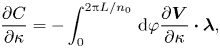 \begin{equation} \frac{\partial C }{\partial \kappa } ={-} \int_0^{2{\rm \pi} L / n_0}\,\textrm{d}\varphi \frac{\partial \boldsymbol{V}}{\partial \kappa} \boldsymbol{\cdot} \boldsymbol{\lambda} , \end{equation}
and the gradient of  $\varSigma _k$ is
 \begin{equation} \frac{\partial \varSigma_k}{\partial \kappa} ={-} \sum_{Q=0}^{Q_0-1} \int_{2{\rm \pi} (k + LQ)/n_0}^{2{\rm \pi} (k+ LQ+L)/n_0} \left( \frac{\partial \boldsymbol{V}}{\partial \kappa} \boldsymbol{\cdot} \boldsymbol{\lambda}_Q + \boldsymbol{s}_{{\perp} k} \boldsymbol{\cdot} \left( \frac{\partial \boldsymbol{\nabla}_{\boldsymbol X} \boldsymbol{V}}{\partial \kappa}\right) \boldsymbol{\cdot} \boldsymbol{\mu} \right) , \end{equation}
where
 \begin{gather} \frac{\partial \boldsymbol{V}}{\partial \kappa} = \frac{R }{B_{\varphi}} \frac{\partial \boldsymbol{B}_{p}}{\partial \kappa} - \frac{R \boldsymbol{B}_{p} }{B_{\varphi}^2 } \frac{ \partial B_{\varphi} }{\partial \kappa } , \end{gather}
 \begin{gather} \boldsymbol{\nabla}_{\boldsymbol X} \frac{\partial \boldsymbol{V}}{\partial \kappa } = \frac{\hat{\boldsymbol{e}}_R }{B_{\varphi}} \frac{\partial \boldsymbol{B}}{\partial \kappa } - \frac{\hat{\boldsymbol{e}}_R \boldsymbol{B}_{p}}{B_{\varphi}^2} \frac{\partial B_{\varphi}}{\partial \kappa } + \frac{R \boldsymbol{\nabla}_{\boldsymbol X} }{B_{\varphi}} \frac{\partial \boldsymbol{B}_{p}}{\partial \kappa } - \frac{R (\boldsymbol{\nabla}_{\boldsymbol X} \boldsymbol{B}_{p} ) }{B_{\varphi}^2} \frac{\partial B_{\varphi}}{\partial \kappa } - \frac{R (\boldsymbol{\nabla}_{\boldsymbol X} B_{\varphi}) }{B_{\varphi}^2} \frac{\partial \boldsymbol{B}}{\partial \kappa } \nonumber\\ - \left( \boldsymbol{\nabla}_{\boldsymbol X} \frac{\partial B_{\varphi}}{\partial \kappa } \right) \frac{R \boldsymbol{B}_{p} }{B_{\varphi}^2} + \frac{2 R (\boldsymbol{\nabla}_{\boldsymbol X} B_{\varphi } ) \boldsymbol{B}_{p} }{B_{\varphi}^3} \frac{\partial B_{\varphi} }{\partial \kappa } . \end{gather}
Hence, and by using (3.1), the gradient of the island width is given by
 \begin{equation} \frac{\partial \ln w_k }{\partial \kappa } = \frac{ \partial \ln C }{\partial \kappa} - \frac{\partial \ln \varSigma_k }{\partial \kappa } {,} \end{equation}
with  $\partial C / \partial \kappa$ and
  $\partial \varSigma _k / \partial \kappa$ given by (4.10) and (4.11), respectively. The gradient of the residue of a periodic field line follows from (3.37),
 \begin{equation} \frac{\partial \mathcal{R}}{\partial \kappa} ={-} \int_0^{2{\rm \pi} L /n_0} \left( \boldsymbol{\lambda}_{\mathcal{R}} \boldsymbol{\cdot} \frac{\partial \boldsymbol{V}}{\partial \kappa} + \left( \frac{\partial \boldsymbol{\nabla}_{\boldsymbol X} \boldsymbol{V} }{\partial \kappa } \boldsymbol{\cdot} \mu \right) : \textsf {S}_0 \right)\, \textrm{d}\varphi . \end{equation}
Considering the residue at the magnetic axis, the gradient of the on-axis rotational transform follows from (3.39),
 \begin{equation} \frac{\partial \bar{\iota}}{\partial \kappa} = \frac{n_0}{{\rm \pi} \sin \left( 2{\rm \pi} \bar{\iota} / n_0 \right)} \frac{\partial \mathcal{R}}{\partial \kappa} . \end{equation}
where  $\bar {\iota }$ is obtained from (3.38) and is found to be equal to
  $\iota _\textrm {ax}$, as expected.
The results of (4.10), (4.11), (4.14) and (4.15) can be compared with a numerical derivative of the quantities  $C$,
$C$,  $\varSigma _k$,
  $w_{\perp , k}$ and
  $\mathcal {R}$ calculated using finite differences. To this end, we calculate centred difference (CD) derivatives of the form
 \begin{equation} \frac{\partial^\textrm{CD} \ln f}{\partial \kappa} (\kappa, \delta ) = \frac{ \ln \left[f \left( \kappa + \delta \right) \right] - \ln \left[f \left( \kappa - \delta \right) \right] }{ 2\delta } . \end{equation}
The error with respect to the adjoint calculation of the derivative in (4.17) is
 \begin{equation} E_{f} (\delta ) = \left| \frac{\partial^\textrm{CD} \ln f}{\partial \kappa} (\kappa, \delta ) - \frac{ \partial \ln f }{ \partial \kappa } (\kappa ) \right| \end{equation}
In (4.17)–(4.18),  $f \in \lbrace \mathcal {R}, C, \varSigma _k, w_{\perp , k} \rbrace$. We expect the centred difference derivative of the numerically calculated island width to approach the numerically calculated derivative as
  $\delta$ is decreased. Having ignored the parts of the derivative of
  $\varSigma _k$ that are small in
  $\hat {\epsilon }$ in (3.15), one might expect that
  $E(\delta ) \sim \delta ^2$ for
  $\delta$ larger than a threshold value and
  $E(\delta ) \sim \hat {\epsilon }$ for smaller
  $\delta$. However, comparing the Reiman model to the derivation of the island width, the quantity
  $\zeta _0 ( \psi )$ is independent of
  $\psi$ in the Reiman model. Thus, the diagonal elements of the tangent map in (2.17), and correspondingly the off-diagonal elements of the scalar invariant matrix in (2.26), are exactly zero. Hence, the eigenvectors
  $\hat {\boldsymbol {e}}_{\perp }$ and
  $\hat {\boldsymbol {e}}_{\parallel }$ are exactly aligned with
  $\boldsymbol {\nabla }_{\boldsymbol X} \psi$ and
  $\boldsymbol {\nabla }_{\boldsymbol X} \theta$, respectively, for any value of the parameters
  $\iota _\textrm {ax}$,
  $\iota '_\textrm {ax}$ and
  $\varepsilon _6$. Thus, the small terms in
  $\hat {\epsilon }$ that were neglected in the derivation of the gradient of the island width are exactly zero in the Reiman model, and
  $E(\delta ) \sim \delta ^2$ should hold for all values of
  $\delta$. In figure 3, the quantity
  $E_{f} (\delta )$ for
  $f\in \lbrace \mathcal {R}, C, \varSigma , w_{\perp } \rbrace$ is shown for derivatives with respect to
 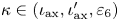 $\kappa \in (\iota _\textrm {ax}, \iota '_\textrm {ax}, \varepsilon _6 )$ for
  $\iota _\textrm {ax} = 0.15$,
  $\iota '_\textrm {ax} = 0.38$ and
  $\varepsilon _6 = 0.01$. The proportionality
  $E_{f} (\delta ) \propto \delta ^2$ for all
  $\kappa$ is strong evidence that the gradient calculation is accurate for all quantities. In addition, the gradient of the on-axis rotational transform
  $\bar {\iota }$ calculated from (4.16) is, as expected, unity for
  $\kappa = \iota _\textrm {ax}$ and zero for
  $\kappa \in \lbrace \iota _\textrm {ax}', \varepsilon _6 \rbrace$.
Figure 3. Errors, relative to a centred difference approximation, in the gradients of residue  $\mathcal {R}$, circumference
  $C$,
$C$,  $\varSigma$ and island width
  $w_{\perp }$ calculated with respect to the on-axis rotational transform
  $\iota _\textrm {ax}$, its first derivative
  $\iota _\textrm {ax}'$ and the amplitude of the resonant perturbation
  $\varepsilon _6$ in the Reiman model. The errors
  $E(\delta )$, defined in (4.18), are shown as a function of a normalized finite-difference step size
  $\mathcal {R}^{-1} ( \partial \mathcal {R} / \partial \kappa ) \delta$. The configuration parameters are
  $\iota _\textrm {ax} = 0.15$,
  $\iota '_\textrm {ax} = 0.38$,
  $\varepsilon _6 = 0.01$ and
  $\varepsilon _i = 0$ for
  $i\neq 6$. The resonant flux surface has the rotational transform
  $\iota _\textrm {res} = 1/6$. The dashed line is
  $E(\delta ) = \delta ^2$. The toroidal angle resolution is
  $N_{\varphi } = 80$.
4.3. Shape gradient calculation: explicit coils
In this section, it will be useful to denote the position along a magnetic field line, expressed in a set of right-handed Cartesian coordinates, as  $\boldsymbol{R} = (X, Y, Z)$. The coordinate
  $Z$ is the same as in the two-dimensional vector
  $\boldsymbol {X} = (R, Z)$, while
  $X = R \cos \varphi$ and
  $Y = R \sin \varphi$.
The magnetic field produced by explicit coils is calculated using the Biot–Savart law. The number of inputs required for an explicit coil calculation is simply the number of field periods and a set of (sufficiently resolved) positions along the coils. Because the coils producing the magnetic field are continuous (even though they are numerically approximated as discrete), the magnetic field is a functional of the continuous periodic function 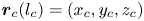 $\boldsymbol {r}_c (l_c ) = (x_c, y_c, z_c )$ specifying the coil shape. Lowercase letters and a
  $c$ subscript distinguish coil positions from positions along a magnetic field line. Here,
  $l_c$ is the arc length along the coil measured from some reference point,
  $l_c \in [0, L_c)$, where
  $L_c$ is the total coil length. The magnetic field is specified by the Biot–Savart law
 \begin{equation} \boldsymbol{B}_\textrm{coil} ={-} \sum_{c=1}^N \frac{\mu_0 I_c }{4{\rm \pi} } \int \,\textrm{d}l_c \frac{ \boldsymbol{R} - \boldsymbol{r}_c }{|\boldsymbol{R} - \boldsymbol{r}_c |^3} \times \frac{\textrm{d} \boldsymbol{r}_c}{\textrm{d}l_c} {.} \end{equation}
The poloidal gradient of the magnetic field is
 \begin{equation} \boldsymbol{\nabla}_{\boldsymbol X} \boldsymbol{B}_\textrm{coil} = \sum_{c=1}^N \frac{\mu_0 I_c }{4{\rm \pi} } \int\,\textrm{d}l_c \frac{1}{|\boldsymbol{R} - \boldsymbol{r}_c |^3 } \left[ - \textsf {I}_p + 3 \frac{ (\boldsymbol{X} - \boldsymbol{x}_c) (\boldsymbol{R} - \boldsymbol{r}_c) }{ |\boldsymbol{R} - \boldsymbol{r}_c |^2 } \right] \times \frac{\textrm{d} \boldsymbol{r}_c}{\textrm{d}l_c}, \end{equation}
where we introduce the poloidal identity matrix  $\textsf {I}_p = \hat {\boldsymbol {e}}_R \hat {\boldsymbol {e}}_R + \hat {\boldsymbol {e}}_Z \hat {\boldsymbol {e}}_Z$, with
  $\hat {\boldsymbol {e}}_Z = \boldsymbol {\nabla }_{\boldsymbol X} Z$, and the position vector of the coil projected in the poloidal plane,
  $\boldsymbol {x}_c = \boldsymbol {r}_c \boldsymbol {\cdot } ( \hat {\boldsymbol {e}}_R \hat {\boldsymbol {e}}_R + \hat {\boldsymbol {e}}_Z \hat {\boldsymbol {e}}_Z )$. The second derivative of the magnetic field is
 \begin{align} \boldsymbol{\nabla}_{\boldsymbol X} \boldsymbol{\nabla}_{\boldsymbol X} \boldsymbol{B}_\textrm{coil} &= \sum_{c=1}^N \frac{\mu_0 I_c }{4{\rm \pi} } \int\,\textrm{d}l_c \frac{1}{|\boldsymbol{R} - \boldsymbol{r}_c |^5 } \left[ 3 \left( \textsf {I}_p - 5 \frac{ (\boldsymbol{X} - \boldsymbol{x}_c) (\boldsymbol{X} - \boldsymbol{x}_c) }{ |\boldsymbol{R} - \boldsymbol{r}_c |^2 } \right) \left( \boldsymbol{R} - \boldsymbol{r}_c \right) \right. \nonumber\\ &\quad + \left. 3 \left( \boldsymbol{X} - \boldsymbol{x}_c \right) \textsf {I}_p + 3 \left( \hat{\boldsymbol{e}}_R \left( \boldsymbol{X} - \boldsymbol{x}_c \right)\hat{\boldsymbol{e}}_R + \hat{\boldsymbol{e}}_Z \left( \boldsymbol{X} - \boldsymbol{x}_c \right) \hat{\boldsymbol{e}}_Z \right) \right] \times \frac{\textrm{d} \boldsymbol{r}_c}{\textrm{d}l_c} {.} \end{align}
 The variation  $\Delta \boldsymbol {B}$ of a coil-produced magnetic field is conveniently expressed in terms of the shape gradient
  $\boldsymbol {\mathcal {G}}_{\boldsymbol {r}_c} \boldsymbol {B}$ of the magnetic field with respect to coils (Landreman & Paul Reference Landreman and Paul2018). The shape gradient
  $\boldsymbol {\mathcal {G}}_{\boldsymbol {r}_c}$ is a vector operator which, like
  $\boldsymbol {\nabla }_{\boldsymbol X}$, is meaningful only when acting on a (scalar or tensor) quantity to its right. It is defined via
 \begin{equation} \Delta f = \sum_{c=1}^N \int \,\textrm{d}l_c \left( \Delta \boldsymbol{r}_{c} \times \frac{\textrm{d} \boldsymbol{r}_c}{\textrm{d}l_c} \right) \boldsymbol{\cdot} \boldsymbol{\mathcal{G}}_{\boldsymbol{r}_c}\,f {.} \end{equation}
The shape gradient of the magnetic field can be extracted from the Biot–Savart law and (4.22) as shown in Appendix E, which gives
 \begin{equation} \boldsymbol{\mathcal{G}}_{\boldsymbol{r}_c} \boldsymbol{B}_\textrm{coil} = \frac{\mu_0 I_c }{4{\rm \pi} |\boldsymbol{R} - \boldsymbol{r}_c |^3} \left[- \textsf {I} + \frac{ 3 (\boldsymbol{R} - \boldsymbol{r}_c) \left( \boldsymbol{R} - \boldsymbol{r}_c \right) }{ |\boldsymbol{R} - \boldsymbol{r}_c |^2 } \right] , \end{equation}
where  $\textsf {I} = \hat {\boldsymbol {e}}_X \hat {\boldsymbol {e}}_X + \hat {\boldsymbol {e}}_Y \hat {\boldsymbol {e}}_Y + \hat {\boldsymbol {e}}_{Z} \hat {\boldsymbol {e}}_{Z}$.
The shape gradient of the island width with respect to the coils producing the magnetic field is
 \begin{equation} \boldsymbol{\mathcal{G}}_{\boldsymbol{r}_c} \ln w_k = \boldsymbol{\mathcal{G}}_{\boldsymbol{r}_c} \ln C - \boldsymbol{\mathcal{G}}_{\boldsymbol{r}_c} \ln \varSigma_k {.} \end{equation}
Here  $\boldsymbol {\mathcal {G}}_{\boldsymbol {r}_c} C$ is given by
 \begin{equation} \boldsymbol{\mathcal{G}}_{\boldsymbol{r}_c} C ={-} \int_0^{2{\rm \pi} L / n_0} \,\textrm{d}\varphi \boldsymbol{ \mathcal{G}}_{\boldsymbol{r}_c} \boldsymbol{V} \boldsymbol{\cdot} \boldsymbol{\lambda} , \end{equation}
with
 \begin{equation} \boldsymbol{ \mathcal{G}}_{\boldsymbol{r}_c} \boldsymbol{V} = \frac{R \boldsymbol{\mathcal{G}}_{\boldsymbol{r}_c} \boldsymbol{B}_{p} }{B_{\varphi}} - \frac{R ( \boldsymbol{\mathcal{G}}_{\boldsymbol{r}_c} B_{\varphi} ) \boldsymbol{B}_{p} }{B_{\varphi}^2 } {,} \end{equation}
and  $\boldsymbol {\mathcal {G}}_{\boldsymbol {r}_c} \varSigma _k$ is given by
 \begin{equation} \boldsymbol{\mathcal{G}}_{\boldsymbol{r}_c} \varSigma_k ={-} \sum_{Q=0}^{Q_0-1} \int_{2{\rm \pi} LQ/n_0}^{2{\rm \pi} L(Q+1)/n_0}\,\textrm{d}\varphi \left( \left( \boldsymbol{\mathcal{G}}_{\boldsymbol{r}_c} \boldsymbol{V} \right) \boldsymbol{\cdot} \boldsymbol{\lambda}_Q + \boldsymbol{s}_{{\perp} k} \boldsymbol{\cdot} \left( \boldsymbol{\nabla}_{\boldsymbol X} \boldsymbol{\mathcal{G}}_{\boldsymbol{r}_c} \boldsymbol{V} \right) \boldsymbol{\cdot} \boldsymbol{\mu} \right) , \end{equation}
with
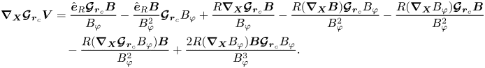 \begin{align} \boldsymbol{\nabla}_{\boldsymbol X} \boldsymbol{\mathcal{G}}_{\boldsymbol{r}_c} \boldsymbol{V} &= \frac{\hat{\boldsymbol{e}}_R \boldsymbol{\mathcal{G}}_{\boldsymbol{r}_c} \boldsymbol{B}}{B_{\varphi}} - \frac{\hat{\boldsymbol{e}}_R \boldsymbol{B}}{B_{\varphi}^2} \boldsymbol{\mathcal{G}}_{\boldsymbol{r}_c} B_{\varphi} + \frac{R \boldsymbol{\nabla}_{\boldsymbol X} \boldsymbol{\mathcal{G}}_{\boldsymbol{r}_c} \boldsymbol{B} }{B_{\varphi}} - \frac{R (\boldsymbol{\nabla}_{\boldsymbol X} \boldsymbol{B} ) \boldsymbol{\mathcal{G}}_{\boldsymbol{r}_c} B_{\varphi}}{B_{\varphi}^2} - \frac{R (\boldsymbol{\nabla}_{\boldsymbol X} B_{\varphi}) \boldsymbol{\mathcal{G}}_{\boldsymbol{r}_c} \boldsymbol{B} }{B_{\varphi}^2} \nonumber\\ &\quad - \frac{R (\boldsymbol{\nabla}_{\boldsymbol X} \boldsymbol{\mathcal{G}}_{\boldsymbol{r}_c} B_{\varphi } ) \boldsymbol{B} }{B_{\varphi}^2} + \frac{2 R (\boldsymbol{\nabla}_{\boldsymbol X} B_{\varphi } ) \boldsymbol{B} \boldsymbol{\mathcal{G}}_{\boldsymbol{r}_c} B_{\varphi} }{B_{\varphi}^3} . \end{align}
The spatial derivative (in the poloidal plane) of the shape gradient of the magnetic field is
 \begin{align} \boldsymbol{\nabla}_{\boldsymbol X} \boldsymbol{\mathcal{G}}_{\boldsymbol{r}_c} \boldsymbol{B} &= \frac{\mu_0 I_c }{4{\rm \pi} |\boldsymbol{R} - \boldsymbol{r}_c |^5} \left[ 3\left( \boldsymbol{X} - \boldsymbol{x}_c\right) \left( \textsf {I} - 5 \frac{ \left( \boldsymbol{R} - \boldsymbol{r}_c \right) \left( \boldsymbol{R} - \boldsymbol{r}_c \right) }{ |\boldsymbol{R} - \boldsymbol{r}_c |^2 } \right) \right. \nonumber\\ &\quad + \left. 3\hat{\boldsymbol{e}}_R \left( \boldsymbol{R} - \boldsymbol{r}_c \right) \hat{\boldsymbol{e}}_R + 3\hat{\boldsymbol{e}}_R \hat{\boldsymbol{e}}_R \left( \boldsymbol{R} - \boldsymbol{r}_c \right) + 3\hat{\boldsymbol{e}}_Z \left( \boldsymbol{R} - \boldsymbol{r}_c \right) \hat{\boldsymbol{e}}_Z + 3\hat{\boldsymbol{e}}_Z \hat{\boldsymbol{e}}_Z \left( \boldsymbol{R} - \boldsymbol{r}_c \right) \vphantom{\left[ 3\left( \boldsymbol{X} - \boldsymbol{x}_c\right) \left( \textsf {I} - 5 \frac{ \left( \boldsymbol{R} - \boldsymbol{r}_c \right) \left( \boldsymbol{R} - \boldsymbol{r}_c \right) }{ |\boldsymbol{R} - \boldsymbol{r}_c |^2 } \right) \right.}\right]. \end{align}
 Using these equations, a numerical approximation to the shape gradient of the width of an island in an NCSX vacuum configuration, shown in figure 4, was calculated for a type-A modular coil. The magnetic field from the toroidal field coils and from most of the poloidal field coils is included. The resonant rotational transform of the island chain is  $\iota _\textrm {res} = 1/4$. The shape gradient calculation is compared in figure 5 with a finite-difference approximation calculated by perturbing the discrete coil positions at certain locations. In figures 4 and 5, all plotted quantities are in SI units. For simplicity, in figure 5, we have plotted an alternative definition of the shape gradient
  $\overline { \boldsymbol { \mathcal {G}}_{c}} f = ( \textrm {d}\boldsymbol {r}_c / \textrm {d}l_c ) \times \boldsymbol { \mathcal {G}}_{\boldsymbol {r}_c}\,f$, which satisfies
 \begin{equation} \Delta f = \sum_{c=1}^N \int\,\textrm{d}l_c \Delta \boldsymbol{r}_{c} \boldsymbol{\cdot} \bar{\boldsymbol{\mathcal{G}}}_{\boldsymbol{r}_c}\,f {,} \end{equation}
and thus has a more intuitive geometric interpretation. In the adjoint calculation, the shape gradient is calculated by evaluating  $\boldsymbol { \mathcal {G}}_{\boldsymbol {r}_c}\,f$ using the adjoint expressions outlined in this section and a numerical approximation of
  $\textrm {d}\boldsymbol {r}_c /\textrm {d} l_c$,
 \begin{equation} \overline{\boldsymbol{\mathcal{G}}}_{\boldsymbol{r}_\textrm{c}}\,f = \frac{ \boldsymbol{r}_c ( l_c + \delta l_c ) - \boldsymbol{r}_c ( l_c - \delta l_c ) }{ 2 \delta l_c } \times \boldsymbol{\mathcal{G}}_{\boldsymbol{r}_c}\,f {,} \end{equation}
where  $\delta l_c$ is the separation between equally-spaced positions on the coil. Using a centred difference approximation instead, the components of the shape gradient,
  $\bar {\mathcal {G}}^\textrm {CD}_{\kappa _c} f$ for
  $\kappa _c \in \{ x_c, y_c, z_c \}$, are calculated from
 \begin{equation} \bar{\mathcal{G}}^\textrm{CD}_{\kappa_c} f = \frac{ f(\kappa_c + \delta \kappa_c ) - f(\kappa - \delta \kappa_c ) }{2 \delta \kappa_c \delta l_c } {.} \end{equation}
For the coil considered in this study, the centred difference shape gradient, taken with  $\delta \kappa _c = 10^{-4}$, has a good overlap with the shape gradient calculated using the adjoint method, as shown in figure 5. The direct adjoint calculation is, however, over a hundred times faster. This is because the adjoint approach requires solving a few equations along the same periodic magnetic field line, so that the magnetic field and its gradients do not need to be re-evaluated when computing the shape gradient with respect to all coil positions. Conversely, the finite-difference calculation requires searching for a new periodic field line after each finite-difference step, which is expensive because it requires re-computing the magnetic field at new locations for each coil perturbation.
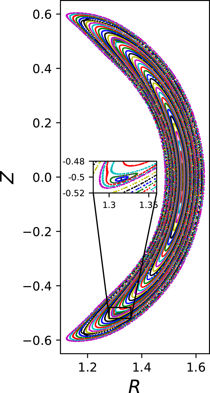


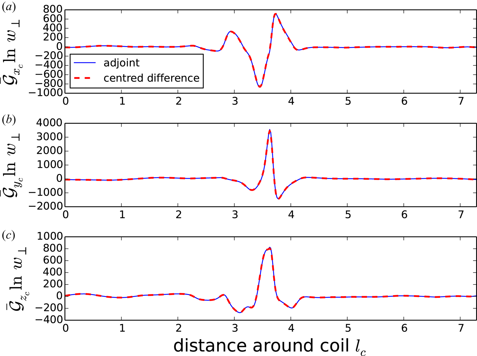
Figure 5. Shape gradient of the width of one of the magnetic islands in the NCSX configuration (figure 4) with respect to the positions along a type-A modular coil (length  $L_c = 7.29$), calculated using
  $N_{\varphi } = 30$ with: the adjoint method (solid lines); the centred difference scheme with
  $\delta \kappa _c = 10^{-4}$ (dashed lines). For each component, the mean residual between the two calculations is approximately
  $2\,\%$ of the mean absolute value. The adjoint calculation is over a hundred times faster.
4.4. Optimization of helical coils via gradient of residue
We proceed to consider a model magnetic field studied by Hanson & Cary (Reference Hanson and Cary1984), which consists of two pieces: a toroidal magnetic field generated by a long current-carrying wire passing through the centre of the torus, and a magnetic field generated by a pair of helical coils with opposite current ( $\pm I_\textrm {heli}$). The helical coil positions are specified by the poloidal angle
  $\eta _\pm$ as a function of the toroidal angle
  $\varphi$,
 \begin{equation} \eta_\pm{=} \frac{ n_0 \varphi }{l_0} + \sum_{k=0}^{k_\textrm{max}} \left[ A_{{\pm}, k} \cos \left( \frac{ kn_0 \varphi}{l_0} \right) + B_{{\pm}, k} \sin \left( \frac{ kn_0 \varphi}{l_0} \right) \right] . \end{equation}
The position of the coils  $\boldsymbol {r}_\pm = (x_\pm , y_\pm , z_\pm )$ is then obtained using the equations
 \begin{gather} x_{{\pm}} = \left( R_0 + r_0 \cos \eta_\pm \right) \cos \varphi , \end{gather}
 \begin{gather} y_\pm{=} \left( R_0 + r_0 \cos \eta_\pm \right) \sin \varphi , \end{gather}
 \begin{gather} z_\pm{=}{-} r_0 \sin \eta_\pm . \end{gather}
Here we have introduced the major and minor radius of the toroidal surface in which the helical coils lie,  $R_0$ and
  $r_0$ respectively. The magnetic field configuration is obtained by adding the toroidal magnetic field
  $\hat {\boldsymbol {e}}_{\varphi } R_0 B_t / R$ to the magnetic field obtained by applying the Biot–Savart law to the helical coils,
 \begin{equation} \boldsymbol{B}_\textrm{heli} (\boldsymbol{R}) = \frac{R_0 B_t }{ R } \hat{\boldsymbol{e}}_{\varphi} + \sum_{{\pm}} \frac{\pm \mu_0 I_\textrm{heli} }{4{\rm \pi} } \int \textrm{d}\varphi \frac{1}{ |\boldsymbol{R} - \boldsymbol{r}_{{\pm}} |^3} \frac{\textrm{d}\boldsymbol{r}_{{\pm}}}{\textrm{d}\varphi} \times (\boldsymbol{R} - \boldsymbol{r}_{{\pm}}) . \end{equation}
 Upon fixing  $R_0$,
  $r_0$,
  $I_\textrm {heli}$ and
  $B_t$, as done in Hanson & Cary (Reference Hanson and Cary1984), the continuous parameters that can be used to perturb the magnetic field configuration are
  $A_k$ for
  $0 \leqslant k \leqslant k_\textrm {max}$ and
  $B_k$ for
  $1\leqslant k \leqslant k_\textrm {max}$. Perturbing any one parameter of any one coil (carrying a current
  $\pm I_\textrm {heli}$), denoted as
  $\kappa _{\pm }$, such that the variation in the coil position is
  $\boldsymbol {r}_{\pm } (\varphi ) \rightarrow \boldsymbol {r}_{\pm } (\varphi ) + \Delta \kappa _{\pm } \partial \boldsymbol {r}_{\pm } (\varphi ) / \partial \kappa _{\pm }$, causes the magnetic field to change such that
  $\boldsymbol {B}(\boldsymbol {R}) \rightarrow \boldsymbol {B}(\boldsymbol {R}) + \Delta \kappa _{\pm } \partial \boldsymbol {B}(\boldsymbol {R}) / \partial \kappa _{\pm }$. From the expressions (4.22) and (4.23), we get
 \begin{equation} \frac{\partial \boldsymbol{B}}{\partial \kappa_{{\pm}}} ={\pm} \frac{\mu_0 I_\textrm{heli} }{4{\rm \pi}} \int \,\textrm{d}\varphi \frac{1}{|\boldsymbol{R} - \boldsymbol{r}_{{\pm}} |^3} \left[ - \textsf {I} + \frac{ 3 (\boldsymbol{R} - \boldsymbol{r}_{{\pm}}) \left( \boldsymbol{R} - \boldsymbol{r}_{{\pm}} \right) }{ |\boldsymbol{R} - \boldsymbol{r}_{{\pm}} |^2 } \right] \boldsymbol{\cdot} \left( \frac{\partial \boldsymbol{r}_{{\pm}} }{\partial \kappa } \times \frac{ \textrm{d} \boldsymbol{r}_{{\pm}} }{ \textrm{d} \varphi } \right) {.} \end{equation}
The gradient of the magnetic field changes according to  $\boldsymbol {\nabla }_{\boldsymbol X} \boldsymbol {B}(\boldsymbol {R}) \rightarrow \boldsymbol {\nabla }_{\boldsymbol X} \boldsymbol {B}(\boldsymbol {R}) + \Delta \kappa _{\pm } \partial \boldsymbol {\nabla }_{\boldsymbol X} \boldsymbol {B}(\boldsymbol {R}) / \partial \kappa _{\pm }$; from (4.22) and (4.29), we deduce
 \begin{align} \frac{\partial \boldsymbol{\nabla}_{\boldsymbol X} \boldsymbol{B}}{\partial \kappa_{{\pm}}} &={\pm} \frac{\mu_0 I_\textrm{heli} }{4{\rm \pi}} \int \textrm{d}\varphi \frac{1}{|\boldsymbol{R} - \boldsymbol{r}_{{\pm}} |^5} \left[ 3 (\boldsymbol{R} - \boldsymbol{r}_{{\pm}} ) \textsf {I} - \frac{ 5 (\boldsymbol{R} - \boldsymbol{r}_{{\pm}} ) (\boldsymbol{R} - \boldsymbol{r}_{{\pm}}) \left( \boldsymbol{R} - \boldsymbol{r}_{{\pm}} \right) }{ |\boldsymbol{R} - \boldsymbol{r}_{{\pm}} |^2 } \right. \nonumber\\ &\quad + \left. \textsf {I} \left( \boldsymbol{R} - \boldsymbol{r}_{{\pm}} \right) + \hat{\boldsymbol{e}}_R \left( \boldsymbol{R} - \boldsymbol{r}_{{\pm}} \right) \hat{\boldsymbol{e}}_R + \hat{\boldsymbol{e}}_Z \left( \boldsymbol{R} - \boldsymbol{r}_{{\pm}} \right) \hat{\boldsymbol{e}}_Z \right] \boldsymbol{\cdot} \left( \frac{\partial \boldsymbol{r}_{{\pm}} }{\partial \kappa } \times \frac{ \textrm{d} \boldsymbol{r}_{{\pm}} }{ \textrm{d} \varphi } \right) {.} \end{align}
 A gradient-based optimization scheme to demonstrate an application of the adjoint gradient formulation was performed on the system with  $R_0 = 1$,
  $r_0 = 0.3$,
  $\mu _0 I_\textrm {heli} / 4{\rm \pi} = 0.0307$ and
  $B_t = 1$. This was previously optimized by Cary & Hanson (Reference Cary and Hanson1986) using a derivative-free algorithm. The fixed parameters are
  $A_{+,0} = {\rm \pi}/{2}$,
  $A_{-,0} = A_{-,1} = B_{+,1} = 0$, and
  $A_{\pm ,k} = B_{\pm ,k} = 0$ for
  $k \geqslant 2$. The vector
  $\boldsymbol {p} = ( A_{+,1}, B_{-,1} )$ is composed of the only parameters that are varied during the optimization. Two fixed points are initially located and their residues are used in the optimization. A priori, an infinite choice of appropriate objective functions exist: the sensible properties are that they be functions of the residues of all the periodic field lines and that they be zero when all the residues are zero. The island width can only be used in the objective function if it is known that the periodic field line is an O point instead of an X point. However, periodic field lines may switch from O to X points during the optimization as
  $\boldsymbol {p}$ is varied. Moreover, the measure of island width used in this work is only accurate if the island size is small. For these reasons, using the residues in the optimization is preferable. We choose a linear combination
  $P$ of the pairs of residues,
 \begin{equation} P = \tfrac{1}{2} \left( \mathcal{R}_1 + \mathcal{R}_2 \right), \end{equation}
and we seek configurations where  $P$ is as close as possible to zero. One could, in principle, take the difference of the two residues or the mean square of the residues as the objective function: the former converges to a non-optimal solution with
  $\mathcal {R}_1 = \mathcal {R}_2$, where the objective function is zero yet the residues have not been sufficiently reduced; the latter has a much slower convergence. The function
  $|P|$ is minimized by using the gradient direction to perform a line search for solutions of
  $P = 0$, with more details discussed in Appendix F.
The initial configuration with  $\boldsymbol {p}_0 = (0.0, 0.0)$ has residues
 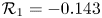 $\mathcal {R}_1 = -0.143$ and
  $\mathcal {R}_2 = 79.9$. Applying the optimization scheme, described above, results in
  $\boldsymbol {p} = (0.3414, 0.3066)$, with
  $\mathcal {R}_1 = 0.0160$ and
  $\mathcal {R}_2 = 0.0128$. The values of the parameters are similar to those obtained by Cary & Hanson (Reference Cary and Hanson1986), but give a slightly more optimized configuration: the small difference may be caused by different numerical resolutions in the Biot–Savart integral around the helical coils. The optimized and unoptimized configurations are shown in figure 6, and the helical coils that produce them are shown in figure 7. The quadratic convergence of the errors of the gradients of the residue for an intermediate step during the iteration is shown in figure 8.
Figure 6. Poincaré plots of unoptimized (a) and optimized (b) helical coil configurations. The squares indicate fixed points with residue  $\mathcal {R}_1$, while the crosses are those with residue
  $\mathcal {R}_2$.

Figure 7. Helical coils corresponding to the initial unoptimized configuration (dotted line) and to the optimized configuration (solid line). Coil  $1$ (red) carries the negative current (
 $-I_\textrm {heli}$).

Figure 8. Error convergence of the centred difference approximation of the gradient of the two residues to the adjoint calculation when  $B_{-,1} = 0.18079$ and
  $A_{+,1} = 0.25268$. The finite-difference step size on the horizontal axis is normalized to
  $\mathcal {R}^{-1} ( \partial \mathcal {R} / \partial \kappa ) \delta$ for
  $\kappa \in \lbrace A_{+,1}, B_{-,1} \rbrace$. The legend labels with respect to which parameter the gradient was taken for the different symbols, and in brackets is the value of
  $N_{\varphi }$. The higher resolution,
  $N_{\varphi } = 80$, has an increased accuracy, although the optimization is carried out at
  $N_{\varphi } = 30$ to make it faster. The decrease of the converged error for larger
  $N_{\varphi }$ indicates a discretization error in the adjoint-based approach.
5. Conclusion
In this paper, we have derived the equations for the gradients of several quantities related to magnetic islands, which include the island width and the residue of the periodic field line, using an adjoint method. The residue is a quantity that, when small and positive, is strongly correlated with island size but that can be calculated for any periodic field line, even X points in stochastic regions. Thus, although it does not quantify the physical width of an island, it is more versatile and can be used to minimize stochasticity in magnetic configurations. The gradient of the island width was obtained by differentiating the measure of island width introduced by Cary & Hanson (Reference Cary and Hanson1991). Although the island width calculation is only accurate for small islands, optimized configurations usually have small islands. Our adjoint approach thus provides an efficient and reliable method to compute the sensitivity of the island size in optimized or near-optimized stellarators.
We have performed and verified numerical gradient calculations on different magnetic field configurations. The analytical configuration of Reiman & Greenside (Reference Reiman and Greenside1986), shown in figure 1, provides the ideal system for efficiently and accurately verifying the island width calculation and the gradient calculations. Figure 2 shows a comparison of different measures of island width for this system. Figure 3 demonstrates the correct quadratic convergence of centred difference gradient approximations to the adjoint gradient calculations as the centred difference step is decreased. In figure 5, we show shape gradients of the island width with respect to a discrete set of positions along a type-A modular coil in an NCSX configuration, which highlights the overlap between the adjoint and the centred difference calculation. For NCSX, where the magnetic field evaluation is computationally expensive, a factor of over one hundred in computation time is gained by calculating the shape gradient using the adjoint method. The gradient calculation using adjoints has been successfully implemented also to a system composed of a toroidal field coil and a pair of helical coils, which were previously optimized without derivatives in Hanson & Cary (Reference Hanson and Cary1984) and Cary & Hanson (Reference Cary and Hanson1986). For one such configuration, the helical coils were optimized using the adjoint calculation of the gradient of the residue, with a result consistent with that of Cary and Hanson. The result of the optimization is shown in figure 6.
The tool we have developed in this work can be applied in several areas of stellarator design. First, shape-gradient calculations using the adjoint approach can be used to efficiently calculate coil tolerances with respect to island size in stellarator configurations. However, they can also be used in optimization, as demonstrated in § 4.4. Gradient-based minimization of stochasticity and island size, as well as optimization of island width sensitivity, are possible applications of this work.
Acknowledgements
The authors would like to thank A. Cerfon for suggesting to use of the Reiman model as a test magnetic field configuration. A.G. would like like to thank C. Smiet and M. Sadr for stimulating and useful discussions. This work was supported by the US Department of Energy through grant DE-FG02-93ER-54197.
Editor P. Helander thanks the referees for their advice in evaluating this article.
Declaration of interests
The authors report no conflict of interest.
Appendix A. Magnetic field line trajectory as a Hamiltonian system
A fundamental property of the magnetic field, namely that it is divergenceless, is imposed by defining  $\boldsymbol {B}$ as the curl of a vector potential,
 \begin{equation} \boldsymbol{B} = \boldsymbol{\nabla} \times \boldsymbol{A} . \end{equation}
Note that  $\boldsymbol {A}$ is not uniquely defined: adding the gradient of a scalar function,
  $\boldsymbol {\nabla } g$, called a gauge transformation, leaves
  $\boldsymbol {B}$ unchanged. The form of
  $\boldsymbol {B}$ we have adopted in (2.1) corresponds to the vector potential
 \begin{equation} \boldsymbol{A} = \psi \boldsymbol{\nabla} \theta - \chi (\psi, \theta, \varphi ) \boldsymbol{\nabla} \varphi , \end{equation}
where we have chosen a particular gauge.
Considering  $\boldsymbol {R} (\varphi )$ as the position vector following a field line, (A 1) can be derived by extremizing the action
 \begin{equation} S = \int_{\varphi_1}^{\varphi_2} \mathcal{L} \left( \boldsymbol{R}(\varphi), \varphi \right) \,\textrm{d}\varphi \end{equation}
with respect to  $\boldsymbol {R}(\varphi )$, where the end-points along the path,
  $\boldsymbol {R} ( \varphi _1 )$ and
  $\boldsymbol {R} ( \varphi _2 )$, are fixed, and the Lagrangian
  $\mathcal {L}$ is
 \begin{equation} \mathcal{L} = \boldsymbol{A} (\boldsymbol{R}) \boldsymbol{\cdot} \frac{\textrm{d}\boldsymbol{R}}{\textrm{d}\varphi} . \end{equation}
The choice (A 4) can be verified using the Euler–Lagrange equation resulting from the extremization of the action,
 \begin{equation} \frac{\textrm{d}}{\textrm{d}\varphi} \left( \frac{\textrm{d}\mathcal{L}}{\partial \dot{\boldsymbol{R}}} \right) = \frac{\textrm{d}\mathcal{L}}{\partial \boldsymbol{R}} , \end{equation}
which leads to the equation  $\boldsymbol {B} \times \textrm {d}\boldsymbol {R} / \textrm {d}\varphi = 0$, and implies that
  $\textrm {d}\boldsymbol {R} / \textrm {d}\varphi$ is always parallel to
  $\boldsymbol {B}$. Upon inserting (A 2) into (A 4), the action
  $S$ in (A 3) becomes
 \begin{equation} S = \int_{\varphi_1}^{\varphi_2} \left( \psi \frac{\textrm{d} \theta}{\textrm{d}\varphi} - \chi (\psi, \theta, \varphi) \right)\,\textrm{d}\varphi. \end{equation}
The action expressed in the form (A 6) can be directly compared with the standard form for the action of a Hamiltonian system,
 \begin{equation} S = \int_{t_1}^{t_2} \left( p \frac{\textrm{d}q}{\textrm{d}t} - H (q, p, t) \right) \,\textrm{d}t. \end{equation}
Hence, it follows that the trajectory of a magnetic field line as a function of toroidal angle constitutes a Hamiltonian system where the canonical coordinate  $q$ is
  $\theta$, the canonical momentum
  $p$ is
  $\psi$, the Hamiltonian
  $H$ is
  $\chi$ and the time
  $t$ is
  $\varphi$.
A.1. Hamiltonian after replacing $\theta$ with $\varTheta$


We proceed to obtain the Hamiltonian after the change of variables  $(\theta , \psi ) \rightarrow (\varTheta , \psi )$, where
  $\varTheta = \theta - \iota _0(\psi _0) \varphi$ is the poloidal angle relative to the unperturbed magnetic field line at the flux surface
  $\psi = \psi _0$ crossing
  $\varphi = \theta = 0$. To this end, we re-express
  $\textrm {d}\theta / \textrm {d}\varphi$ by applying the chain rule to the equation
  $\theta = \varTheta + \iota _0 (\psi _0) \varphi$,
 \begin{equation} \frac{\textrm{d}\theta}{\textrm{d}\varphi} = \left( \frac{\partial \theta }{\partial \varTheta } \right)_{\varphi} \frac{\textrm{d}\varTheta}{\textrm{d}\varphi} + \left( \frac{\partial \theta}{\partial \varphi} \right)_{\varTheta} = \frac{\textrm{d}\varTheta}{\textrm{d}\varphi} + \iota_0 ( \psi_0 ). \end{equation}
Here, a subscript to the right of the parentheses indicates what variable is being kept constant in the partial differentiation within the parentheses. By using (A 8), the action in (A 6) becomes
 \begin{equation} S = \int_{\varphi_1}^{\varphi_2} \left( \psi \frac{\textrm{d}\varTheta}{ \textrm{d}\varphi } + \psi \iota_0 (\psi_0) - \chi (\psi, \varTheta ) \right) \,\textrm{d}\varphi. \end{equation}
Therefore, the Hamiltonian  $K$ in the new variables is given by (2.10). This is effectively the result of a canonical transformation involving the independent variable (Goldstein, Poole & Safko Reference Goldstein, Poole and Safko2002).
Appendix B. Dominance of resonant perturbation
The equations of the magnetic field line trajectory including the perturbation are
 \begin{equation} \frac{\textrm{d}\theta }{\textrm{d}\varphi} = \iota_0(\psi) + \sum_{m,n} \chi_{m,n}'(\psi) \exp \left( \textrm{i}m\theta - \textrm{i}n \varphi \right) {,} \end{equation}
and
 \begin{equation} \frac{\textrm{d}\psi }{\textrm{d}\varphi} ={-} \sum_{m,n} \chi_{m,n}(\psi) \textrm{i}m\exp \left( \textrm{i}m\theta - \textrm{i}n \varphi \right) {.} \end{equation}
The solutions of (B 1) and (B 2) are assumed to be approximately given by the functions obtained from (2.3)–(2.4),
 \begin{equation} \psi \simeq \psi_0 + \psi_1 (\varphi) {,} \end{equation}
and
 \begin{equation} \theta \simeq \theta_{\text{i}} + \iota_0 (\psi_0) \varphi + \theta_1 (\varphi) {,} \end{equation}
where  $\psi _1$ and
  $\theta _1$ are additional functions – assumed small – that depend on the perturbation, and
  $\theta _\textrm {i}$ is the value of
  $\theta$ at
  $\varphi = 0$. Because
  $|\chi _1 | \ll \chi _0$, we assume that
  $\psi \simeq \psi _0$ so that
  $\psi _1$ and
  $\theta _1$ are small corrections, and calculate
  $\theta _1$ by neglecting it in the phase of the perturbation,
 \begin{equation} \frac{\textrm{d}\theta_1 }{\textrm{d}\varphi} \simeq \sum_{m,n} \chi_{m,n}'(\psi_0) \exp \left( \textrm{i}m \theta_{\text{i}} + \textrm{i}m \iota_0 \varphi - \textrm{i}n \varphi \right) {.} \end{equation}
This gives
 \begin{equation} \theta_1 \simeq \sum_{m,n} \frac{ \chi_{m,n}'(\psi_0) }{ \textrm{i}m \iota_0 - \textrm{i} n} \exp \left( \textrm{i}m\theta_{\text{i}} + \textrm{i}m \iota_0 \varphi - \textrm{i}n \varphi \right) {,} \end{equation}
which is divergent when  $n/m = \iota _0$. Hence, we deduce that the effect of the perturbation is dominated by the Fourier modes that coincide (resonate) with the rotational transform of the unperturbed flux surface,
  $n/m = \iota _0$.
Appendix C. Variation of periodic field line position
The periodic field line position changes owing to the variation of the magnetic field configuration, which affects the circumference and in turn the island width, as discussed in § 2. However, the gradient of the poloidal position vector  $\bar {\boldsymbol {X}}_k$ is itself useful to search faster and more reliably for the new position of the periodic field line after a small change in parameters, e.g. during the optimization considered in § 4.4. We thus proceed to derive the variation
  $\Delta \bar {\boldsymbol {X}}_k$.
We introduce the vector Lagrangian
 \begin{equation} \mathcal{L}_{\bar{\boldsymbol{X}}} = \bar{\boldsymbol{X}}_k + \int_{2{\rm \pi} k/n_0}^{2{\rm \pi} (k+L)/n_0} \left( \frac{\textrm{d}\boldsymbol{X}}{\textrm{d}\varphi} - \boldsymbol{V} \right) \boldsymbol{\cdot} \mu_{\bar{\boldsymbol{X}}_k} \textrm{d}\varphi {.} \end{equation}
In (3.30), we have introduced a constraint using the adjoint variable  $\boldsymbol {\mu }_{\bar {\boldsymbol {X}}_k}$ (a matrix). Extremization with respect to variations in
  $\boldsymbol {X} (\varphi )$ gives
 \begin{align} \Delta \mathcal{L}_{\bar{\boldsymbol{X}}} &= \Delta \bar{\boldsymbol{X}}_k + \int_{2{\rm \pi} k/n_0}^{2{\rm \pi} (k+L)/n_0} \Delta \boldsymbol{X} \boldsymbol{\cdot} \left( -\frac{\textrm{d}\boldsymbol{\mu}_{\boldsymbol{X}_k}}{\textrm{d}\varphi} - \boldsymbol{\nabla}_{\boldsymbol X} \boldsymbol{V} \boldsymbol{\cdot} \boldsymbol{\mu}_{\bar{\boldsymbol{X}}_k} \right) \,\textrm{d}\varphi\nonumber\\ &\quad + \Delta \boldsymbol{X} \left( 2{\rm \pi} (k+L)/n_0 \right) \boldsymbol{\cdot} \boldsymbol{\mu}_{\bar{\boldsymbol{X}}_k} \left( 2{\rm \pi} (k+L)/n_0 \right)\notag\\ &\quad - \Delta \boldsymbol{X} \left( 2{\rm \pi} k / n_0 \right) \boldsymbol{\cdot} \boldsymbol{\mu}_{\bar{\boldsymbol{X}}_k} \left( 2{\rm \pi} k / n_0 ) \right) \text{.} \end{align}
Considering  $\Delta \boldsymbol {X} ( 2{\rm \pi} (k+L)/n_0 ) = \Delta \boldsymbol {X} ( 2{\rm \pi} k/n_0 ) = \Delta \bar {\boldsymbol {X}}_k$, the adjoint equation is
 \begin{equation} \frac{\textrm{d}\boldsymbol{\mu}_{\bar{\boldsymbol{X}}_k}}{\textrm{d}\varphi} ={-} \boldsymbol{\nabla}_{\bar{\boldsymbol{X}}} \boldsymbol{V} \boldsymbol{\cdot} \boldsymbol{\mu}_{\bar{\boldsymbol{X}}_k} , \end{equation}
and must be solved with the boundary condition  $\boldsymbol {\mu }_{\bar {\boldsymbol {X}}_k} ( 2{\rm \pi} (k+L)/n_0 ) = \boldsymbol {\mu }_{\bar {\boldsymbol {X}}_k} ( 2{\rm \pi} k/ n_0 ) - \textsf {I}$.
The boundary condition can be simplified as follows. The transpose of (2.46) is
 \begin{equation} \frac{\textrm{d}\textsf {S}_k^\intercal}{\textrm{d}\varphi} = \textsf {S}_k^\intercal \boldsymbol{\cdot} \boldsymbol{\nabla}_{\boldsymbol X} \boldsymbol{V} . \end{equation}
Premultiplying and postmultiplying by the adjoint of  $\textsf {S}_k$,
  $\textsf {S}_k^{{\dagger} } = ( \textsf {S}_k^\intercal )^{-1}$, and noting that
  $\textsf {S}_k^{{\dagger} } \boldsymbol {\cdot } \textrm {d}\textsf {S}_k^{\intercal } / \textrm {d}\varphi = - ( \textrm {d}\textsf {S}_k^{{\dagger} } / \textrm {d}\varphi ) \boldsymbol {\cdot } \textsf {S}_k^\intercal$ (from the chain rule and
  $\textsf {S}_k^{{\dagger} } \boldsymbol {\cdot } \textsf {S}_k^\intercal = \textsf {I}$), results in
 \begin{equation} \frac{\textrm{d} \textsf {S}_k^{{{\dagger}}}}{\textrm{d}\varphi} ={-} \boldsymbol{\nabla}_{\boldsymbol X} \boldsymbol{V} \boldsymbol{\cdot} \textsf {S}_k^{{{\dagger}}} . \end{equation}
Comparing (C 3) and (C 5), and using  $\textsf {S}_k ( 2{\rm \pi} (k + L) / n_0 )= \textsf {M}_k$ with
 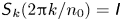 $\textsf {S}_k ( 2{\rm \pi} k / n_0 )= \textsf {I}$, gives
 \begin{equation} \boldsymbol{\mu}_{\bar{\boldsymbol{X}}_k} \left( 2{\rm \pi} (k + L) /n_0 \right) = \textsf {M}_k^{{{\dagger}}} \boldsymbol{\cdot} \boldsymbol{\mu}_{\bar{\boldsymbol{X}}} \left( 2{\rm \pi} k/n_0 \right) . \end{equation}
Hence, the appropriate boundary condition for (C 3) is
 \begin{equation} \boldsymbol{\mu}_{\bar{\boldsymbol{X}}_k}(2{\rm \pi} k / n_0) = \left[ \textsf {I} - \textsf {M}_k^{{{\dagger}}} \right]^{{-}1} . \end{equation}
The variation of  $\bar {\boldsymbol {X}}_k$ is then given by
 \begin{equation} \Delta \bar{\boldsymbol{X}}_k ={-} \int_{2{\rm \pi} k/n_0}^{2{\rm \pi} (k+L)/n_0} \Delta \boldsymbol{V} \boldsymbol{\cdot} \boldsymbol{\mu}_{\bar{\boldsymbol{X}}_k} \,\textrm{d}\varphi . \end{equation}
Appendix D. Formulae for the Reiman magnetic field configuration
The analytical magnetic field configuration is adapted from a model magnetic field used in Reiman & Greenside (Reference Reiman and Greenside1986). The magnetic field components are, from (2.1) and (4.3)–(4.6),
 \begin{gather} B_R = \frac{Z}{R} D_0 + \frac{R-R_0}{ R} D_1 {,} \end{gather}
 \begin{gather}B_Z ={-} \frac{R-R_0}{R} D_0 + \frac{Z}{ R} D_1 {,} \end{gather}
 \begin{gather}B_{\varphi} ={-} 1 {,} \end{gather}
where
 \begin{gather} D_0 = \iota_\textrm{ax} + \iota'_\textrm{ax} r^2 - \sum_{k=1}^{k_\textrm{max}} k \varepsilon_k r^{k-2} \cos \left( k \theta - \varphi \right) {,} \end{gather}
 \begin{gather}D_1 = \sum_{k=1}^{k_\textrm{max}} k \varepsilon_k r^{k-2} \sin \left( k \theta - \varphi \right) {.} \end{gather}
From (D 1)–(D 3), the gradients of the magnetic field components with respect to the poloidal coordinates  $R$ and
  $Z$ are
 \begin{gather} \partial_R B_R ={-} \frac{Z}{R^2} D_0 + \frac{Z}{R} \partial_R D_0 + \frac{R_0}{ R^2} D_1 + \frac{R-R_0}{ R} \partial_R D_1 {,} \end{gather}
 \begin{gather}\partial_Z B_R = \frac{1}{R} D_0 + \frac{Z}{R} \partial_Z D_0 + \frac{R-R_0}{ R} \partial_Z D_1 {,} \end{gather}
 \begin{gather}\partial_R B_Z ={-} \frac{R_0}{R^2} D_0 - \frac{R-R_0}{R} \partial_R D_0 - \frac{Z}{ R^2} D_1 + \frac{Z}{ R} \partial_R D_1 {,} \end{gather}
 \begin{gather}\partial_Z B_Z ={-} \frac{R-R_0}{R} \partial_Z D_0 + \frac{1}{ R} D_1 + \frac{Z}{ R} \partial_Z D_1 {,} \end{gather}
 \begin{gather}\partial_R B_{\varphi} = \partial_Z B_{\varphi} = 0 {,} \end{gather}
where
 \begin{gather} \partial_R D_0 = 2 \iota'_\textrm{ax} \left( R - R_0 \right) - \sum_{k=1}^{k_\textrm{max}} k \varepsilon_k r^{k-4} \left( \left( k - 2 \right) \left(R-R_0 \right) \cos \left( k \theta - \varphi \right) + kZ \sin \left( k \theta - \varphi \right) \right) {,} \end{gather}
 \begin{gather}\partial_R D_1 = \sum_{k=1}^{k_\textrm{max}} k \varepsilon_k r^{k-4} \left( \left( k - 2 \right) \left( R - R_0 \right) \sin \left( k \theta - \varphi \right) - kZ \cos \left( k \theta - \varphi \right) \right) {,} \end{gather}
 \begin{gather}\partial_Z D_0 = 2 \iota'_\textrm{ax} Z - \sum_{k=1}^{k_\textrm{max}} k \varepsilon_k r^{k-4} \left( \left( k - 2 \right) Z \cos \left( k \theta - \varphi \right) - k\left( R-R_0 \right) \sin \left( k \theta - \varphi \right) \right) {,} \end{gather}
 \begin{gather}\partial_Z D_1 = \sum_{k=1}^{k_\textrm{max}} k \varepsilon_k r^{k-4} \left( \left( k - 2 \right) Z \sin \left( k \theta - \varphi \right) + k \left(R-R_0 \right) \cos \left( k \theta - \varphi \right) \right) {.} \end{gather}
From (D 6)–(D 10), the second derivatives of the magnetic field components with respect to  $R$ and
  $Z$ are
 \begin{gather} \partial_{RR} B_R = \frac{2Z}{R^3} D_0 - \frac{2R_0}{ R^3} D_1 - \frac{2Z}{R^2} \partial_R D_0 + \frac{2R_0}{ R^2} \partial_R D_1 + \frac{Z}{R} \partial_{RR}D_0 + \frac{R-R_0}{ R} \partial_{RR} D_1 {,} \end{gather}
 \begin{gather}\partial_{RZ} B_R ={-} \frac{1}{R^2} D_0 - \frac{Z}{R^2} \partial_Z D_0 + \frac{1}{ R} \partial_R D_0 + \frac{R_0}{R^2} \partial_Z D_1 + \frac{Z}{ R} \partial_{RZ} D_0 + \frac{R-R_0}{R} \partial_{RZ} D_1 {,} \end{gather}
 \begin{gather}\partial_{ZZ} B_R = \frac{2}{R} \partial_{Z} D_0 + \frac{Z}{R} \partial_{ZZ} D_0 + \frac{R-R_0}{R} \partial_{ZZ} D_1, \end{gather}
 \begin{gather}\partial_{RR} B_Z = \frac{2R_0}{R^3} D_0 + \frac{2Z}{R^3} D_1 - \frac{2R_0}{R^2} \partial_R D_0 - \frac{2Z}{R^2} \partial_R D_1 - \frac{R-R_0}{R} \partial_{RR} D_0 + \frac{Z}{ R} \partial_{RR} D_1 {,} \end{gather}
 \begin{gather}\partial_{RZ} B_Z ={-} \frac{1}{R^2} D_1 - \frac{R_0}{R^2} \partial_Z D_0 - \frac{Z}{ R^2} \partial_Z D_1 + \frac{1}{R} \partial_R D_1 - \frac{R-R_0}{ R} \partial_{RZ} D_0 + \frac{Z}{ R} \partial_{RZ} D_1 {,} \end{gather}
 \begin{gather}\partial_{ZZ} B_Z = \frac{2}{R} \partial_Z D_1 - \frac{R-R_0}{ R} \partial_{ZZ} D_0 + \frac{Z}{ R} \partial_{ZZ} D_1 {,} \end{gather}
 \begin{gather}\partial_{RR} B_{\varphi} = \partial_{RZ} B_{\varphi} = \partial_{ZZ} B_{\varphi} = 0 {,} \end{gather}
where  $\partial _{RZ} = \partial _{ZR}$ and
 \begin{gather} \partial_{RR} D_0 = 2 \iota'_\textrm{ax} - \sum_{k=1}^{k_\textrm{max}} k \varepsilon_k r^{k-6} \left[ \left( \left( k - 2 \right) \left( r^2 + (k-4)(R-R_0)^2 \right) - k^2 Z^2 \right) \cos \left( k \theta - \varphi \right) \right. \nonumber\\ + \left. kZ (R - R_0 ) (2k - 6) \sin \left( k \theta - \varphi \right) \right]{,} \end{gather}
 \begin{gather} \partial_{RZ} D_0 ={-} \sum_{k=1}^{k_\textrm{max}} k \varepsilon_k r^{k-6} \left[ k \left( r^2 - (k-2)(R-R_0)^2 + (k-4)Z^2 \right) \sin \left( k \theta - \varphi \right) \right. \nonumber\\ + \left. kZ (R - R_0 ) (2k^2 - 6k + 8) \cos \left( k \theta - \varphi \right) \right] {,} \end{gather}
 \begin{gather} \partial_{ZZ} D_0 = 2 \iota'_\textrm{ax} - \sum_{k=1}^{k_\textrm{max}} k \varepsilon_k r^{k-6} \left[ \left( \left( k - 2 \right) \left( r^2 + (k-4)Z^2 \right) - k^2 (R-R_0)^2 \right) \cos \left( k \theta - \varphi \right) \right. \nonumber\\ - \left. kZ (R - R_0 ) (2k - 6) \sin \left( k \theta - \varphi \right) \right] {,} \end{gather}
 \begin{gather} \partial_{RR} D_1 = \sum_{k=1}^{k_\textrm{max}} k \varepsilon_k r^{k-6} \left[ \left( \left( k - 2 \right) \left( r^2 + (k-4)(R-R_0)^2 \right) - k^2 Z^2 \right) \sin \left( k \theta - \varphi \right) \right. \nonumber\\ - \left. kZ(R - R_0 ) \left( 2k-6 \right) \cos \left( k \theta - \varphi \right) \right]{,} \end{gather}
 \begin{gather} \partial_{RZ} D_1 = \sum_{k=1}^{k_\textrm{max}} k \varepsilon_k r^{k-6} \left[ k \left( - r^2 + (k-2)(R-R_0)^2 - (k-4)Z^2 \right) \cos \left( k \theta - \varphi \right) \right. \nonumber\\ + \left. kZ (R - R_0 ) (2k^2 - 6k + 8) \sin \left( k \theta - \varphi \right) \right] {,} \end{gather}
 \begin{gather} \partial_{ZZ} D_1 = \sum_{k=1}^{k_\textrm{max}} k \varepsilon_k r^{k-6} \left[ \left( \left( k - 2 \right) \left( r^2 + (k-4)Z^2 \right) - k^2 (R-R_0)^2 \right) \sin \left( k \theta - \varphi \right) \right. \notag\\ + \left. kZ (R - R_0 ) (2k - 6) \cos \left( k \theta - \varphi \right) \right] {.} \end{gather}
All the equations in this appendix are linear in the parameters  $\kappa \in (\iota _\textrm {ax}, \iota '_\textrm {ax}, \varepsilon )$. Hence, the gradients of the magnetic field and its first poloidal derivatives can be straightforwardly extracted.
Appendix E. Shape gradient of coil-produced magnetic field
The magnetic field produced by a set of  $N$ coils, indexed
  $c$, is given by the Biot–Savart law (4.19). Perturbing the coils, such that
  $\boldsymbol {r}_c (l_c ) \rightarrow \boldsymbol {r}_c (l_c ) + \Delta \boldsymbol {r}_c (l_c )$, changes the magnetic field, such that
  $\boldsymbol {B}(\boldsymbol {R}) \rightarrow \boldsymbol {B}(\boldsymbol {R}) + \Delta \boldsymbol {B}(\boldsymbol {R})$, where the change in magnetic field is given by
 \begin{align} \Delta \boldsymbol{B}_\textrm{coil} = -\sum_{c=1}^N \frac{\mu_0 I_c }{4{\rm \pi}} \oint\, \textrm{d}l_c \left( \Delta \boldsymbol{r}_c \boldsymbol{\cdot} \boldsymbol{\nabla}_{\boldsymbol{r}_c} \left( \frac{\boldsymbol{R} - \boldsymbol{r}_c}{ | \boldsymbol{R} - \boldsymbol{r}_c |^3 } \right) \times \frac{\textrm{d}\boldsymbol{r}_c}{\textrm{d}l_c} + \left( \frac{\boldsymbol{R} - \boldsymbol{r}_c}{ | \boldsymbol{R} - \boldsymbol{r}_c |^3 } \right) \times \frac{d\Delta \boldsymbol{r}_c}{\textrm{d}l_c} \right) {.} \end{align}
where
 \begin{equation} \boldsymbol{\nabla}_{\boldsymbol{r}_c} \left( \frac{\boldsymbol{R} - \boldsymbol{r}_c}{ | \boldsymbol{R} - \boldsymbol{r}_c |^3 } \right) = \frac{1}{ | \boldsymbol{R} - \boldsymbol{r}_c |^3 } \left( - \textsf {I} + \frac{ 3\left( \boldsymbol{R} - \boldsymbol{r}_c \right) \left( \boldsymbol{R} - \boldsymbol{r}_c \right) }{ | \boldsymbol{R} - \boldsymbol{r}_c |^3 } \right) {.} \end{equation}
An important property of (E 2) is that
 \begin{equation} \textrm{Tr} \left[ \boldsymbol{\nabla}_{\boldsymbol{r}_c} \left( \frac{\boldsymbol{R} - \boldsymbol{r}_c}{ | \boldsymbol{R} - \boldsymbol{r}_c |^3 } \right) \right] = 0 . \end{equation}
The second term in (E 1) can be re-expressed using integration by parts as
 \begin{equation} \oint\, \textrm{d}l_c \left( \frac{\boldsymbol{R} - \boldsymbol{r}_c}{ | \boldsymbol{R} - \boldsymbol{r}_c |^3 } \right) \times \frac{\textrm{d} \Delta \boldsymbol{r}_c}{\textrm{d}l_c} ={-} \oint\, \textrm{d}l_c \frac{\textrm{d}\boldsymbol{r}_c}{\textrm{d}l_c} \boldsymbol{\cdot} \boldsymbol{\nabla}_{\boldsymbol{r}_c} \left( \frac{\boldsymbol{R} - \boldsymbol{r}_c}{ | \boldsymbol{R} - \boldsymbol{r}_c |^3 } \right) \times \Delta \boldsymbol{r}_c {,} \end{equation}
where the term involving an integral of a total derivative has vanished owing to the integral being periodic. Inserting this into the previous equation gives
 \begin{equation} \Delta \boldsymbol{B}_\textrm{coil} = - \sum_{c=1}^N \frac{\mu_0 I_c }{4{\rm \pi}} \oint \,\textrm{d}l_c \left( \Delta \boldsymbol{r}_c \boldsymbol{\cdot} \boldsymbol{\nabla}_{\boldsymbol{r}_c} \left( \frac{\boldsymbol{R} - \boldsymbol{r}_c}{ | \boldsymbol{R} - \boldsymbol{r}_c |^3 } \right) \times \frac{\textrm{d} \boldsymbol{r}_c}{\,\textrm{d}l_c} - \frac{\textrm{d} \boldsymbol{r}_c}{\textrm{d}l_c} \boldsymbol{\cdot} \boldsymbol{\nabla}_{\boldsymbol{r}_c} \left( \frac{\boldsymbol{R} - \boldsymbol{r}_c}{ | \boldsymbol{R} - \boldsymbol{r}_c |^3 } \right) \times \Delta \boldsymbol{r}_c \right) {.} \end{equation}
It is an exercise in vector identities to show that
 \begin{align} &\Delta \boldsymbol{r}_c \boldsymbol{\cdot} \boldsymbol{\nabla}_{\boldsymbol{r}_c} \left( \frac{\boldsymbol{R} - \boldsymbol{r}_c}{ | \boldsymbol{R} - \boldsymbol{r}_c |^3 } \right) \times \frac{\textrm{d} \boldsymbol{r}_c}{\textrm{d}l_c} - \frac{\textrm{d} \boldsymbol{r}_c}{\textrm{d}l_c} \boldsymbol{\cdot} \boldsymbol{\nabla}_{\boldsymbol{r}_c} \left( \frac{\boldsymbol{R} - \boldsymbol{r}_c}{ | \boldsymbol{R} - \boldsymbol{r}_c |^3 } \right) \times \Delta \boldsymbol{r}_c \nonumber\\ &\quad = \textrm{Tr} \left[ \boldsymbol{\nabla}_{\boldsymbol{r}_c} \left( \frac{\boldsymbol{R} - \boldsymbol{r}_c}{ | \boldsymbol{R} - \boldsymbol{r}_c |^3 } \right) \right] \Delta \boldsymbol{r}_c \times \frac{\textrm{d} \boldsymbol{r}_c}{\textrm{d}l_c} - \boldsymbol{\nabla}_{\boldsymbol{r}_c} \left( \frac{\boldsymbol{R} - \boldsymbol{r}_c}{ | \boldsymbol{R} - \boldsymbol{r}_c |^3 } \right) \boldsymbol{\cdot} \Delta \boldsymbol{r}_c \times \frac{\textrm{d} \boldsymbol{r}_c}{\textrm{d}l_c} . \end{align}
Using (E 3), the first term on the right-hand side of (E 6) vanishes. Inserting (E 2), (E 3) and (E 6) into (E 5) gives (4.23) for the shape gradient.
Appendix F. Optimization scheme
The iteration scheme used to search for solutions of  $P = 0$ exploits the direction vector
  $\boldsymbol {d}_n$ obtained from the gradient of
  $P_n$ with respect to the two variable parameters,
 \begin{equation} \boldsymbol{d}_{n} = \left( \frac{\partial P_n}{ \partial A_{+,1} } , \frac{ \partial P_n}{ \partial B_{-,1} } \right). \end{equation}
Here, a subscript  $n$ denotes the value of the quantity at the
  $n$th step in the iteration. Starting from an initial guess
  $\boldsymbol {p}_0 = (0.0, 0.0)$, the next step in the iteration is tentatively specified by
 \begin{equation} \boldsymbol{p}_{n+1} = \boldsymbol{p}_n + \boldsymbol{p}_{n, {\rm step}} , \end{equation}
where
 \begin{equation} \boldsymbol{p}_{n, {\rm step}} ={-} \frac{g_{n}}{2^r} \frac{ P_{n} \boldsymbol{d}_n}{|\boldsymbol{d}_n|^2} \rm , \end{equation}
and where  $g_{n} > 0$ is a number chosen at each iteration and
  $r$ is the number of times the move (F 2) is rejected at a particular iteration. The reference value of
  $g_n$ is denoted
  $\bar {g}_n$ and is specified as follows. Initially, we set
  $\bar {g}_0 = 1$. Then, if at any particular iteration the number of times
  $r$ the move (F 2) gets rejected before being accepted exceeds a threshold value
  $r_\textrm {limit} = 3$, we set
  $\bar {g}_{n+1} = \bar {g}_{n} / 2$, otherwise we keep the reference value unchanged,
  $\bar {g}_{n+1} = \bar {g}_{n}$. The move (F 2) is rejected if the step in parameter space leads to an increase in the absolute value of the objective function,
  $| P_{n+1} | \geqslant | P_n|$.
There is an additional rejection criterion that is linked to a maximum value of the step in the fixed-point position,  $| \bar {\boldsymbol {X}}^{n+1} - \bar {\boldsymbol {X}}^{n} |$ (the subscript labelling the fixed point is omitted to avoid clutter, and the superscript is the iteration step number). This is necessary to ensure that the iteration proceeds successfully. At the iteration step
  $n+1$, the scheme to search for a periodic field line is applied with the initial guess equal to
  $\bar {\boldsymbol {X}}^{n} - \boldsymbol p_{n,{\rm step}} \boldsymbol {\cdot } \boldsymbol {\nabla }_{\boldsymbol {p}} \bar {\boldsymbol {X}}^n$. The gradient of the fixed-point position with respect to the parameters,
  $\boldsymbol {\nabla }_{\boldsymbol {p}} \bar {\boldsymbol {X}}^n = \partial \bar {\boldsymbol {X}}^n / \partial \boldsymbol {p}$, is calculated from the equations of Appendix C. A common way for the search for the new fixed-point position
  $\boldsymbol {X}^{n+1}$ to fail is by returning the magnetic axis (which is always a periodic solution of the magnetic field line equations for any toroidal interval that is a multiple of the the field periodicity). To avoid this, the maximum step size is set to be a fraction
  $u$ of the smallest distance between the fixed point and the magnetic axis
  $| \bar {\boldsymbol {X}}^{n} - \bar {\boldsymbol {X}}_\textrm {axis}^{n} |$. The value
  $u = 0.3$ was used.
To summarize, the criterion for accepting or rejecting a step (F 2) is:
 \begin{equation} \left. \begin{gathered} \text{accept move if } \left| P_{n+1} \right| < \left| P_n \right| \text{ and } |\bar{\boldsymbol{X}}^{n+1} - \bar{\boldsymbol{X}}^{n} | < u \left| \bar{\boldsymbol{X}}^{ n} - \bar{\boldsymbol{X}}_\textrm{axis}^n \right| {;} \\ \text{reject move if } \left| P_{n+1} \right| \geqslant \left| P_n \right| \text{ or } |\bar{\boldsymbol{X}}^{n+1} - \bar{\boldsymbol{X}}^{n} | \geqslant u \left| \bar{\boldsymbol{X}}^{ n} - \bar{\boldsymbol{X}}_\textrm{axis}^n \right| {.} \end{gathered} \right\} \end{equation}
Once a move (F 2) is accepted, it becomes permanent and the following move  $\boldsymbol {p}_{n+1, {\rm step}}$ is calculated. The optimization is stopped when
  $| P_{n-1} - P_n | < 10^{-12}$.


 Open access