


1. Introduction
A complex flow field can be modelled as a collection of flux tubes, such as hydrodynamic flows (Moffatt & Tsinober Reference Moffatt and Tsinober1992; Kleckner & Irvine Reference Kleckner and Irvine2013), superfluids (Koplik & Levine Reference Koplik and Levine1996; Kleckner, Kauffman & Irvine Reference Kleckner, Kauffman and Irvine2016) and plasmas (Cirtain et al. Reference Cirtain2013). In particular, the vortex tube is a candidate elementary structure of turbulence (Hussain Reference Hussain1986; Moffatt, Kida & Ohkitani Reference Moffatt, Kida and Ohkitani1994; Pullin & Saffman Reference Pullin and Saffman1998) (see figure 1a). Prototypical examples include rings in jets and wakes, and ‘typical eddies’ in turbulent boundary layers (Robinson Reference Robinson1991). Vortex line coiling within a vortex tube – a topological manifestation of the helicity (Moffatt Reference Moffatt1969; Moffatt & Ricca Reference Moffatt and Ricca1992) – plays an essential role in flow evolution, such as laminar–turbulence transition (Fritts, Arendt & Andreassen Reference Fritts, Arendt and Andreassen1998; Ruan et al. Reference Ruan, Xiong, You and Yang2022), vortex instability (Mayer & Powell Reference Mayer and Powell1992; Pradeep & Hussain Reference Pradeep and Hussain2001) and vortex reconnection (Zhao et al. Reference Zhao, Yu, Chapelier and Scalo2021; Yao & Hussain Reference Yao and Hussain2022) and breakdown (Leibovich Reference Leibovich1978).

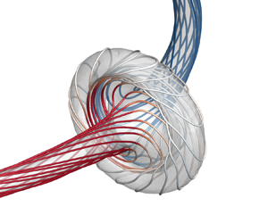
Figure 1. Schematic of closed vortex tubes with complex internal structures in transition and turbulence. (a) Conceptual model of the hairpin vortex in boundary layer transition and a collection of coiled and linked vortex rings in fully developed turbulence, where the flow visualization data were reported in Zheng, Yang & Chen (Reference Zheng, Yang and Chen2016). (b) Closed vortex tube with differential twist on coaxial vortex surfaces and along the vortex centreline. The vortex surfaces are represented by VSF isosurfaces of different isocontour values, with embedded vortex lines (red solid). (c) A segment of the vortex tube in (b), where the vorticity is constructed based on the curved cylindrical coordinates  $(s,\rho,\theta )$, and the vortex centreline $\mathcal {C}$ (blue dash-dotted) is described in the Frenet–Serret frame ( $\boldsymbol {T}$, $\boldsymbol {N}$, $\boldsymbol {B}$).
Coiled vortex lines in a vortex tube can generate twist-wave packets, and their propagation and collision (Melander & Hussain Reference Melander and Hussain1994) can lead to bursting – causing an increase in the local enstrophy and energy dissipation. Vortex bursting has been found in aircraft trailing vortices (Tombach Reference Tombach1973), and addressed in theoretical (Arendt, Fritts & Andreassen Reference Arendt, Fritts and Andreassen1997), experimental (Cuypers, Maurel & Petitjeans Reference Cuypers, Maurel and Petitjeans2003) and numerical studies, but most are restricted to the configuration of vortex columns (Melander & Hussain Reference Melander and Hussain1994; Ji & van Rees Reference Ji and van Rees2022). By contrast, the vortex ring is more common in practical flows (Shariff & Leonard Reference Shariff and Leonard1992) and has a well-defined topological interpretation of helicity in terms of the writhe  $W_r$ and twist $T_w$ (Moffatt & Ricca Reference Moffatt and Ricca1992). Helicity and its decomposition provide a powerful diagnostic tool to understand the complex three-dimensional (3-D) flow dynamics.
Whether helicity conservation can be extended to real dissipative flows is of particular interest and has been extensively studied recently (Kleckner & Irvine Reference Kleckner and Irvine2013; Scheeler et al. Reference Scheeler, van Rees, Kedia, Kleckner and Irvine2017; Kerr Reference Kerr2018a; Meng, Shen & Yang Reference Meng, Shen and Yang2023). For example, Kleckner & Irvine (Reference Kleckner and Irvine2013) experimentally observed that the knotted vortex is quite unstable and transferred to unlinked, coiled vortex rings through viscous reconnection. Numerical studies (Yao, Yang & Hussain Reference Yao, Yang and Hussain2021; Zhao et al. Reference Zhao, Yu, Chapelier and Scalo2021) reveal that the helicity is not conserved during this process: while the initial writhe helicity is destroyed, the local twist rapidly surges at the reconnection site and then travels along the two separated rings. Therefore, studying twist-wave propagation and bursting can shed light not only on the extreme events in turbulence and transition (Moffatt Reference Moffatt2021; Buaria & Pumir Reference Buaria and Pumir2022), but also on the helicity dynamics of flux tubes with complex internal structures.
Studying twist-wave propagation and bursting in a vortex ring, or more generally, in a closed vortex tube, which can be knotted and linked (Ricca, Samuels & Barenghi Reference Ricca, Samuels and Barenghi1999; Kleckner & Irvine Reference Kleckner and Irvine2013; Kerr Reference Kerr2018b; Yao et al. Reference Yao, Yang and Hussain2021), is challenging. First, it is difficult to directly construct a twist wave with a precise amplitude and distribution in a closed vortex tube. Second, in real flows, vortex lines within vortex tubes can have differential twist, i.e. different local twist rates on coaxial vortex surfaces or along the vortex centreline (see figure 1). The differential twist of vortex tubes with finite thickness cannot be characterized by the existing helicity decomposition (Moffatt & Ricca Reference Moffatt and Ricca1992), nor could it be directly measured in previous experiments (Kleckner & Irvine Reference Kleckner and Irvine2013; Scheeler et al. Reference Scheeler, van Rees, Kedia, Kleckner and Irvine2017; Angriman et al. Reference Angriman, Cobelli, Bourgoin, Huisman, Volk and Mininni2021) or numerical simulations (Yao et al. Reference Yao, Yang and Hussain2021; Shen et al. Reference Shen, Yao, Hussain and Yang2022; Yao et al. Reference Yao, Shen, Yang and Hussain2022). The existing ribbon model (Moffatt & Tsinober Reference Moffatt and Tsinober1992; Chui & Moffatt Reference Chui and Moffatt1995) for twisting is restricted to a vortex tube with uniform twist, and it cannot characterize the internal twisting structure of vortex tubes.
We develop a novel helicity decomposition – along with numerical construction and measurement methods – for the differential twist. Moreover, the vortex-surface field (VSF) (Yang & Pullin Reference Yang and Pullin2010, Reference Yang and Pullin2011) is used to track and measure the twist of vortex lines. These methods facilitate the first quantitative study of bursting vortex rings with differential twist.
2. Twisting helicity for differential twist
We introduce here a definition for the differential twist and explain its relation to the helicity. The total helicity
 \begin{equation} H=\int_\mathcal{V} h \,\mathrm{d} \mathcal{V}, \end{equation}
is the volume integral of the helicity density  $h=\boldsymbol u \boldsymbol {\cdot } \boldsymbol \omega$ (Moreau Reference Moreau1961; Moffatt Reference Moffatt1969), with the fluid velocity $\boldsymbol u$ and the vorticity $\boldsymbol \omega =\boldsymbol {\nabla } \times \boldsymbol u$. The helicity of a closed vortex tube can be topologically morphed into $H=\varGamma ^2 (W_r+T_w)$ (Moffatt & Ricca Reference Moffatt and Ricca1992), with $\varGamma$ the total circulation. Note that, while $W_r$ can be obtained from a measurement of the vortex tube centrelines alone, it is difficult to characterize and directly measure $T_w$ in practical flows. As sketched in figure 1(b), the nested coaxial vortex tubes without self-intersection are distinguished by different isosurfaces of a normalized VSF $\phi _v \in [0,1]$. The limiting surface with $\phi _v =1$ represents the vortex centreline $\mathcal {C}$. In figure 1(c), the vortex tube is represented in the curved cylindrical coordinate system $(s,\rho,\theta )$ (Xiong & Yang Reference Xiong and Yang2019, Reference Xiong and Yang2020). Here, $s\in [0,L_C)$ denotes the arclength along $\mathcal {C}$, $L_C$ the length of $\mathcal {C}$, $\rho$ the radial distance from $\mathcal {C}(s)$ and $\theta$ the azimuthal angle from $\boldsymbol N(s)$ in the plane $S_C$ spanned by $\boldsymbol N(s)$ and $\boldsymbol B(s)$, where the unit normal $\boldsymbol N(s)$, binormal $\boldsymbol B(s)$ and tangent $\boldsymbol T(s)$ constitute the Frenet–Serret frame on $\mathcal {C}$. For such vortex tubes with uniform $\boldsymbol \omega$ in $\theta$, $(s,\rho,\theta )$ is simplified to $(s,\phi _v)$.
We derive the contribution of coiled vortex lines on different coaxial vortex surfaces to the total helicity. The twisting helicity (Moffatt & Ricca Reference Moffatt and Ricca1992) of an isolated closed vortex tube can be expressed as
 \begin{equation} H_{T}=\varGamma^2 T_w, \end{equation}
where  $\varGamma$ denotes the circulation and $T_w$ the total twist number of the vortex tube. For closed vortex tubes with uniform twist along $\phi _v$, the twisting number (Fuller Reference Fuller1971; Chui & Moffatt Reference Chui and Moffatt1995)
 \begin{equation} T_{w}=\frac{1}{2 {\rm \pi}} \oint_{\mathcal{C}}(\boldsymbol{N}_s \times \boldsymbol{N}_s^{\prime}) \boldsymbol{\cdot} \boldsymbol{T} \,\mathrm{d} s, \end{equation}
is defined by a ribbon model. Here, the ribbon edges are the vortex centreline  $\mathcal {C}$ and a vortex line $\mathcal {C}^{*}$. Moreover, $\boldsymbol {N}_s$ denotes a radial unit vector from $\mathcal {C}$ pointing to $\mathcal {C}^{*}$ in plane $S_C$ (see figure 1c), and $\boldsymbol {N}_s^{\prime }=\mathrm {d} \boldsymbol {N}_s / \mathrm {d} s$; $\boldsymbol {T}$ is the unit tangent vector of $\mathcal {C}$. This definition requires that every vortex line has the same value of $T_w$ calculated from (2.3), so it is restricted to characterizing a vortex tube with uniform twist or a differential twist along the vortex centreline.
In order to characterize the differential twist both along the vortex centreline and on different vortex surfaces, we establish a more complete definition of  $T_w$ than (2.3). For generalized closed tubes with differential twist, we introduce the local twist rate
 \begin{equation} \eta\left(s,\phi_{v}\right)=\left(\boldsymbol{N}_{s} \times \boldsymbol{N}_{s}^{\prime}\right) \boldsymbol{\cdot} \boldsymbol{T}, \end{equation}
for a vortex line on a vortex surface of  $\phi _v$ at different locations, and the circulation
 \begin{equation} \varGamma_\phi=\varGamma_\phi(\phi_v) \in [0,\varGamma], \end{equation}
through the tube enclosed by a vortex surface of  $\phi _v$. If $\eta$ is circumferentially uniform on each vortex surface, i.e. $\eta$ is constant on the intersection of the isosurface of $\phi _v$ and the plane $S_C$ normal to $\mathcal {C}$, we define the twisting number
 \begin{equation} T_{\phi}\left(\phi_{v}\right)=\frac{1}{2{\rm \pi}}\oint_{\mathcal{C}} \eta\left(s,\phi_{v}\right)\,\mathrm{d} s, \end{equation}
for each vortex surface.
We first calculate the twisting helicity  $\Delta H_{T}(\varPhi )$ for a single vortex surface of $\phi _v=\varPhi$ (see figure 2) with a given constant $\varPhi$. This surface with infinitesimal thickness has $\varGamma _{\phi }(\varPhi )$ and $T_\phi (\varPhi )$. As illustrated in figure 2
 \begin{equation} \Delta H_{T}(\varPhi) = \bar{H}_{T,1} - \bar{H}_{T,2}, \end{equation}
of a twisted vortex tube can be obtained by the difference of twisting helicities for two adjacent co-axial virtual vortex tubes 1 and 2 with
 \begin{equation} \bar{\varGamma}_1 = \varGamma_{\phi}\left(\varPhi\right), \quad \bar{T}_{w,1} =T_{\phi}\left(\varPhi\right), \end{equation}
and
 \begin{equation} \bar{\varGamma}_2 = \varGamma_{\phi}\left(\varPhi+\Delta\phi_v\right), \quad \bar{T}_{w,2} =T_{\phi}\left(\varPhi\right), \end{equation}
respectively, where the overline denotes the quantity in a virtual tube. All co-axial vortex surfaces inside the two virtual tubes have the same twist distribution as the vortex surface  $\phi _v=\varPhi$, so the two virtual tubes have uniform twist along $\phi _v$ and their twisting helicities can be obtained by (2.2).

Figure 2. Schematic for calculating the twisting helicity of a vortex surface with infinitesimal thickness by two adjacent co-axial virtual tubes with uniform twist along  $\phi _v$. The vortex surface of $\phi _v=\varPhi$ is peeled off from the vortex tube with differential twist along $s$ and $\phi _v$. All co-axial vortex surfaces inside the two virtual tubes have the same twist distribution as the vortex surface of $\phi _v=\varPhi$.
Substituting (2.2), (2.8a,b) and (2.9a,b) into (2.7) yields
 \begin{equation} \Delta H_{T}(\varPhi) = \varGamma_\phi(\varPhi)^2 T_\phi(\varPhi) - \varGamma_\phi(\varPhi+\Delta\phi_v)^2 T_\phi(\varPhi). \end{equation}
Applying the Taylor expansion of  $\varGamma _\phi (\varPhi +\Delta \phi _v)$ to (2.10) yields
 \begin{equation} \Delta H_{T}(\varPhi) ={-}2\varGamma_\phi(\varPhi)\frac{\mathrm{d}\varGamma_\phi(\varPhi)}{\mathrm{d}\phi_v}T_\phi(\varPhi)\Delta\phi_v+O(\Delta\phi_v^2). \end{equation}
Then, we obtain
 \begin{equation} \frac{\mathrm{d} H_{T}(\varPhi)}{\mathrm{d} \phi_v}=\lim_{\Delta \phi_v\rightarrow 0} \frac{\Delta H_{T}(\varPhi)}{\Delta \phi_v}={-}2\varGamma_\phi(\varPhi)\frac{\mathrm{d}\varGamma_\phi(\varPhi)}{\mathrm{d}\phi_v}T_\phi(\varPhi). \end{equation}
Thus each vortex surface of  $\phi _v$ in a vortex tube with differential twist along $s$ and $\phi _v$ has
 \begin{equation} \mathrm{d} H_{T}(\phi_v)={-}2\varGamma_\phi(\phi_v)\frac{\mathrm{d}\varGamma_\phi(\phi_v)}{\mathrm{d}\phi_v}T_\phi(\phi_v) \,\mathrm{d} \phi_v. \end{equation}
Finally, we obtain the total twisting helicity
 \begin{equation} H_{T}={-}\frac{1}{\rm \pi}\int_{0}^{1}\varGamma_\phi(\phi_v)\frac{\mathrm{d}\varGamma_\phi(\phi_v)}{\mathrm{d}\phi_v} \left( \oint_{\mathcal{C}} \eta(s,\phi_v) \,\mathrm{d} s \right) \,\mathrm{d}\phi_v, \end{equation}
of a vortex tube with the total circulation  $\varGamma$ and differential twist along $s$ and $\phi _v$ by the integration $\int \,\mathrm {d} H_T$ with (2.6), which is a circulation-weighted average of twisting numbers over all co-axial vortex surfaces. Substituting (2.14) into (2.2) yields
 \begin{equation} T_w={-}\frac{1}{{\rm \pi}\varGamma^2}\int_{0}^{1}\varGamma_\phi(\phi_v)\frac{\mathrm{d}\varGamma_\phi(\phi_v)}{\mathrm{d}\phi_v} \left( \oint_{\mathcal{C}} \eta(s,\phi_v) \,\mathrm{d} s \right) \,\mathrm{d}\phi_v. \end{equation}
This equation is further verified with several numerical examples in Appendix A.
3. Construction of differential twist
We construct the vorticity field  $\boldsymbol {\omega }$ for a closed vortex tube with differential twist. This construction method with its numerical algorithm is an extension of that in Xiong & Yang (Reference Xiong and Yang2019, Reference Xiong and Yang2020) by incorporating variations of the core size and local twist rate in terms of $s$ and $\phi _v$.
First, the tube centreline  $\mathcal {C}$ is described by a given parametric equation
 \begin{equation} \boldsymbol{x}=\boldsymbol{c}(s)+\rho \cos \theta \boldsymbol{N}(s)+\rho \sin \theta \boldsymbol{B}(s). \end{equation}
The Frenet–Serret formulas on  $\mathcal {C}$ are
 \begin{equation} \left. \begin{aligned} \frac{\mathrm{d} \boldsymbol{T}}{\mathrm{d} s} & =\kappa \boldsymbol{N}, \\ \frac{\mathrm{d} \boldsymbol{N}}{\mathrm{d} s} & ={-}\kappa \boldsymbol{T}+\tau \boldsymbol{B}, \\ \frac{\mathrm{d} \boldsymbol{B}}{\mathrm{d} s} & ={-}\tau \boldsymbol{N}, \end{aligned} \right\} \end{equation}
where  $\kappa$ is the curvature and $\tau$ is the torsion of $\mathcal {C}$.
Based on coordinates ( $s, \rho, \theta$), we specify
 \begin{equation} \boldsymbol{\omega}(s, \rho, \theta)= \omega_s(s,\rho)\boldsymbol{e}_{s}+\omega_\rho(s,\rho,\theta)\boldsymbol{e}_{\rho}+\omega_\theta(s,\rho,\theta)\boldsymbol{e}_{\theta}, \end{equation}
of a vortex tube, where the local frame is spanned by unit vectors
 \begin{equation} \left. \begin{aligned} \boldsymbol{e}_{s} & =\boldsymbol{T}, \\ \boldsymbol{e}_{\rho} & =\cos \theta \boldsymbol{N}+\sin \theta \boldsymbol{B}, \\ \boldsymbol{e}_{\theta} & ={-}\sin \theta \boldsymbol{N}+\cos \theta \boldsymbol{B}. \end{aligned} \right\} \end{equation}
By setting the variable initial core size  $\sigma (s)$ and local twist rate $\eta (s,\phi _v)$, vorticity components $\omega _s(s,\rho )$ and $\omega _\theta (s,\rho,\theta )$ are determined by introducing $\sigma (s)$ and $\eta (s,\phi _v)$ into the construction method in Xiong & Yang (Reference Xiong and Yang2020) and Shen et al. (Reference Shen, Yao, Hussain and Yang2022) and then $\omega _\rho (s,\rho,\theta )$ is solved from the divergence-free constraint. Thus the vorticity of closed vortex tubes with differential twist and variable thickness is specified as
 \begin{equation} \boldsymbol{\omega}(s,
\rho, \theta)=\varGamma
f(s,\rho)\left[\underbrace{\boldsymbol{e}_{s}}_{\textit{flux}}+\underbrace{\frac{\mathrm{d}
\sigma(s)}{\mathrm{d}
s}\frac{\rho\boldsymbol{e}_{\rho}}{\sigma(s)(1-\kappa(s)
\rho \cos \theta)}}_{\textit{tube
thickness}}+\underbrace{\frac{\rho \eta(s, \phi_v)
\boldsymbol{e}_{\theta}}{1-\kappa(s) \rho \cos
\theta}}_{\textit{twist}} \right],
\end{equation}
\begin{equation} \boldsymbol{\omega}(s,
\rho, \theta)=\varGamma
f(s,\rho)\left[\underbrace{\boldsymbol{e}_{s}}_{\textit{flux}}+\underbrace{\frac{\mathrm{d}
\sigma(s)}{\mathrm{d}
s}\frac{\rho\boldsymbol{e}_{\rho}}{\sigma(s)(1-\kappa(s)
\rho \cos \theta)}}_{\textit{tube
thickness}}+\underbrace{\frac{\rho \eta(s, \phi_v)
\boldsymbol{e}_{\theta}}{1-\kappa(s) \rho \cos
\theta}}_{\textit{twist}} \right],
\end{equation}
with the Gaussian kernel function
 \begin{equation} f(s,\rho)=\left\{
\begin{array}{@{}lll} \dfrac{1}{2{\rm \pi}\sigma(s)^2}\exp\left[
\dfrac{-\rho^2}{2\sigma(s)^2}\right] , & s \in [0,L_C), &
\rho \in [0,R_v),\\ 0, & s \in [0,L_C), & \rho \in
[R_v,+\infty), \end{array} \right.
\end{equation}
\begin{equation} f(s,\rho)=\left\{
\begin{array}{@{}lll} \dfrac{1}{2{\rm \pi}\sigma(s)^2}\exp\left[
\dfrac{-\rho^2}{2\sigma(s)^2}\right] , & s \in [0,L_C), &
\rho \in [0,R_v),\\ 0, & s \in [0,L_C), & \rho \in
[R_v,+\infty), \end{array} \right.
\end{equation}
and the initial normalized VSF
 \begin{equation} \phi_{v}(s,\rho)= 2{\rm \pi}\sigma(s)^2f(s,\rho) \in [0,1], \end{equation}
where the three terms on the right-hand side of (3.5) represent the vorticity flux, tube thickness and twist terms of  $\boldsymbol \omega$, respectively.
If  $\kappa (s) = 0$ and $\eta (s,\phi _v) = 0$, (3.5) degenerates into the vorticity for a straight vortex tube with a variable core size (Ji & van Rees Reference Ji and van Rees2022). If $\sigma (s)$ and $\eta (s,\phi _v)$ are constants, (3.5) degenerates into a constant-thickness vortex tube with uniform twist (Xiong & Yang Reference Xiong and Yang2020; Shen et al. Reference Shen, Yao, Hussain and Yang2022).
As proved below, the vector field constructed by (3.5) is solenoidal, which can be used as a vorticity or magnetic field.
Theorem 1 The vector field  $\boldsymbol {\omega }$ constructed by (3.5) is divergence free.
Proof. In the curved cylindrical coordinate system, by applying the inverse function theorem to the Jacobian matrix (Xiong & Yang Reference Xiong and Yang2020) between  $(s, \rho, \theta )$ and $(x,y,z)$, we derive
 \begin{equation} \left. \begin{aligned} & \boldsymbol{\nabla} s=\frac{\boldsymbol{T}}{1-\kappa \rho \cos \theta}, \\ & \boldsymbol{\nabla} \rho=\cos \theta \boldsymbol{N}+\sin \theta \boldsymbol{B}, \\ & \boldsymbol{\nabla} \theta=\frac{-\tau}{1-\kappa \rho \cos \theta} \boldsymbol{T}+\frac{1}{\rho}\left(-\sin \theta \boldsymbol{N}+\cos \theta \boldsymbol{B}\right). \end{aligned} \right\} \end{equation}
Taking the divergence of (3.3) yields
 \begin{equation} \boldsymbol{\nabla} \boldsymbol{\cdot} \boldsymbol{\omega}= \boldsymbol{\nabla}\boldsymbol{\cdot} \left(\omega_s\boldsymbol{e}_{s}\right)+\boldsymbol{\nabla}\boldsymbol{\cdot} (\omega_\rho\boldsymbol{e}_{\rho})+\boldsymbol{\nabla}\boldsymbol{\cdot} \left(\omega_\theta\boldsymbol{e}_{\theta}\right), \end{equation}
and using (3.4) yields
 \begin{align}
\boldsymbol{\nabla}\boldsymbol{\cdot}
(\omega_s\boldsymbol{e}_{s}) &=\left(\frac{\partial
\omega_s}{\partial s}\boldsymbol{\nabla} s +\frac{\partial
\omega_s}{\partial \rho}\boldsymbol{\nabla} \rho\right)
\boldsymbol{T}+ \omega_s \frac{\text{d}
\boldsymbol{T}}{\text{d}
s}\boldsymbol{\cdot}\boldsymbol{\nabla} s,\end{align}
\begin{align}
\boldsymbol{\nabla}\boldsymbol{\cdot}
(\omega_s\boldsymbol{e}_{s}) &=\left(\frac{\partial
\omega_s}{\partial s}\boldsymbol{\nabla} s +\frac{\partial
\omega_s}{\partial \rho}\boldsymbol{\nabla} \rho\right)
\boldsymbol{T}+ \omega_s \frac{\text{d}
\boldsymbol{T}}{\text{d}
s}\boldsymbol{\cdot}\boldsymbol{\nabla} s,\end{align}
 \begin{align}\boldsymbol{\nabla}\boldsymbol{\cdot}
(\omega_\rho\boldsymbol{e}_{\rho}) &=\left(\frac{\partial
\omega_\rho}{\partial s}\boldsymbol{\nabla} s
+\frac{\partial \omega_\rho}{\partial
\rho}\boldsymbol{\nabla} \rho+\frac{\partial
\omega_\rho}{\partial \theta}\boldsymbol{\nabla}
\theta\right) (\cos \theta \boldsymbol{N}+\sin \theta
\boldsymbol{B})\nonumber\\ &\quad+ \omega_\rho
\left(-\sin\theta\boldsymbol{\nabla}\theta\boldsymbol{\cdot}\boldsymbol{N}+\cos\theta\frac{\text{d}
\boldsymbol{N}}{\text{d}
s}\boldsymbol{\cdot}\boldsymbol{\nabla} s
+\cos\theta\boldsymbol{\nabla}\theta\boldsymbol{\cdot}\boldsymbol{B}+\sin\theta\frac{\text{d}
\boldsymbol{B}}{\text{d}
s}\boldsymbol{\cdot}\boldsymbol{\nabla}
s\right), \end{align}
\begin{align}\boldsymbol{\nabla}\boldsymbol{\cdot}
(\omega_\rho\boldsymbol{e}_{\rho}) &=\left(\frac{\partial
\omega_\rho}{\partial s}\boldsymbol{\nabla} s
+\frac{\partial \omega_\rho}{\partial
\rho}\boldsymbol{\nabla} \rho+\frac{\partial
\omega_\rho}{\partial \theta}\boldsymbol{\nabla}
\theta\right) (\cos \theta \boldsymbol{N}+\sin \theta
\boldsymbol{B})\nonumber\\ &\quad+ \omega_\rho
\left(-\sin\theta\boldsymbol{\nabla}\theta\boldsymbol{\cdot}\boldsymbol{N}+\cos\theta\frac{\text{d}
\boldsymbol{N}}{\text{d}
s}\boldsymbol{\cdot}\boldsymbol{\nabla} s
+\cos\theta\boldsymbol{\nabla}\theta\boldsymbol{\cdot}\boldsymbol{B}+\sin\theta\frac{\text{d}
\boldsymbol{B}}{\text{d}
s}\boldsymbol{\cdot}\boldsymbol{\nabla}
s\right), \end{align}
 \begin{align} \boldsymbol{\nabla}\boldsymbol{\cdot} (\omega_\theta\boldsymbol{e}_{\theta}) &=\left(\frac{\partial \omega_\theta}{\partial s}\boldsymbol{\nabla} s +\frac{\partial \omega_\theta}{\partial \rho}\boldsymbol{\nabla} \rho+\frac{\partial \omega_\theta}{\partial \theta}\boldsymbol{\nabla} \theta\right) (-\sin \theta \boldsymbol{N}+\cos \theta \boldsymbol{B})\nonumber\\&\quad+ \omega_\theta \left(-\cos\theta\boldsymbol{\nabla}\theta\boldsymbol{\cdot}\boldsymbol{N}-\sin\theta\frac{\text{d} \boldsymbol{N}}{\text{d} s}\boldsymbol{\cdot}\boldsymbol{\nabla} s -\sin\theta\boldsymbol{\nabla}\theta\boldsymbol{\cdot}\boldsymbol{B}+\cos\theta\frac{\text{d} \boldsymbol{B}}{\text{d} s}\boldsymbol{\cdot}\boldsymbol{\nabla} s\right). \end{align}
Substituting (3.2) and (3.4) into (3.10), (3.11) and (3.12), and considering the orthogonality of the Frenet–Serret frame yields
 \begin{equation} \left. \begin{aligned} & \boldsymbol{\nabla}\boldsymbol{\cdot} (\omega_s\boldsymbol{e}_{s}) =\frac{1}{1-\kappa\rho\cos\theta}\frac{\partial \omega_s}{\partial s},\\ & \boldsymbol{\nabla}\boldsymbol{\cdot} (\omega_\rho\boldsymbol{e}_{\rho}) =\frac{\partial \omega_\rho}{\partial \rho}+\frac{1-2\kappa\rho\cos\theta}{\rho(1-\kappa\rho\cos\theta)}\omega_\rho,\\ & \boldsymbol{\nabla}\boldsymbol{\cdot} (\omega_\theta\boldsymbol{e}_{\theta}) =\frac{1}{\rho}\frac{\partial \omega_\theta}{\partial \theta}+\frac{\kappa\sin\theta}{1-\kappa\rho\cos\theta}\omega_\theta. \end{aligned} \right\} \end{equation}
 For  $\rho \geqslant R_v$, we have $\boldsymbol {\omega }=0$ from (3.6). For $\rho < R_v$, substituting (3.5) and (3.6) into (3.13) yields
 \begin{equation} \left. \begin{aligned} & \boldsymbol{\nabla}\boldsymbol{\cdot} (\omega_s\boldsymbol{e}_{s}) =\frac{\varGamma(\rho^2-2\sigma^2)}{2{\rm \pi}\sigma^5(1-\kappa\rho\cos\theta)}\frac{\mathrm{d} \sigma}{\mathrm{d} s}\exp\left( \frac{-\rho^2}{2\sigma^2}\right),\\ & \boldsymbol{\nabla}\boldsymbol{\cdot} (\omega_\rho\boldsymbol{e}_{\rho}) =\frac{\varGamma(2\sigma^2-\rho^2)}{2{\rm \pi}\sigma^5(1-\kappa\rho\cos\theta)}\frac{\mathrm{d} \sigma}{\mathrm{d} s}\exp\left( \frac{-\rho^2}{2\sigma^2}\right),\\ & \boldsymbol{\nabla}\boldsymbol{\cdot} (\omega_\theta\boldsymbol{e}_{\theta}) =0, \end{aligned} \right\} \end{equation}
after some algebra. Finally we obtain  $\boldsymbol {\nabla } \boldsymbol {\cdot } \boldsymbol {\omega }=0$.
The numerical implementation is detailed in Appendix A. Typical examples constructed by (3.5) in figure 3 show coiled vortex lines with differential twist lying on various closed vortex tubes. Furthermore, we develop a numerical method to measure the local twisting rate on a vortex surface for given  $\boldsymbol \omega$ and $\phi$. The algorithm is based on multiple vortex lines in terms of the discrete arclength on the VSF isosurface, which is detailed in Appendix B. Thus, we can quantify the evolution of coiling vortex lines on different vortex surfaces in a viscous evolution.

Figure 3. Closed vortex tubes with various internal structures. These closed vortex tubes with arbitrary topology, differential twist and variable thickness are constructed by (3.5): (a) trivial ring, (b) trefoil knot and (c) figure-eight knot. They are visualized by VSF isosurfaces with embedded vortex lines. The inner and outer tubes in (a) are two VSF isosurfaces with different colours; the surfaces in (b,c) are colour coded by  $h$.
$h$.
4. Results
4.1. Evolution of vortex ring with differential twist
We highlight the role of differential twist in helicity and vortex dynamics via direct numerical simulation (DNS) of bursting of vortex rings. Initial twisted vortex rings with a radius  $R_0=1$ are constructed by (3.5), with initial $\varGamma =\varGamma _0=1$ and $\sigma =\sigma _0=1/(8\sqrt {2{\rm \pi} })$. The initial local twist rate $\eta (s,\phi _{v})=\eta _0=A \sin (s/R_0)$ varies along $\mathcal {C}$. We use the constructed vorticity fields in (3.5) as initial conditions, and calculate their evolutions using DNS. The 3-D incompressible Navier–Stokes equations are solved in the vorticity–velocity form (Wu, Ma & Zhou Reference Wu, Ma and Zhou2015) using the pseudo-spectral method in a periodic box of size $L=2 {\rm \pi}$ on $N^{3}$ uniform grid points. The numerical solver removes aliasing errors using the two-third truncation method with the maximum wavenumber $k_{max} \approx N / 3$. The time integration is treated by the explicit second-order Runge–Kutta scheme in physical space, with the adaptive time step ensuring the small enough Courant–Friedrichs–Lewy number for numerical stability and accuracy. The vortex Reynolds number is set to ${\textit {Re}}\equiv \varGamma /\nu =2000$. To ensure that the grid resolution can fully resolve the flow evolution, $N$ is carefully chosen to be $512$, $768$ and $1024$ for the initial twist amplitudes $A=10$, 20 and 30, respectively. For each case, we carried out the grid convergence test and confirmed that the DNS results converge for $N$ to ensure that the grid resolution fully resolves the flow evolution.
In addition, the VSF evolution is calculated using the two-time method (Yang & Pullin Reference Yang and Pullin2011) and its implementation is reported in Appendix C. The Lagrangian-like evolution of the twisted vortex ring with  $A=20$ and $Re=2000$ is visualized by the isosurface of $\phi _v=0.5$ in figure 4. At $t=0$, two twist waves of vortex lines with opposite chiralities travel in opposite directions. Each wave packet is similar to a Kelvin wave with zero azimuthal wavenumber (Arendt et al. Reference Arendt, Fritts and Andreassen1997; Fabre, Sipp & Jacquin Reference Fabre, Sipp and Jacquin2006). Then, they collide and burst at the upper symmetric plane $SP_1$, forming a disk-like vortex dipole structure. Meanwhile, the axial gradient of the core size near the bursting site regenerates secondary twist waves, which propagate backward and cause secondary bursting at the lower symmetric plane $SP_2$ after $t = 2$. Note that, as shown in Ji & van Rees (Reference Ji and van Rees2022) for a vortex column, such successive bursting can also be triggered by a vortex ring with initial core-size perturbation (see Appendix D).

Figure 4. Lagrangian-like evolution of vortex surfaces and lines. The visualization shows the evolution of the VSF isosurface (colour coded by  $h$) of $\phi _v = 0.5$ for $A=20$ and $Re=2000$. Some attached vortex lines are integrated from points on the isosurface. Note that $t=t/(R_0^2/\varGamma _0)$ is non-dimensionalized here. The close-up view shows vortex lines (colour coded by $h$) on the VSF isosurface (translucent) of $\phi _v=0.7$ at $t=0.75$ in vortex bursting.
In figure 5(a), the enstrophy  $\varOmega (t) = \int _\mathcal {V} |\boldsymbol {\omega }|^{2}/2 \,\mathrm {d} \mathcal {V}$ in the viscous evolution decays and shows a bump during bursting. For comparison, viscous diffusion of a vortex column shows exponential decay of $\varOmega$. Due to the initial symmetry, $H$ remains zero, and the positive and negative parts $H^\pm =\int _{\mathcal {V}} h^{\pm } \,\mathrm {d} \mathcal {V}$ of $H$ characterize the amplitudes of the counter-rotating waves. Before bursting, the core dynamics induced meridional flow (Melander & Hussain Reference Melander and Hussain1994) uncoils vortex lines and thickens the local vortex tube to form an axial core-size gradient. The vortex tube with the axial core-size variation then re-coils the vortex lines. Thus, $|H^\pm |$ first decays and then rebounds in figure 5(b). The viscous decay of $H^\pm$ (solid line) is faster than that of the uniform helicity model (dash-dotted line), because $\eta$, which is proportional to the viscous decay rate of twist (Yao et al. Reference Yao, Yang and Hussain2021; Shen et al. Reference Shen, Yao, Hussain and Yang2022), is more locally concentrated and larger than in the latter.

Figure 5. Flow statistics. (a,b) Evolution of (a)  $\varOmega$ and (b) $H$ (black), $H^+$ (red) and $H^-$ (blue) for various $A$. The dash-dotted lines denote modelling results $\varOmega (t)=\varOmega _{0} \exp [-\int _{0}^{t}2 \nu (\sigma _0^{2}+2\nu t)^{-1} \,\mathrm {d} t]$ and $H(t)=H_0 \exp [-\int _{0}^{t}2 \nu (\sigma _0^{2}+2\nu t)^{-1} \,\mathrm {d} t]$ for a uniformly twisted vortex column with $A=20$. The peak heights of $\varOmega$ and $|H^\pm |$ grow with $A$, while the height of the secondary peak of $|H^\pm |$ is the highest for $A=20$. (c–e) Local twist rates on different VSF isosurfaces along the vortex centreline at (c) $t=0.25$, (d) 0.5 and (e) 1.5 for $A=20$. Arrows in (c,e) denote the propagating direction of twist-wave packets. The inset in (d) shows entire profiles of $\eta$.
4.2. Vortex bursting
During the evolution, the twist propagates along  $\mathcal {C}$ and varies with $\phi _v$. Figure 5(c) plots the distribution of $\eta$ along $s$ on different vortex surfaces at $t=0.25$ for $A=20$ and $Re=2000$. At early times, two peaks of $\eta$ approach each other and evolve towards a discontinuity, similar to shock formation. The propagation speed of twist waves grows with $\phi _v$; i.e. the waves travel faster on an inner vortex surface than on an outer surface.
We develop an inviscid model for the propagation of twist vortex waves, which can predict when the vortex bursting occurs. The twist waves are modelled as travelling waves along the vortex centreline, so that their propagation speed equals the axial velocity of the local fluid. Thus, we have
 \begin{equation} \eta(s,\phi_v,t)=F(s-u_s t,\phi_v), \end{equation}
with a function  $F$. The axial velocity (Yao et al. Reference Yao, Yang and Hussain2021) of a uniformly twisted vortex tube with constant $\eta$ is obtained by the Biot–Savart law as
 \begin{equation} u_s(\rho)=\frac{\varGamma \eta}{2 {\rm \pi}} \exp \left(\frac{-\rho^{2}}{2 \sigma^{2}}\right). \end{equation}
Substituting the initial VSF profile  $\phi _{v}(\rho )$ into (4.2) and replacing the constant $\eta$ by a varying one yield the axial velocity
 \begin{equation} u_s(s,\phi_v)=\frac{\varGamma\phi_v\eta(s,\phi_v,t)}{2{\rm \pi}}, \end{equation}
of a vortex surface with differential twist. Based on (4.1) and (4.3), we obtain a Burgers-like equation
 \begin{equation} \left.
\begin{array}{ll@{}} \dfrac{\partial \eta}{\partial
t}+\dfrac{\varGamma \phi_{v} \eta}{2 {\rm \pi}} \dfrac{\partial
\eta}{\partial s}=0, & s \in[0,L_C),\quad t>0,\\
\eta\left(s,\phi_{v},
0\right)=\eta_{0}\left(s,\phi_{v}\right), & \end{array}
\right\} \end{equation}
\begin{equation} \left.
\begin{array}{ll@{}} \dfrac{\partial \eta}{\partial
t}+\dfrac{\varGamma \phi_{v} \eta}{2 {\rm \pi}} \dfrac{\partial
\eta}{\partial s}=0, & s \in[0,L_C),\quad t>0,\\
\eta\left(s,\phi_{v},
0\right)=\eta_{0}\left(s,\phi_{v}\right), & \end{array}
\right\} \end{equation}
where  $L_C$ denotes the length of $\mathcal {C}$ and $\eta _{0}(s,\phi _{v})$ the given initial $\eta$. Note that this model is an inviscid approximation, and the twist wave can have dispersion in viscous flows.
From the solution to (4.4)
 \begin{equation} \eta(s,\phi_v,t)=\eta_0\left(s-\frac{\varGamma\phi_v\eta}{2{\rm \pi}}t,\phi_v\right) ,\quad t< t_b, \end{equation}
we obtain that  $\partial \eta _{0}/\partial s$ becomes infinite at the blow-up time
 \begin{equation} t_{b}(\phi_v)=\min \left.\left[\left(-\frac{\varGamma \phi_{v}}{2 {\rm \pi}} \frac{\partial \eta_{0}}{\partial s}\right)^{{-}1}\right]\right|_{{\partial \eta_{0}}/{\partial s}<0}. \end{equation}
With  $\eta _0(s,\phi _{v})=A \sin (s/R_0)$, (4.6) gives an estimation of the vortex bursting time $t_b(\phi _v) = 2{\rm \pi} R_0/(\varGamma _0A\phi _v)$ for an isosurface of $\phi _v$. It decreases with $\phi _v$, so the bursting develops gradually from the vortex centreline to its outer surfaces, and the earliest blow-up time is $t_{b}(\phi _v=1)={\rm \pi} /10 \approx 0.314$ for $A=20$. The comparison of the DNS and modelling results for the evolution of $\eta$ (see figure 6) shows that (4.5) provides a satisfactory estimate of the local twist rate.

Figure 6. Comparison of DNS (symbols) and modelling (solid lines) results of  $\eta$ on VSF isosurfaces of $\phi _v =0.1$ (red), $0.5$ (green) and $0.9$ (blue) at $t=0.25$. The model predictions calculated from (4.5) capture different propagation speeds on different vortex surfaces, in close agreement with the DNS results.
In figure 5(d), the coiling of vortex lines gradually accumulates on both sides of  $SP_1$ at $s/L_C=0.5$ after $t = {\rm \pi}/10$. The surge of $\eta$ characterizes incipient vortex bursting. Consistent with the model of $t_b$, bursting first occurs near the vortex centreline (with large $\phi _v$). In particular, the spikes of $\eta (s,\phi _v=0.9)$ have a maximum value around 160 at $t=0.5$ (see the inset) and are more than 10 times the averaged initial amplitude $2A/{\rm \pi}$. As illustrated in the close-up view in figure 4, vortex surfaces are flattened on $SP_1$ and rolled up at their edge, forming a disk-like structure with highly spiral vortex lines. The local flow topology at the bursting site is similar to the statistically preferential state of the bi-axial strain in turbulence (Meneveau Reference Meneveau2011).
The formation and decay of the disk structure significantly alter the radial tube size near  $SP_1$, triggering the generation of secondary counter-twist waves (Ji & van Rees Reference Ji and van Rees2022). In figure 5(e), new twist waves are first generated at large $\phi _v$ near $\mathcal {C}$. Subsequently, the chirality of twist waves on outer vortex surfaces is reversed from inner to outer layers. The secondary twist waves gradually intensify and cause the secondary bursting on $SP_2$.
4.3. Effect of initial twist amplitude
During bursting, larger  $A$ (or higher $Re$) can cause a more complex vortex dynamics. Increasing $A$ from 20 to 30 in figure 7(a), the VSF visualization reveals that vortex reconnection occurs within larger disk structures. As sketched in figure 7(b), the spiral vortex lines are pressed onto the disk, and the reconnection of each line at two locations (marked by dashed circles) pinches off a vortex loop from the rolling-up edge of the disk. Strongly coiled vortex lines are uncoiled immediately after reconnection, causing a drop in local core size and twist rate of the main tube. The major secondary ring structure with vanishing flux consists of the pinched-off vortex loops. It is also called the vortex dipole tube (Hussain & Stout Reference Hussain and Stout2013) whose cross-section is a pair of concentrated vorticity regions with opposite signs. The successive reconnection of vortex lines is asymmetric in the $\theta$-direction due to the curved vortex centreline, which is distinctly different from the symmetric reconnection in bursting of a rectilinear vortex tube (Ji & van Rees Reference Ji and van Rees2022).

Figure 7. Vortex reconnection for the bursting vortex ring. (a) Evolution of the VSF isosurface  $\phi _v = 0.3$ for $A=30$ with some attached vortex lines (colour coded by $h$) before and after reconnection (from $t=0.9$ to $t=1.4$). (b) Schematic of the vortex reconnection that occurs in the bursting disk. Red and blue lines represent right- and left-handed coiled vortex lines, respectively. Dashed circles mark reconnection locations of a vortex line. Translucent green sections illustrate the sudden loss of the vortex tube thickness after the reconnection, where the dipole tube formed after the reconnection consists of vortex dipoles.
In figure 5(b), the second peak of  $|H^\pm |$ of $A=20$ around $t=3$ after bursting is the highest, even slightly higher than $A=30$, implying that secondary twist waves are weakened by vortex reconnection. The amplitude of the secondary twist wave is positively correlated with the axial gradient of the vortex core size (Ji & van Rees Reference Ji and van Rees2022). Although stronger twist-wave collision can produce a larger disk, the reconnection significantly reduces the core size (and its axial gradient) of the disk (see figure 7b). After reconnection, the reduction of the core-size gradient inhibits the regeneration of strong twist waves and pre-empts subsequent bursting.
The cancellation and regeneration of right- or left-handed twist waves on different vortex surfaces can be quantified based on  $T_\phi ^+$ or $T_\phi ^-$, defined as $T_\phi ^\pm (\phi _v)=\oint _{\mathcal {C}} \eta ^\pm \,\mathrm {d} s$ with
 \begin{equation} \eta^{+}= \begin{cases}\eta, & \text{if } \eta \geqslant 0, \\ 0, & \text{otherwise},\end{cases} \end{equation}
and  $\eta ^-=\eta -\eta ^+$. The evolution of $T_\phi ^+$ is shown in figure 8. After the first bursting, secondary twist waves regenerate successively from inner to outer vortex surfaces. The regeneration of $T_\phi ^+$ for $A=30$ with slope 2/3 is weaker than for $A=20$ with slope 4/3, confirming weakened secondary twist waves.

Figure 8. Effect of the vortex reconnection on the strength of twist waves. Evolution of  $T_\phi ^+$ on different VSF isosurfaces for $A=20$ ((a), without reconnection) and $A=30$ ((b), with reconnection) at $Re=2000$, along with guide lines (dotted) after the vortex bursting with slopes of $4/3$ and $2/3$, respectively.
5. Discussion
We develop a helicity decomposition that allows computation of the differential twist within vortex tubes. The decomposition is used to study the propagation of twist waves within a vortex ring and the bursting due to their collision. In particular, we establish a theoretical relation (2.15) between  $H$ and $\eta$ of vortex lines on different coaxial vortex surfaces, along with the numerical measurement of $\eta$ based on VSF; DNS cases of bursting vortex rings are set up with differential twists. Two twist waves with opposite helical chiralities collide on the ring cross-section, where the local twist rate surges by over 10 times the average initial amplitude. The propagation speed is faster on inner vortex surfaces than on outer ones. The dynamics of vortex bursting and the bursting time are modelled by a Burgers-like equation. During the bursting, local vortex surfaces are squeezed to form a disk-like dipole structure with strongly coiled vortex lines. With larger initial twisting rates, vortex reconnection pinches dipole vortex rings off from the rolling-up edge of the bursting disk and significantly reduces the core-size gradient to inhibit subsequent bursting.
The rapid coiling and stretching of vortex lines can destabilize their vortical structures and trigger transition. As a heuristic model problem, the propagation of twist waves and bursting of a vortex ring can be further used to study extreme events of the vorticity/helicity dynamics in transition and turbulence and to explore the possible formation of finite-time singularities in the Euler dynamics. Moreover, the construction and diagnostic methods of the differential twist provide a complete framework for understanding the topological fluid dynamics of various closed vortex/magnetic tubes with delicate internal structures.
Acknowledgements
Numerical simulations were carried out on the Tianhe-2A supercomputer in Guangzhou, China.
Funding
This work has been supported by the National Natural Science Foundation of China (Grant Nos. 11925201 and 11988102), the National Key R&D Program of China (No. 2020YFE0204200) and the Xplore Prize.
Declaration of interests
The authors report no conflict of interest.
Author contributions
Y.Y. and W.S. designed the research. W.S. performed the research. All the authors discussed the results and wrote the manuscript. All the authors have given approval for the manuscript.
Appendix A. Numerical construction of differential twist
It is straightforward to extend the numerical algorithm in Xiong & Yang (Reference Xiong and Yang2020) to compute the vorticity field (3.5) on a Cartesian grid. For a given closed parametric curve  $\mathcal {C}: c(\zeta )$ with $\zeta \in [0, L_{\zeta })$, we divide $\mathcal {C}$ into $N_{C}$ segments by $N_{C}$ dividing points
 \begin{equation} \boldsymbol{c}_{i}=\boldsymbol{c}\left(\zeta_{i}\right), \quad i=1,2, \ldots, N_{C}, \end{equation}
with  $\zeta _{i}=(i-1) \Delta \zeta$ and $\Delta \zeta =L_{\zeta } / N_{C}$. Note that $\zeta$ is not necessary to be an arclength parameter $s$ because of the one-to-one mapping between $\zeta$ and $s$. Then the space in the proximity of curve $\mathcal {C}$ can be divided into $N_{C}$ subdomains
 \begin{equation} \varOmega_{i}=\left\{\boldsymbol{x} \mid\left(\boldsymbol{x}-\boldsymbol{c}_{i}\right) \boldsymbol{\cdot} \boldsymbol{T}_{i} \geqslant 0 \text{ and }\left(\boldsymbol{x}-\boldsymbol{c}_{i+1}\right) \boldsymbol{\cdot} \boldsymbol{T}_{i+1}<0\right\}, \end{equation}
with
 \begin{equation} \boldsymbol{T}_{i}=\frac{\boldsymbol{c}_{i+1}-\boldsymbol{c}_{i}}{\left|\boldsymbol{c}_{i+1}-\boldsymbol{c}_{i}\right|}, \quad i=1,2, \ldots, N_{C}, \end{equation}
where subscripts  $N_{C}+1$ and $1$ are equivalent. For a given $\boldsymbol {x}$, we first use (A2) to determine the subdomains $\varOmega _{i}$ containing $\boldsymbol {x}$. The subscripts of all the $\varOmega _{i}$ containing $\boldsymbol {x}$ are denoted by a set
 \begin{equation} \tilde{I}_{\zeta}(\boldsymbol{x})=\{j \mid \boldsymbol{x} \in \varOmega_{j}\} . \end{equation}
For each  $j \in \tilde {I}_{\zeta }(\boldsymbol {x})$, the parameter of $\mathcal {C}$ is approximated by
 \begin{equation}
\tilde{\zeta}_{j}=\frac{\zeta_{j+1}(\boldsymbol{x}-\boldsymbol{c}_{j})
\boldsymbol{\cdot}
\boldsymbol{T}_{j}+\zeta_{j}(\boldsymbol{c}_{j+1}-\boldsymbol{x})
\boldsymbol{\cdot}
\boldsymbol{T}_{j}}{|\boldsymbol{c}_{j+1}-\boldsymbol{c}_{j}|}.
\end{equation}
\begin{equation}
\tilde{\zeta}_{j}=\frac{\zeta_{j+1}(\boldsymbol{x}-\boldsymbol{c}_{j})
\boldsymbol{\cdot}
\boldsymbol{T}_{j}+\zeta_{j}(\boldsymbol{c}_{j+1}-\boldsymbol{x})
\boldsymbol{\cdot}
\boldsymbol{T}_{j}}{|\boldsymbol{c}_{j+1}-\boldsymbol{c}_{j}|}.
\end{equation}
At  $\tilde {\boldsymbol {c}}_{j}=\boldsymbol {c}(\tilde {\zeta }_{j})$, we use the second-order finite difference scheme to calculate the Frenet–Serret frame
 \begin{equation}
\left. \begin{aligned} \tilde{\boldsymbol{T}}_{j} &
=\boldsymbol{T}(\tilde{\zeta}_{j}), \\
\tilde{\boldsymbol{N}}_{j} &
=\boldsymbol{N}(\tilde{\zeta}_{j}), \\
\tilde{\boldsymbol{B}}_{j} &
=\boldsymbol{B}(\tilde{\zeta}_{j}),
\end{aligned} \right\} \end{equation}
\begin{equation}
\left. \begin{aligned} \tilde{\boldsymbol{T}}_{j} &
=\boldsymbol{T}(\tilde{\zeta}_{j}), \\
\tilde{\boldsymbol{N}}_{j} &
=\boldsymbol{N}(\tilde{\zeta}_{j}), \\
\tilde{\boldsymbol{B}}_{j} &
=\boldsymbol{B}(\tilde{\zeta}_{j}),
\end{aligned} \right\} \end{equation}
as well as
 \begin{equation} \left. \begin{aligned}
& \tilde{\kappa}_{j}=\kappa(\tilde{\zeta}_{j}),\\
& \widetilde{\frac{\text{d} \sigma}{\text{d} s}
}_j=\frac{\text{d} \sigma}{\text{d}
s}(\tilde{\zeta}_{j}), \end{aligned}
\right\} \end{equation}
\begin{equation} \left. \begin{aligned}
& \tilde{\kappa}_{j}=\kappa(\tilde{\zeta}_{j}),\\
& \widetilde{\frac{\text{d} \sigma}{\text{d} s}
}_j=\frac{\text{d} \sigma}{\text{d}
s}(\tilde{\zeta}_{j}), \end{aligned}
\right\} \end{equation}
in (3.5). In addition, the distance from  $\boldsymbol {c}(\tilde {\zeta }_{j})$ is calculated by
 \begin{equation} \tilde{\rho}_{j}=|\boldsymbol{x}-\tilde{\boldsymbol{c}}_{j}|, \end{equation}
and azimuth-related functions are calculated by
 \begin{equation}
\left. \begin{aligned} \cos \tilde{\theta}_{j} &
=\frac{(\boldsymbol{x}-\tilde{c}_{j})
\boldsymbol{\cdot}
\tilde{\boldsymbol{N}}_{j}}{\tilde{\rho}_{j}},\\ \sin
\tilde{\theta}_{j} &
=\frac{(\boldsymbol{x}-\tilde{c}_{j})
\boldsymbol{\cdot}
\tilde{\boldsymbol{B}}_{j}}{\tilde{\rho}_{j}}.
\end{aligned} \right\} \end{equation}
\begin{equation}
\left. \begin{aligned} \cos \tilde{\theta}_{j} &
=\frac{(\boldsymbol{x}-\tilde{c}_{j})
\boldsymbol{\cdot}
\tilde{\boldsymbol{N}}_{j}}{\tilde{\rho}_{j}},\\ \sin
\tilde{\theta}_{j} &
=\frac{(\boldsymbol{x}-\tilde{c}_{j})
\boldsymbol{\cdot}
\tilde{\boldsymbol{B}}_{j}}{\tilde{\rho}_{j}}.
\end{aligned} \right\} \end{equation}
Finally, we approximate (3.5) as
 \begin{equation} \boldsymbol{\mathcal{\omega}}(\boldsymbol{x})=\sum_{j \in \tilde{I}_{\zeta}(\boldsymbol{x})} \tilde{\omega}_{j}, \end{equation}
with
 \begin{align} \tilde{\omega}_{j}=
\left\{ \begin{array}{ll} \varGamma f(
\tilde{\zeta}_{j},\tilde{\rho}_{j})
\left[\tilde{\boldsymbol{T}}_{j}+\dfrac{\tilde{\rho}_{j}}{\sigma(\tilde{\zeta}_{j})(
1-\tilde{\kappa}_{j} \tilde{\rho}_{j} \cos
\tilde{\theta}_{j})}\widetilde{\dfrac{\text{d}
\sigma}{\text{d} s} }_j(\cos \tilde{\theta}_{j}
\tilde{\boldsymbol{N}}_{j}+\sin \tilde{\theta}_{j}
\tilde{\boldsymbol{B}}_{j})\right. & \\ \qquad+\left.
\dfrac{\tilde{\rho}_{j} \eta( \tilde{\zeta}_{j},
\phi_v(\tilde{\zeta}_{j},\tilde{\rho}_{j}))}{1-\tilde{\kappa}_{j} \tilde{\rho}_{j} \cos
\tilde{\theta}_{j}}(-\sin \tilde{\theta}_{j}
\tilde{\boldsymbol{N}}_{j}+\cos \tilde{\theta}_{j}
\tilde{\boldsymbol{B}}_{j}) \right], &
1>\tilde{\kappa}_{j} \tilde{\rho}_{j} \cos
\tilde{\theta}_{j},\\ \boldsymbol{0}, & 1 \leqslant
\tilde{\kappa}_{j} \tilde{\rho}_{j} \cos
\tilde{\theta}_{j}. \end{array} \right\}
\end{align}
\begin{align} \tilde{\omega}_{j}=
\left\{ \begin{array}{ll} \varGamma f(
\tilde{\zeta}_{j},\tilde{\rho}_{j})
\left[\tilde{\boldsymbol{T}}_{j}+\dfrac{\tilde{\rho}_{j}}{\sigma(\tilde{\zeta}_{j})(
1-\tilde{\kappa}_{j} \tilde{\rho}_{j} \cos
\tilde{\theta}_{j})}\widetilde{\dfrac{\text{d}
\sigma}{\text{d} s} }_j(\cos \tilde{\theta}_{j}
\tilde{\boldsymbol{N}}_{j}+\sin \tilde{\theta}_{j}
\tilde{\boldsymbol{B}}_{j})\right. & \\ \qquad+\left.
\dfrac{\tilde{\rho}_{j} \eta( \tilde{\zeta}_{j},
\phi_v(\tilde{\zeta}_{j},\tilde{\rho}_{j}))}{1-\tilde{\kappa}_{j} \tilde{\rho}_{j} \cos
\tilde{\theta}_{j}}(-\sin \tilde{\theta}_{j}
\tilde{\boldsymbol{N}}_{j}+\cos \tilde{\theta}_{j}
\tilde{\boldsymbol{B}}_{j}) \right], &
1>\tilde{\kappa}_{j} \tilde{\rho}_{j} \cos
\tilde{\theta}_{j},\\ \boldsymbol{0}, & 1 \leqslant
\tilde{\kappa}_{j} \tilde{\rho}_{j} \cos
\tilde{\theta}_{j}. \end{array} \right\}
\end{align}
The procedure for the numerical construction of  $\boldsymbol {\omega }(\boldsymbol {x})$ is summarized in Algorithm 1.
Algorithm 1: Calculation of ω(x)

Next, we give two examples, a vortex ring and a trefoil vortex knot with varied thickness and local twist rate, to verify (2.15). The geometry of these two cases is characterized in table 1. We set  $\varGamma =1$ and $N_C = 10^6$. The maximum radius of the vortex tube is estimated as $R_v=5\max [ \sigma (s)]$. Over $99.999\,\%$ of the vorticity magnitude in (3.5) is contained in the tube with $R_v$, so we consider this vorticity field as compactly supported.
Table 1. Geometric parameters.

We construct the vortex tubes in a periodic box of side  $L = 2{\rm \pi}$ and use $512^3$ grid points. The velocity field is calculated from the vorticity via the Biot–Savart law in Fourier space (Xiong & Yang Reference Xiong and Yang2019). Note that the cutoff of the Gaussian tail at $R_v$ in (3.6) has a negligible influence on the smoothness of the initial vorticity. The total helicity $H$ is obtained by numerically integrating the helicity density over the periodic box on the 3-D Cartesian grid. The writhing number is calculated by
 \begin{align} W_r=\dfrac{1}{4 {\rm \pi}} \oint_{\mathcal{C}} \oint_{\mathcal{C}} \frac{\left(\boldsymbol{x}-\boldsymbol{x}^{*}\right) \boldsymbol{\cdot} \mathrm{d}\kern0.7pt \boldsymbol{x} \times \mathrm{d}\kern0.7pt \boldsymbol{x}^{*}}{\left|\boldsymbol{x}-\boldsymbol{x}^{*}\right|^{3}}=\frac{1}{4 {\rm \pi}} \oint_{\mathcal{C}} \oint_{\mathcal{C}} \frac{\left[\boldsymbol{c}(\zeta)-\boldsymbol{c}(\xi)\right]\boldsymbol{\cdot}[\boldsymbol{c}^{\prime}(\zeta) \times \boldsymbol{c}^{\prime}(\xi)]}{|\boldsymbol{c}(\zeta)-\boldsymbol{c}(\xi)|^{3}} \,\mathrm{d} \zeta \,\mathrm{d} \xi, \end{align}
where  $\boldsymbol {x}$ and $\boldsymbol {x}^{*}$ denote two points on $\mathcal {C}$. The two cases are visualized in figure 9 using VSF isosurfaces colour coded by $h$ with attached vortex lines. Their total helicity and writhe number numerical calculated by (2.1) and (A12) are listed in table 2.

Figure 9. The VSF isosurfaces (colour coded by  $h$) of (a,c) $\phi _v=0.1$ and (b,d) $0.5$ with some attached vortex lines for the ring and trefoil knot listed in table 1.

For the two closed vortex tubes, we verify (2.14) by comparing results of (2.14) and  $H/\varGamma ^2-W_r$ listed in table 2. The former is directly calculated by (2.14), and the latter is calculated by the Călugăreanu–White theorem (Moffatt & Ricca Reference Moffatt and Ricca1992) using the vorticity fields on the numerical Cartesian grid. For the vortex tube constructed by (3.5), the circulation for the isosurface of $\phi _v$ in (3.7) is
 \begin{equation} \varGamma_\phi(\phi_v)= \int_{S_\phi}\boldsymbol{\omega}\boldsymbol{\cdot}\boldsymbol{e}_s \,\mathrm{d} S = \int_{S_\phi}\omega_s \,\mathrm{d} S, \end{equation}
where  $S_\phi$ denotes the area enclosed by the isosurface of $\phi _v$ on $S_C$. The cross-section of the tube on $S_C$ is circular with radius
 \begin{equation} \rho_\phi(s,\phi_v)=\sqrt{-2\sigma(s)^2\ln\phi_v}. \end{equation}
Substituting (3.5) and (A14) into (A13) yields
 \begin{equation} \varGamma_\phi(\phi_v)=\int_{S_\phi} \frac{\varGamma}{2{\rm \pi}\sigma(s)^2}\exp\left[ \frac{-\rho^2}{2\sigma(s)^2}\right] \,\mathrm{d} S=\varGamma(1-\phi_v). \end{equation}
Substituting (A15) and  $\mathrm {d} s = |\mathrm {d} \boldsymbol {c}(\zeta )/\mathrm {d} \zeta | \,\mathrm {d} \zeta$ into (2.15) yields
 \begin{equation} T_w=\frac{1}{\rm \pi}\int_{0}^{1} (1-\phi_v)\left( \oint_{\mathcal{C}} \eta(\zeta,\phi_v) \left|\frac{\text{d} \boldsymbol{c}(\zeta)}{\text{d} \zeta} \right| \,\mathrm{d} \zeta \right) \,\mathrm{d}\phi_v. \end{equation}
Using (A16), we obtain
 \begin{equation} T_{w}=\frac{40}{3{\rm \pi}}\approx4.244, \end{equation}
for case 1 in table 1, and
 \begin{equation} T_{w}=\frac{10}{{\rm \pi}^2}\int_0^{2{\rm \pi}}\sqrt{\cos^2 (3\zeta)+4\cos (3\zeta)+\frac{25}{4}} \,\mathrm{d} \zeta\approx16.160, \end{equation}
for case 2. The excellent agreement of these theoretical results and the numerical ones in table 2 demonstrates that the description of the differential twist in (2.14) is complete and accurate.
Appendix B. Numerical measurement of the local twist rate
We develop a numerical method to measure the local twisting rate on a vortex surface for given  $\boldsymbol \omega$ and $\phi$. As illustrated in figure 10, the algorithm for measuring $\eta (\tilde {s}_j, \varPhi )$ is based on the discrete arclength parameter $\tilde {s}_j$ on the isosurface of $\phi _v=\varPhi$.

Figure 10. Schematic for determining  $\tilde {\boldsymbol {N}}_s(\tilde {s}_j)$ from the discrete vortex centreline (blue) pointing to a discrete vortex line (red).
For a given  $\phi _v=\varPhi$, we integrate a vortex line $\mathcal {C}_v$ on the isosurface of $\phi _v(\boldsymbol {x})=\varPhi$ with a sequence of discrete points $\boldsymbol {c}^v_i, i=1,2, \ldots, N_{v}$. Then $\mathcal {C}_v$ can be divided into $N_{v}$ line segments
 \begin{equation} L_{i}=\{\boldsymbol{x} \mid\boldsymbol{x}=\boldsymbol{c}^v_i+p(\boldsymbol{c}^v_{i+1}-\boldsymbol{c}^v_i),\quad p\in [0,1)\}, \quad i=1,2, \ldots, N_{v}, \end{equation}
where subscripts  $N_{v}+1$ and $1$ are equivalent. For the present VSF, $\phi _v=1$ represents the vortex centreline. We integrate a limiting vortex line on the isosurface of $\phi _v(\boldsymbol {x})\rightarrow 1$, as an approximation of $\mathcal {C}$, with a sequence of discrete points $\boldsymbol {c}^c_j, j=1,2, \ldots, N_{c}$. Note that this centreline identification method is essentially the same as that in Kerr (Reference Kerr2018a) for the vortex tubes with the VSF and axial vorticity maxima on the vortex centreline.
Each  $\boldsymbol {c}^c_j$ corresponds to a vortex line segment $L^*_j=L_i$ where the intersection of $S_C$ and $\mathcal {C}_v$ is located, and this segment can be determined by searching
 \begin{equation} (\boldsymbol{c}^v_i-\boldsymbol{c}^c_j)\boldsymbol{\cdot}\boldsymbol{T}^c_{j}\leqslant 0 \text{ and } (\boldsymbol{c}^v_{i+1}-\boldsymbol{c}^c_j)\boldsymbol{\cdot}\boldsymbol{T}^c_{j} \geqslant 0, \end{equation}
with
 \begin{equation} \boldsymbol{T}^c_{j}=\frac{\boldsymbol{c}^c_{j+1}-\boldsymbol{c}^c_{j}}{|\boldsymbol{c}^c_{j+1}-\boldsymbol{c}^c_{j}|}, \quad j=1,2, \ldots, N_{c}, \end{equation}
where subscripts  $N_{c}+1$ and $1$ are equivalent. Thus the intersection $\boldsymbol {x}^*_j$ of $S_C$ and $\mathcal {C}_v$ is calculated by
 \begin{equation} (\boldsymbol{x}^*_j-\boldsymbol{c}^c_j)\boldsymbol{\cdot}\boldsymbol{T}^c_{j}=0,\quad \boldsymbol{x}^*_j\in L^*_j. \end{equation}
 Then, we obtain the unit vector  $\tilde {\boldsymbol {N}}_s(\tilde {s}_j)$ at $\boldsymbol {c}^c_j$ pointing to $\boldsymbol {x}^*_j$ on the isosurface of $\phi _v=\varPhi$ by
 \begin{equation} \tilde{\boldsymbol{N}}_{s}(\tilde{s}_j)=\frac{\boldsymbol{x}^*_j-\boldsymbol{c}^c_j}{|\boldsymbol{x}^*_j-\boldsymbol{c}^c_j|}, \quad j=1,2, \ldots, N_{c}, \end{equation}
and
 \begin{equation} \left. \begin{gathered} \tilde{\boldsymbol{N}}_{s}(\tilde{s}_{N_{c}+1})=\tilde{\boldsymbol{N}}_{s}(\tilde{s}_i),\\ \tilde{\boldsymbol{N}}_{s}(\tilde{s}_{0})=\tilde{\boldsymbol{N}}_{s}(\tilde{s}_{N_{c}}), \end{gathered} \right\} \end{equation}
with a discrete arclength parameter
 \begin{equation}
\tilde{s}_j=\left\{ \begin{array}{@{}ll} -|
\boldsymbol{c}^c_{N_{c}}-\boldsymbol{c}^c_{1}|, &
j=0,\\ 0, & j=1,\\ \displaystyle\sum_{k=2}^{j} |
\boldsymbol{c}^c_{k}-\boldsymbol{c}^c_{k-1} |, &
j=2,3, \ldots, N_{c},\\ |
\boldsymbol{c}^c_{N_{c}}-\boldsymbol{c}^c_{1}|+\displaystyle\sum_{k=2}^{j} |
\boldsymbol{c}^c_{k}-\boldsymbol{c}^c_{k-1} |, &
j=N_{c}+1. \end{array} \right.
\end{equation}
\begin{equation}
\tilde{s}_j=\left\{ \begin{array}{@{}ll} -|
\boldsymbol{c}^c_{N_{c}}-\boldsymbol{c}^c_{1}|, &
j=0,\\ 0, & j=1,\\ \displaystyle\sum_{k=2}^{j} |
\boldsymbol{c}^c_{k}-\boldsymbol{c}^c_{k-1} |, &
j=2,3, \ldots, N_{c},\\ |
\boldsymbol{c}^c_{N_{c}}-\boldsymbol{c}^c_{1}|+\displaystyle\sum_{k=2}^{j} |
\boldsymbol{c}^c_{k}-\boldsymbol{c}^c_{k-1} |, &
j=N_{c}+1. \end{array} \right.
\end{equation}
Finally, the local twist rate on the isosurface of  $\phi _v=\varPhi$ is approximated by
 \begin{equation} \eta\left(\tilde{s}_j, \varPhi\right)=\left(\tilde{\boldsymbol{N}}_{s}(\tilde{s}_j) \times \frac{\tilde{\boldsymbol{N}}_{s}(\tilde{s}_{j+1})-\tilde{\boldsymbol{N}}_{s}(\tilde{s}_{j-1})}{s_{j+1}-s_{j-1}}\right) \boldsymbol{\cdot} \boldsymbol{T}^c_{j}. \end{equation}
The procedure for the numerical measurement of  $\eta (\tilde {s}_j, \varPhi )$ is summarized in Algorithm 2.
Algorithm 2: Calculation of η(s̃j, Φ)

An ideal measurement of  $\eta$ needs to sample all the vortex lines uniformly covering the entire vortex surface. In the practical measurement, we select a finite number of vortex lines, e.g. eight in the present study, on a vortex surface. The seeding points for integrating vortex lines are uniformly distributed on the cross-section $SP_2$.
Appendix C. The VSF calculation
The VSF is defined to satisfy the constraint  $\boldsymbol {\omega } \boldsymbol {\cdot } \boldsymbol {\nabla } \phi _{v}=0$. The two-time method (Yang & Pullin Reference Yang and Pullin2011) is used to calculate the Lagrangian-like evolution of VSFs, which involves prediction and correction substeps for each physical time step. The local deviation (Yang & Pullin Reference Yang and Pullin2010) of the numerical VSF solution $\phi _{v}$ from an exact VSF is defined as $\lambda _{\omega } = \boldsymbol {\omega } \boldsymbol {\cdot } \boldsymbol {\nabla } \phi _{v}/(|\boldsymbol {\omega }|\,|\boldsymbol {\nabla } \phi _{v}|)$. The volume-averaged VSF deviation $\langle |\lambda _{\omega }|\rangle$ for all cases are less than $0.3\,\%$ in the entire evolution, which is very accurate for identifying vortex surfaces. Note that the visualization of Eulerian vortex criteria, e.g. the visual breakup of isosurfaces of $|\boldsymbol {\omega }|$ in figure 11(b,c), cannot identify the complete vortex tube as visualized by the VSF in figure 11(a,b) during bursting.

Figure 11. Comparison of isosurfaces of the VSF and the vorticity magnitude at  $t=0.75$ for $A=20$ and $Re=2000$: (a) $\phi _v=0.75$, (b) $|\boldsymbol {\omega }|=50$, (c) $\phi _v=0.25$ and (d) $|\boldsymbol {\omega }|=20$. Some vortex lines are integrated from points on the surfaces colour coded by $h$.
$h$.
Appendix D. Bursting vortex ring with initial core-size perturbation
We illustrate the bursting vortex ring due to the initial core-size perturbation. This type of vortex bursting was observed in vortex columns (van Rees Reference van Rees2020; Stout Reference Stout2021; Ji & van Rees Reference Ji and van Rees2022). Based on (3.5), we set a varying initial core size
 \begin{equation} \sigma(s)=\left\{ \begin{array}{@{}ll} \dfrac{1}{8\sqrt{2{\rm \pi}}}, & s\in[0,{\rm \pi}),\\ \dfrac{2-\cos\left( 2s\right)}{8\sqrt{2{\rm \pi}}} , & s\in[{\rm \pi},2{\rm \pi}), \end{array} \right. \end{equation}
and  $\eta _0=0$ and $\varGamma =1$. The initial configuration is shown by the VSF isosurface in figure 12(a). Note that the ratio of the maximum to minimum core size is three, consistent with Ji & van Rees (Reference Ji and van Rees2022).

Figure 12. Evolution of the VSF isosurface (colour coded by  $h$) of $\phi _v = 0.75$ with some attached vortex lines for the bursting vortex ring with the initial core-size perturbation at $Re=2000$.
The evolution of the VSF isosurface at  $Re=2000$ is depicted in figure 12. Due to the axial gradient of the initial core size, two counter-rotating twist waves are generated and then collide on the symmetric plane $SP_1$ to cause vortex bursting. As the disk-shaped structure is generated and then dissipated, secondary twist waves are generated to trigger the secondary bursting at $SP_2$. In the later evolution, successive burstings occur on alternate planes $SP_1$ and $SP_2$. The enhancement of the local vorticity magnitude in the vortex bursting causes the bump in the profile of $\varOmega$ in figure 13(a), which is similar to that in figure 4(a). Different from the case of initial twist waves in figure 4(b), $H^+$ and $H^-$ first grow with the self-generation and enhancement of twist waves, and then decay and oscillate with multiple burstings and regenerations of twist waves in figure 13(b).

Figure 13. Evolution of the enstrophy and helicity for the core-size perturbation case at  $Re=2000$. The dashed line in (a) denotes the modelling result $\varOmega (t)=\varOmega _{0} \exp [-\int _{0}^{t}2 \nu (\sigma _0^{2}+2\nu t)^{-1} \,\mathrm {d} t]$ for a uniformly twisted vortex column.
Note that the direct construction of twist waves is more suitable than setting the initial core-size perturbation in terms of precisely controlling the amplitude and distribution of twist waves for quantitative studies.


