2 Governing equations

The nonlinear simulations, including the computations of the steady base flows for the linear simulations, are performed considering the non-dimensional Navier–Stokes equations for incompressible fluids

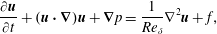(2.1)$$\begin{eqnarray}\displaystyle & \displaystyle \frac{\unicode[STIX]{x2202}\boldsymbol{u}}{\unicode[STIX]{x2202}t}+(\boldsymbol{u}\boldsymbol{\cdot }\unicode[STIX]{x1D735})\boldsymbol{u}+\unicode[STIX]{x1D735}p=\frac{1}{Re_{\unicode[STIX]{x1D6FF}}}\unicode[STIX]{x1D6FB}^{2}\boldsymbol{u}+f, & \displaystyle\end{eqnarray}$$

(2.2)$$\begin{eqnarray}\displaystyle & \displaystyle \unicode[STIX]{x1D735}\boldsymbol{\cdot }\boldsymbol{u}=0, & \displaystyle\end{eqnarray}$$

where $\boldsymbol{u}=(u,v,w)^{\text{T}}$ is the velocity vector, $p$ the pressure, $f$ a forcing term and $Re_{\unicode[STIX]{x1D6FF}}=U_{\infty }\unicode[STIX]{x1D6FF}/\unicode[STIX]{x1D708}$ is the Reynolds number based on the reference length $\unicode[STIX]{x1D6FF}$. In addition, the following boundary conditions are imposed. On the flat plate inflow boundary $\unicode[STIX]{x1D6E4}_{I}$, a Dirichlet condition sets the inflow velocity to a Blasius velocity profile $\boldsymbol{u}_{B}$. On the boundary $\unicode[STIX]{x1D6E4}_{W}$ composed of the flat plate surface and the pipe walls, the velocity is set to zero. At the pipe inflow $\unicode[STIX]{x1D6E4}_{P}$, a parabolic profile is imposed,

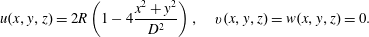(2.3a,b)$$\begin{eqnarray}u(x,y,z)=2R\left(1-4\frac{x^{2}+y^{2}}{D^{2}}\right),\quad v(x,y,z)=w(x,y,z)=0.\end{eqnarray}$$

On the outflow boundary $\unicode[STIX]{x1D6E4}_{O}$, standard outflow conditions are used,

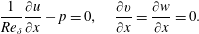(2.4a,b)$$\begin{eqnarray}\frac{1}{Re_{\unicode[STIX]{x1D6FF}}}\frac{\unicode[STIX]{x2202}u}{\unicode[STIX]{x2202}x}-p=0,\quad \frac{\unicode[STIX]{x2202}v}{\unicode[STIX]{x2202}x}=\frac{\unicode[STIX]{x2202}w}{\unicode[STIX]{x2202}x}=0.\end{eqnarray}$$

On the top boundary $\unicode[STIX]{x1D6E4}_{T}$, the conditions are

(2.5a-c)$$\begin{eqnarray}u=1,\quad v=0,\quad \frac{1}{Re_{\unicode[STIX]{x1D6FF}}}\frac{\unicode[STIX]{x2202}w}{\unicode[STIX]{x2202}z}-p=0.\end{eqnarray}$$

Finally, the domain is periodic in the spanwise direction.

Small perturbations $(\boldsymbol{u},p)^{\text{T}}$ about a steady-state solution $(\boldsymbol{U},P)^{\text{T}}$ of (2.1)–(2.4) are described by the linearized Navier–Stokes equations

(2.6)$$\begin{eqnarray}\displaystyle & \displaystyle \frac{\unicode[STIX]{x2202}\boldsymbol{u}}{\unicode[STIX]{x2202}t}+(\boldsymbol{U}\boldsymbol{\cdot }\unicode[STIX]{x1D735})\boldsymbol{u}+(\unicode[STIX]{x1D735}\boldsymbol{U})\boldsymbol{u}+\unicode[STIX]{x1D735}p=\frac{1}{Re_{\unicode[STIX]{x1D6FF}}}\unicode[STIX]{x1D6FB}^{2}\boldsymbol{u}, & \displaystyle\end{eqnarray}$$

(2.7)$$\begin{eqnarray}\displaystyle & \displaystyle \unicode[STIX]{x1D735}\boldsymbol{\cdot }\boldsymbol{u}=0. & \displaystyle\end{eqnarray}$$

The associated boundary conditions are

(2.8)$$\begin{eqnarray}\displaystyle \boldsymbol{u}=0\quad \text{on }\unicode[STIX]{x1D6E4}_{I}\cup \unicode[STIX]{x1D6E4}_{W}\cup \unicode[STIX]{x1D6E4}_{P}, & & \displaystyle\end{eqnarray}$$

(2.9a-c)$$\begin{eqnarray}\displaystyle u=0,\quad v=0,\quad \frac{1}{Re_{\unicode[STIX]{x1D6FF}}}\frac{\unicode[STIX]{x2202}w}{\unicode[STIX]{x2202}z}-p=0\quad \text{on }\unicode[STIX]{x1D6E4}_{T}, & & \displaystyle\end{eqnarray}$$

and either

(2.10)$$\begin{eqnarray}\boldsymbol{u}=0,\end{eqnarray}$$

or

(2.11a-c)$$\begin{eqnarray}\frac{1}{Re_{\unicode[STIX]{x1D6FF}}}\frac{\unicode[STIX]{x2202}u}{\unicode[STIX]{x2202}x}-p=0,\quad \frac{\unicode[STIX]{x2202}v}{\unicode[STIX]{x2202}x}=0,\quad \frac{\unicode[STIX]{x2202}w}{\unicode[STIX]{x2202}x}=0,\end{eqnarray}$$

on the outflow $\unicode[STIX]{x1D6E4}_{O}$.

The adjoint linearized Navier–Stokes equations

(2.12)$$\begin{eqnarray}\displaystyle & \displaystyle -\frac{\unicode[STIX]{x2202}\boldsymbol{u}^{\dagger }}{\unicode[STIX]{x2202}t}-(\boldsymbol{U}\boldsymbol{\cdot }\unicode[STIX]{x1D735})\boldsymbol{u}^{\dagger }+(\unicode[STIX]{x1D735}\boldsymbol{U})^{\text{T}}\boldsymbol{u}^{\dagger }+\unicode[STIX]{x1D735}p^{\dagger }=\frac{1}{Re_{\unicode[STIX]{x1D6FF}}}\unicode[STIX]{x1D6FB}^{2}\boldsymbol{u}^{\dagger }, & \displaystyle\end{eqnarray}$$

(2.13)$$\begin{eqnarray}\displaystyle & \displaystyle \unicode[STIX]{x1D735}\boldsymbol{\cdot }\boldsymbol{u}^{\dagger }=0, & \displaystyle\end{eqnarray}$$

are also used in the stability analysis along with the boundary conditions

(2.14)$$\begin{eqnarray}\displaystyle \boldsymbol{u}^{\dagger }=0\quad \text{on }\unicode[STIX]{x1D6E4}_{I}\cup \unicode[STIX]{x1D6E4}_{W}\cup \unicode[STIX]{x1D6E4}_{P}, & & \displaystyle\end{eqnarray}$$

(2.15a-c)$$\begin{eqnarray}\displaystyle u^{\dagger }=0,\quad v^{\dagger }=0,\quad \frac{1}{Re_{\unicode[STIX]{x1D6FF}}}\frac{\unicode[STIX]{x2202}w^{\dagger }}{\unicode[STIX]{x2202}z}-p^{\dagger }-Ww^{\dagger }=0\quad \text{on }\unicode[STIX]{x1D6E4}_{T}, & & \displaystyle\end{eqnarray}$$

and either

(2.16)$$\begin{eqnarray}\boldsymbol{u}^{\dagger }=0,\end{eqnarray}$$

or

(2.17a-c)$$\begin{eqnarray}\frac{1}{Re_{\unicode[STIX]{x1D6FF}}}\frac{\unicode[STIX]{x2202}u^{\dagger }}{\unicode[STIX]{x2202}x}-p^{\dagger }-Uu^{\dagger }=0,\quad \frac{1}{Re_{\unicode[STIX]{x1D6FF}}}\frac{\unicode[STIX]{x2202}v^{\dagger }}{\unicode[STIX]{x2202}x}-Uv^{\dagger }=0,\quad \frac{1}{Re_{\unicode[STIX]{x1D6FF}}}\frac{\unicode[STIX]{x2202}w^{\dagger }}{\unicode[STIX]{x2202}x}-Uw^{\dagger }=0,\end{eqnarray}$$

on the outflow $\unicode[STIX]{x1D6E4}_{O}$.

The homogeneous Dirichlet conditions at outflow (2.10) and (2.16) are only used for eigenvalue calculations. In this case, a sponge region is added at outflow to force the perturbations to zero. Its strength increases smoothly from 15 units upstream of the outflow to 5 units upstream, and is constant in the last five units. In all simulations a small sponge of total width of 3 units is also present at inflow.

3 Flow case and computational set-up

In the present work, a circular flush pipe is considered. The pipe is long enough to assume a parabolic profile far from the outlet even in the presence of the cross-flow. The coordinate origin is taken at the pipe centre on the flat plate. Following Ilak et al. (Reference Ilak, Schlatter, Bagheri and Henningson2012) and Peplinski, Schlatter & Henningson (Reference Peplinski, Schlatter, Henningson, Theofilis and Soria2015b), the reference length is taken to $\unicode[STIX]{x1D6FF}=D/3$, which was the boundary-layer displacement thickness at inflow $\unicode[STIX]{x1D6FF}_{0}^{\ast }$ in Ilak et al. (Reference Ilak, Schlatter, Bagheri and Henningson2012), situated at $x=-9.375$. The Blasius boundary-layer displacement thickness at the centre of the pipe exit is chosen to $\unicode[STIX]{x1D6FF}^{\ast }=1.0809$ (or $\unicode[STIX]{x1D6FF}^{\ast }/D=0.3603$), and the Reynolds number, unless stated otherwise, is set to $Re_{D}=495$.

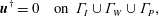
All simulations are performed with the spectral element code Nek5000 (Fischer, Lottes & Kerkemeier Reference Fischer, Lottes and Kerkemeier2008). The domain is represented in figure 1. A Blasius boundary-layer profile is imposed at the inflow boundary $\unicode[STIX]{x1D6E4}_{I}$. At the pipe inflow, a parabolic profile with top velocity $R$ is imposed. The pipe is 20 to 40 units (6.7 to 13.3 pipe diameters) long, which leaves enough distance for the pipe flow to adapt to the presence of the cross-flow. The simulation box width is 30 units, its height (pipe not included) 26 units and its length upstream of the pipe is 34 units. Downstream of the pipe, the length of the box varies from 125 to 200 units. The domain is assumed to be periodic in the spanwise direction. Boundary conditions are discussed in § 2.

In the spectral element method, the domain is partitioned into elements in which the solutions are approximated by polynomials of degree $N$. Thus, the polynomial order affects both the number of degrees of freedom in each element and the rate of spatial convergence of the numerical method. Here, the polynomial order is usually chosen at $N=7$. For convergence tests, $N=9$ is used. The domain with downstream length of $200$ units is comprised of 56 772 such elements. All three meshes used here only differ in their downstream length. A detail of the mesh near the pipe exit is shown in figure 3.

Figure 1.

Sketch of the computation domain.

The time integration is performed via third-order backwards difference for nonlinear simulations, and second order for linearized simulations. The time step varies between $3.0\times 10^{-3}$ and $3.5\times 10^{-3}$, for a maximum Courant–Friedrichs–Lewy number around 0.3.

4 Nonlinear simulations

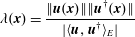
Peplinski et al. (Reference Peplinski, Schlatter and Henningson2015a) in their studies used Cartesian meshes and modelled the pipe flow with a non-homogeneous Dirichlet condition. In order to avoid discontinuities due to non-coincident points, the velocity distribution used was a parabolic profile smoothed with a super-Gaussian function. As a consequence, the shape of the velocity profile was different from the complete flow computed here, with a larger top velocity. In the present direct numerical simulations (DNS), the velocity profile at the pipe exit, shown in figure 2, appears significantly bent by the cross-flow, a feature that was also observed by Klotz et al. (Reference Klotz, Gumowski and Wesfreid2019). In particular, a stationary recirculation vortex can be seen in the upstream part of the pipe exit, consistent with the inner vortex described in Bidan & Nikitopoulos (Reference Bidan and Nikitopoulos2013).

A recirculation area is present behind the jet, nested between the counter-rotating vortices at their base.

Direct numerical simulations have been performed for different values of relevant parameters to find the border between the stable and unstable regions of the parameter space. At $Re_{D}=495$ and $R=0.35$, variations of 20 % of the boundary-layer displacement thickness $\unicode[STIX]{x1D6FF}^{\ast }$ had only a small effect on the decay rate of the perturbations measured in a direct simulation and the flow remained clearly stable in both cases. For $\unicode[STIX]{x1D6FF}^{\ast }/D=0.2882$, the growth rate of the oscillations in the linear phase of the DNS is approximately $\unicode[STIX]{x1D70E}=-0.0064$, compared to $\unicode[STIX]{x1D70E}=-0.0082$ at $\unicode[STIX]{x1D6FF}^{\ast }/D=0.4324$. We do not consider further this dependency in our work. For details of the stability analysis see § 5.

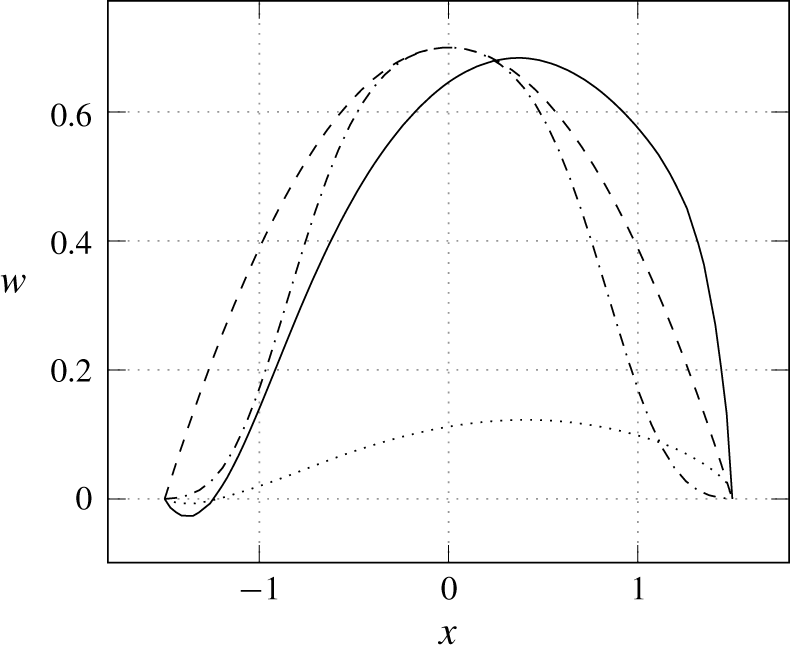
Figure 2.

Different pipe vertical velocity profiles at the pipe exit. Current DNS (——), parabolic profile (– – –), Ilak et al. (Reference Ilak, Schlatter, Bagheri and Henningson2012) (– ⋅ – ⋅ –). The streamwise velocity in the current DNS is also represented ($\cdots \cdots$).

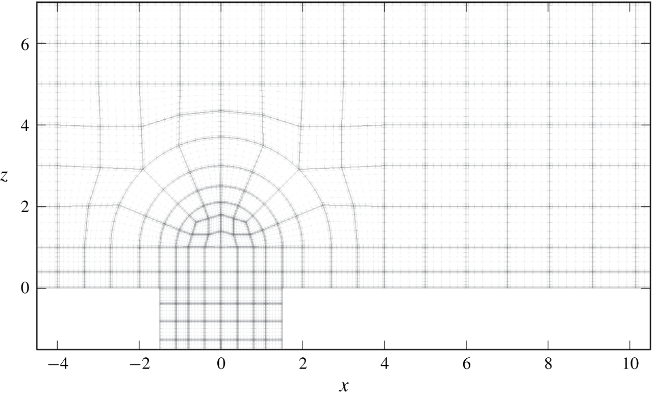
Figure 3.

Detail of the mesh in the vicinity of the pipe exit in the symmetry plane. The thick lines denote the spectral element boundaries. The thin lines represent the computation grid inside each element.

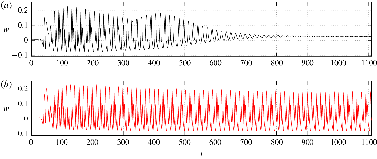
Figure 4.

Wall-normal velocity at the location ($x=25$, $y=0$, $z=4$) for (a) $R=0.35$, and (b) $R=0.375$.

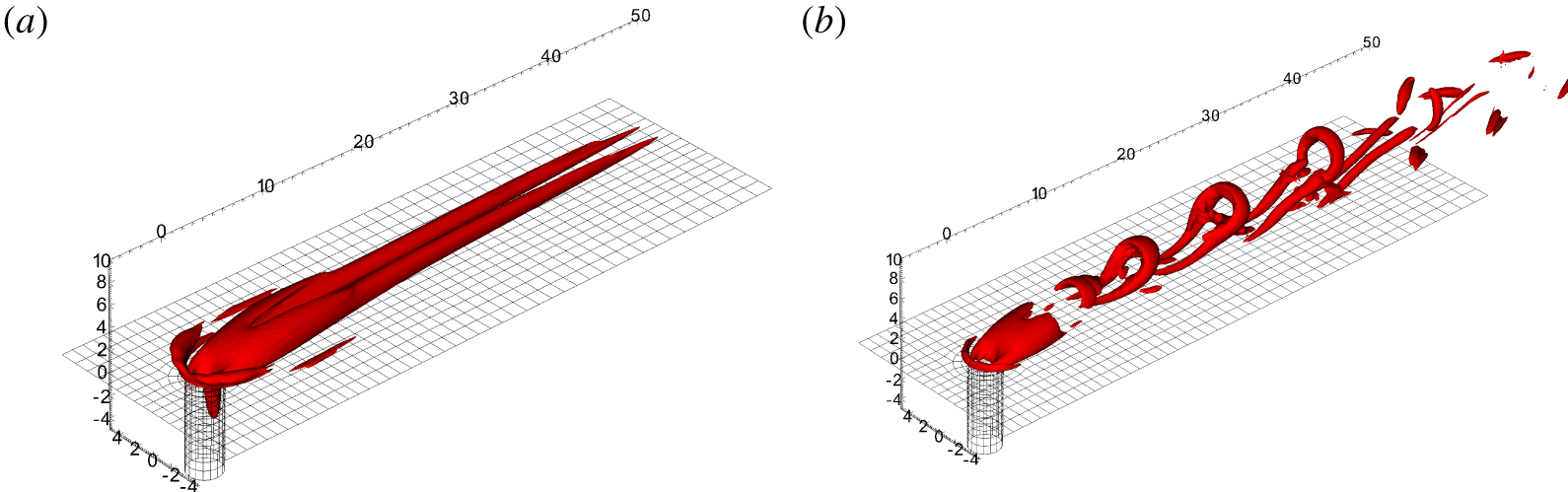
Figure 5.

Contours of $\unicode[STIX]{x1D706}_{2}$ for (a) a stable and (b) an unstable jet.

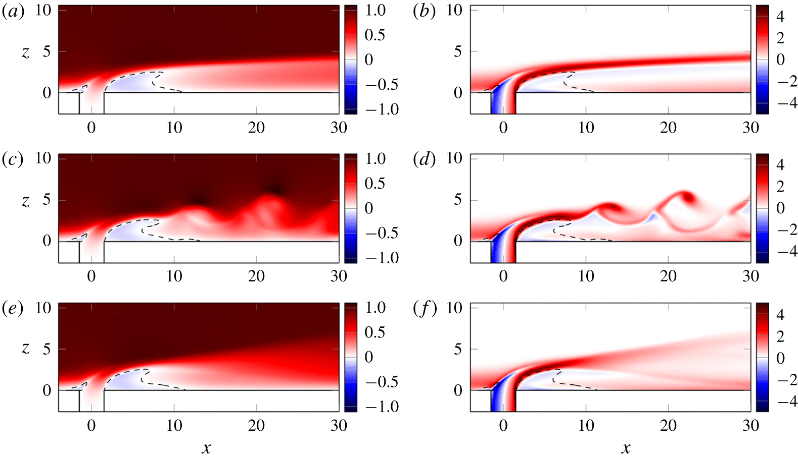
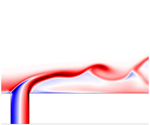
Figure 6.

Streamwise velocity (a,c,e) and scaled spanwise vorticity $D\unicode[STIX]{x1D714}_{y}$ (b,d,f) in the symmetry plane. (a,b) Steady flow at $R=0.35$; (c,d) instantaneous flow at $R=0.4$; (e,f) time-averaged flow at $R=0.4$. The dashed lines delimit the corresponding areas of negative streamwise velocity.

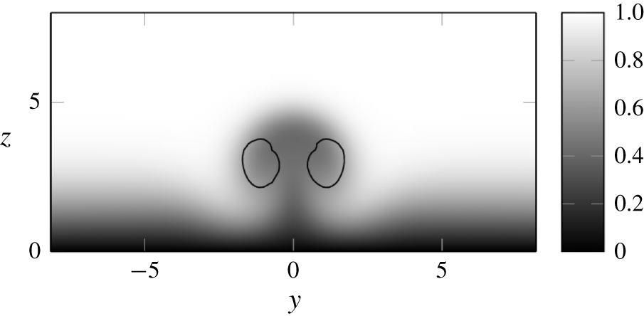
Figure 7.

Streamwise velocity in the wake of the steady jet ($R=0.35$) in the plane ($x$, $y$) at $x=40$. The contours of $\unicode[STIX]{x1D706}_{2}=-0.0003$ in black indicate the position of the counter-rotating vortices.

At very low velocity ratios, the jet converges to a steady state. Once the velocity ratio is increased above some critical value, a bifurcation to a limit cycle occurs. Figure 4 shows the variation of the velocity in the wake of the jet for a stable and an unstable velocity ratio. The initial condition for those simulations is a Blasius flow with zero velocity inside the pipe. The jet forms rapidly and starts to oscillate due to the instability. The oscillations are small at the pipe exit and grow downstream. In figure 4 the velocity is measured just below the trajectory of the centres of the hairpin vortices, which is why higher frequencies are present when the amplitude of the oscillations is large.

In figures 5(a) and 5(b), the flow fields corresponding to a stable and unstable jet are shown using the $\unicode[STIX]{x1D706}_{2}$ criterion (Jeong & Hussain Reference Jeong and Hussain1995). The main feature of the steady jet is a pair of counter-rotating vortices extending far downstream. They significantly lift the boundary layer (figure 7), producing strong streaks in the wake. The lifting of the boundary layer also concentrates the spanwise vorticity in a thin shear layer along the jet streamlines. The horseshoe vortex (Kelso & Smits Reference Kelso and Smits1995), surrounding the base of the jet, is also clearly visible in figure 5(a). In figure 6 the streamwise velocity and spanwise vorticity in the symmetry plane are shown for both the stable and the unstable case. Those figures are qualitatively similar to the experimental results by Klotz et al. (Reference Klotz, Gumowski and Wesfreid2019, figure 7). They show the same distinct shape of the recirculation area behind the jet and below the shear layer. In the stable case, we observe a thin shear layer along the jet trajectory. In the unstable case, hairpin vortices are shed from the shear layer above the recirculation area. The regions upstream and up to the recirculation area are barely affected by the unsteadiness.

In the periodic case at $R=0.375$, the frequency is close to $f=0.068$ corresponding to a Strouhal number ${S_{t}}_{D}=fD/U_{\infty }=0.205$. For the stable jet at $R=0.35$, a Fourier transform of the time signal (figure 4a) shows a peak at a very close frequency,$f=0.066$ (${S_{t}}_{D}=0.20$).

A summary of the nonlinear simulations is presented in figure 8. For reference, results of some other works are presented there too. All unstable cases studied here display the same type of instability consisting of hairpin vortices, although different types of instabilities are present with parameters further away from this neutral curve (see for example Regan & Mahesh (Reference Regan and Mahesh2017)). As expected and seen in figure 8, the jet appears more stable at low Reynolds numbers. At $Re_{D}=495$ and $\unicode[STIX]{x1D6FF}^{\ast }/D=0.3603$, the stability limit is found slightly above $R=0.35$ with the pipe fully meshed. The neutral curve found here is close to the experimental results from Klotz et al. (Reference Klotz, Gumowski and Wesfreid2019) who studied a similar range of parameters, although in their experiments the boundary layer was thinner, with $\unicode[STIX]{x1D6FF}^{\ast }/D$ ranging from 0.26 to 0.3. A comparison with a very low velocity ratio case in Cambonie & Aider (Reference Cambonie and Aider2014), at $R=0.16$ is also made. This point, located significantly below our neutral curve, was reported unstable.

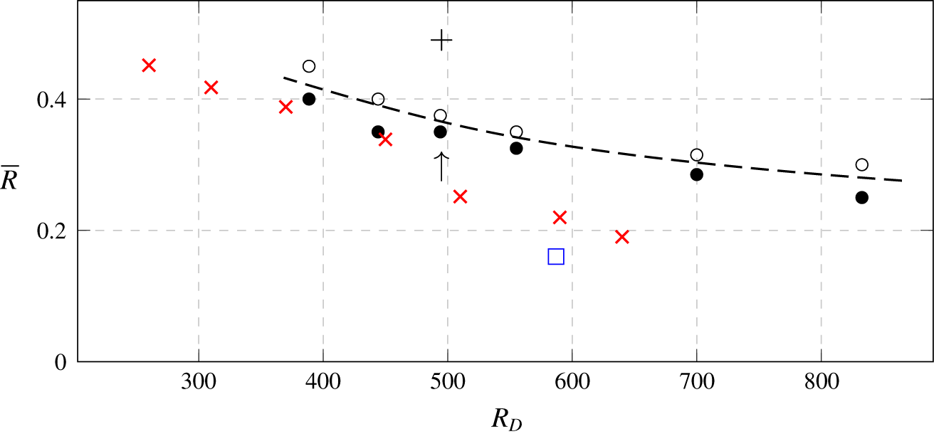
Figure 8.

Neutral stability curve at $\unicode[STIX]{x1D6FF}^{\ast }/D=0.3603$. The stable cases, converging to a steady state, are shown by filled circles. The open circles are unsteady cases, converging to periodic limit cycles. The dashed line indicates the approximate location of the neutral curve. The red crosses are the critical velocity ratios found experimentally by Klotz et al. (Reference Klotz, Gumowski and Wesfreid2019) for slightly thinner boundary layers, and the blue square is the case number 7 in Cambonie & Aider (Reference Cambonie and Aider2014). The plus symbol at the top indicates the previous critical velocity ratio estimated by Peplinski et al. (Reference Peplinski, Schlatter and Henningson2015a). The arrow indicates $Re_{D}=495$, where the stability analysis is performed in § 5.

5 Stability analysis

For incompressible flows, there is no evolution equation for the pressure, which only acts as a Lagrange multiplier keeping the divergence-free conditions (2.2), (2.7) and (2.13) satisfied. As a consequence, equations (2.6)–(2.11) and the associated boundary conditions can be written as the dynamical system

(5.1)$$\begin{eqnarray}\frac{\unicode[STIX]{x2202}\boldsymbol{u}}{\unicode[STIX]{x2202}t}=\boldsymbol{A}\boldsymbol{u},\end{eqnarray}$$

where $\boldsymbol{A}$ is the linearized Navier–Stokes operator. The adjoint linearized Navier–Stokes operator $\boldsymbol{A}^{\dagger }$ can be defined in the same way from (2.12)–(2.17).

We note the energy inner product $\langle \boldsymbol{u},\boldsymbol{v}\rangle _{E}=\int _{\unicode[STIX]{x1D6FA}}\boldsymbol{u}\boldsymbol{\cdot }\boldsymbol{v}\,\text{d}\unicode[STIX]{x1D6FA}$, where $\unicode[STIX]{x1D6FA}$ denotes the computational domain, and $\Vert ~\Vert _{E}$ its associated norm.

5.1 Eigenspectra

In order to determine the eigenmodes of $\boldsymbol{A}$, the eigenvalue problem $\exp (\unicode[STIX]{x1D70F}\boldsymbol{A})\boldsymbol{u}=\text{i}\unicode[STIX]{x1D714}\boldsymbol{u}$ is solved using the implicitly restarted Arnoldi method (Lehoucq, Sorensen & Yang Reference Lehoucq, Sorensen and Yang1998) by time stepping the equations (2.6)–(2.7) in Nek5000 for a chosen time $\unicode[STIX]{x1D70F}$. This integration time is selected to be between one tenth and one fifth of the period of the oscillations observed in DNS in order to avoid aliasing. The eigenvalues $(\unicode[STIX]{x1D706}_{i})$ of $\boldsymbol{A}$ are then recovered with

(5.2)$$\begin{eqnarray}\unicode[STIX]{x1D706}_{i}=\frac{\ln \unicode[STIX]{x1D707}_{i}}{\unicode[STIX]{x1D70F}},\end{eqnarray}$$

where $(\unicode[STIX]{x1D707}_{i})$ are the computed eigenvalues of $\exp (\unicode[STIX]{x1D70F}\boldsymbol{A})$. The Krylov space size is chosen to 120 vectors and the algorithm is iterated until at least 20 eigenvalues are converged with residuals below $10^{-6}$. In addition, for one run a Krylov space of size 200 was used in order to converge 50 eigenvalues (figure 9).

The base flows are computed using selective frequency damping (Åkervik et al. Reference Åkervik, Brandt, Henningson, Hœpffner, Marxen and Schlatter2006). It consists of forcing the flow to a low-pass filtered version of itself. Here, the forcing coefficient is $\unicode[STIX]{x1D712}=0.0333$ and the filter width is $\unicode[STIX]{x1D6E5}=30$, or approximately twice the observed period of the oscillations, so as to damp satisfactorily the oscillations without slowing down the convergence to the steady state too much. The instability being oscillatory, this method was found to be effective. The maximum of the difference between the instantaneous velocity and the filtered velocity was decreased below $10^{-11}$.

At $R=0.35$ (figure 9), the system is found to be linearly stable. Besides a number of ‘box modes’ (modes composed of structures extending up to the downstream box boundary and dependant on the box size), a pair of complex conjugated eigenvalues is found below the real axis. At $R=0.4$ (figure 10), this pair of eigenvalues has moved significantly above the real axis, confirming that the jet has undergone a Hopf bifurcation. To investigate the effects of box size and resolution, a series of computations were performed. The results are also documented in figures 9 and 10. For both of these velocity ratios the effect of the box length is clearly visible. The frequency of the dominant mode was predicted well in all cases but not its growth rate. It was found that a downstream length of 125 units is not sufficient to capture properly even the most unstable mode. The variations in the growth rate of the dominant mode decayed with increasing domain size. The differences between the downstream length of 150 and 200 units were small enough (especially for the unstable case) to assume the dominant mode being converged, therefore a downstream length of 200 units was chosen for the remaining computations.

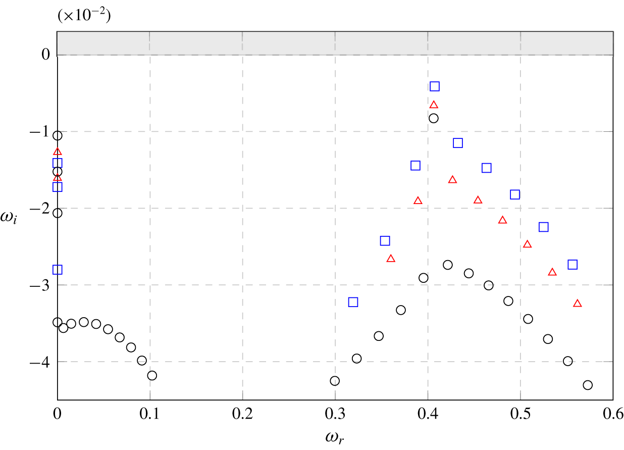
Figure 9.

Spectra at $R=0.35$ with polynomial order $N=7$ and tolerances $\unicode[STIX]{x1D716}=10^{-14}$ for box length 125 (▫ – blue), 150 (▵ – red) and 200 (○).

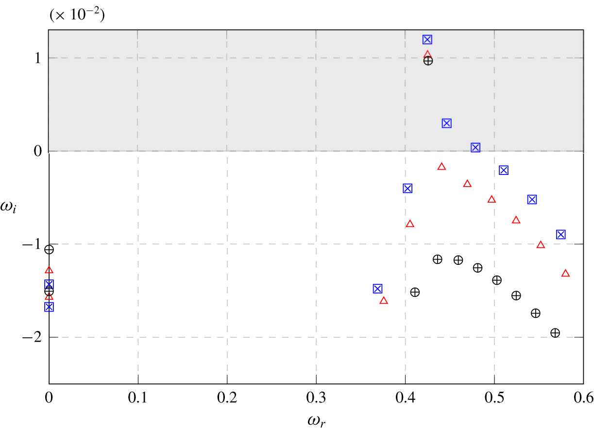
Figure 10.

Spectra at $R=0.4$ with polynomial order $N=7$ and tolerances $\unicode[STIX]{x1D716}=10^{-14}$ for direct equations with box length 125 (▫ – blue), 150 (▵ – red) and 200 (○) and adjoint equations with length 125 (× – blue) and 200 ($+$).

Another set of computations was performed to check the sensitivity of the stability analysis to the mean flow accuracy. Here, both the momentum equations and the divergence-free equation are solved iteratively at each time step. As a consequence, the action of the operator is not solved to machine precision, but within a user-specified tolerance $\unicode[STIX]{x1D716}$. This can be seen as solving a slightly different operator differing from the actual linearized Navier–Stokes operator by a small perturbation of the order of the specified tolerance. The Ritz values returned by the code are therefore $\unicode[STIX]{x1D716}$-pseudoeigenvalues of the operator rather than proper eigenvalues. The excellent agreement between the direct and adjoint eigenspectra in figure 10 with $\unicode[STIX]{x1D716}=10^{-14}$ shows that the 20 requested eigenvalues are numerically converged. This is further confirmed by the excellent agreement between spectra obtained by computing both the base flow and the perturbations at polynomial orders $N=7$ and $N=9$ (not shown here). If the residual tolerance for both equations is relaxed to $\unicode[STIX]{x1D716}=10^{-10}$, only the most unstable pair of eigenvalues can be approximated (figure 11). The other eigenvalues shift significantly when numerical parameters are modified. Here, the direct and adjoint spectra are represented for two different polynomial orders, $N=7$ and $N=9$. The error for the unstable eigenvalue compared to the converged spectra with $\unicode[STIX]{x1D716}=10^{-14}$ is of the order of $10^{-3}$ for the direct eigenspectra, and $10^{-4}$ for the adjoint eigenspectra. The damping of the branch of convective modes is also better approximated with the adjoint equations than with the direct ones.

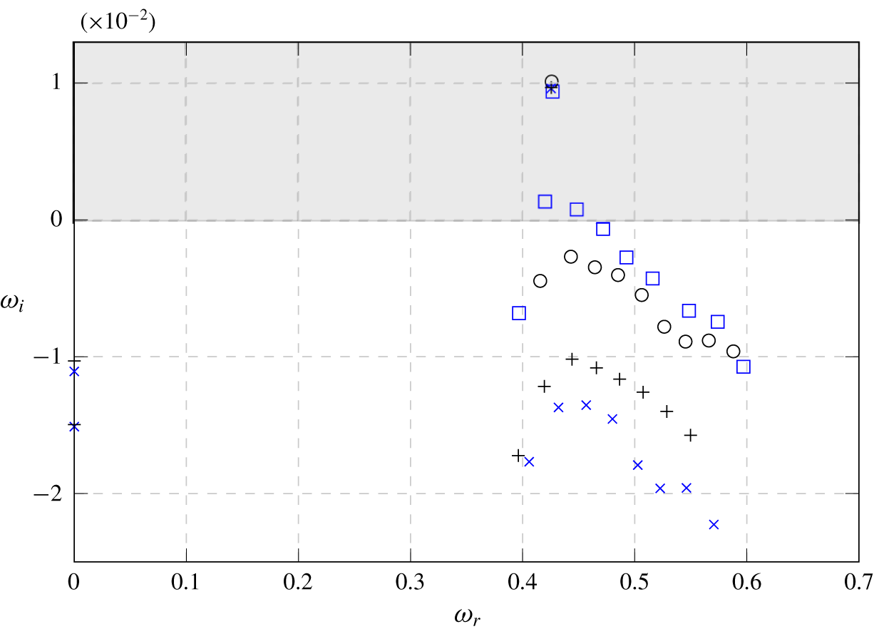
Figure 11.

Spectra at $R=0.4$ and box length 200 with tolerances $\unicode[STIX]{x1D716}=10^{-10}$ for the direct equations at $N=7$ (▫ – blue) and $N=9$ (○), and the adjoint equations at $N=7$ (× – blue) and $N=9$ ($+$).

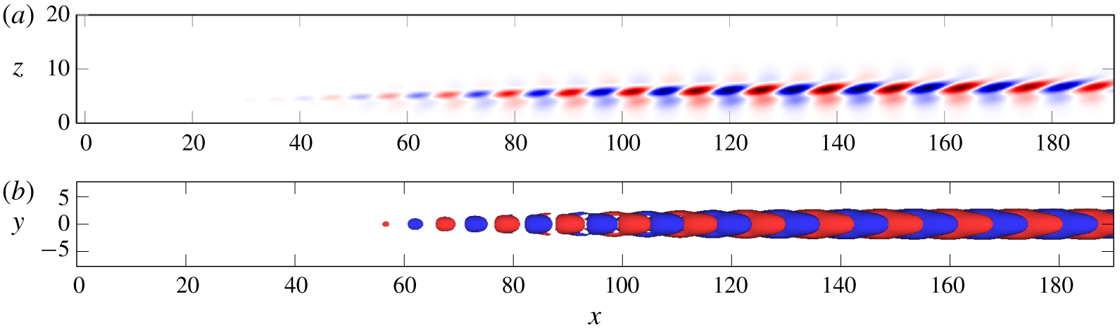
Figure 12.

Real part of $\hat{u}$ in the symmetry plane (a) and contours of $\text{Re}(\hat{u} )=\pm 0.008$ (b) for the most unstable direct mode at $R=0.35$.

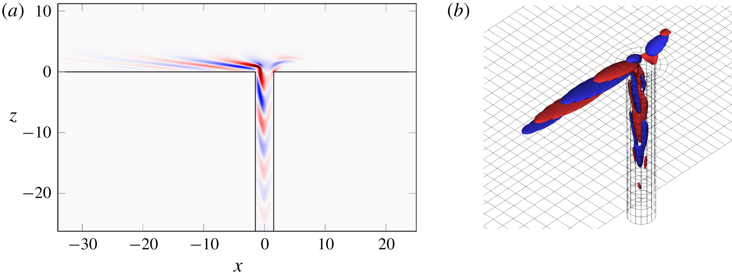
Figure 13.

Real part of $\hat{u} ^{\dagger }$ in the symmetry plane (a) and contours of $\text{Re}(\hat{u} ^{\dagger })=\pm 0.008$ (b) for the most unstable adjoint mode at $R=0.35$.

The real part of the eigenvector associated with the most unstable pair of eigenvalues and their corresponding adjoint modes are represented in figures 12 and 13, respectively. The amplitude of the direct mode is the most significant far downstream from the pipe exit, whereas the adjoint mode is large upstream and in the direct vicinity downstream of the pipe. As a consequence, the direct and adjoint modes are close to orthogonal, which is a measure of the non-normality of the operator. The degree of non-normality increases with the size of the box, as the direct eigenvector continues to grow downstream. For a downstream length of $L_{x}=200$ with $R=0.4$, it is particularly high, with

(5.3)$$\begin{eqnarray}\frac{|\langle \boldsymbol{u},\boldsymbol{u}^{\dagger }\rangle _{E}|}{\Vert \boldsymbol{u}\Vert _{E}\Vert \boldsymbol{u}^{\dagger }\Vert _{E}}<10^{-11}.\end{eqnarray}$$

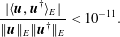
The wavemaker (Giannetti & Luchini Reference Giannetti and Luchini2007), defined as

(5.4)$$\begin{eqnarray}\unicode[STIX]{x1D706}(\boldsymbol{x})=\frac{\Vert \boldsymbol{u}(\boldsymbol{x})\Vert \Vert \boldsymbol{u}^{\dagger }(\boldsymbol{x})\Vert }{|\langle \boldsymbol{u},\boldsymbol{u}^{\dagger }\rangle _{E}|}\end{eqnarray}$$

is represented in figure 14. Its location very close to the pipe exit, where the amplitude of the direct eigenvector is several orders of magnitude smaller than its maximum amplitude, may explain the high sensitivity of the spectrum to solver tolerance.

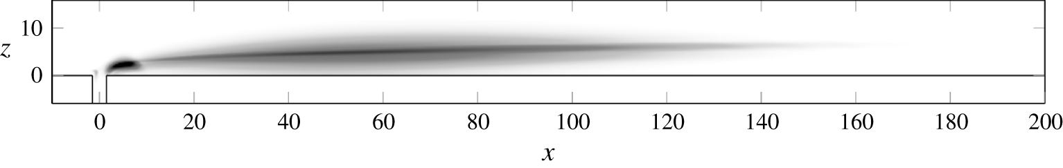
Figure 14.

Wavemaker for the most unstable mode at $R=0.35$.

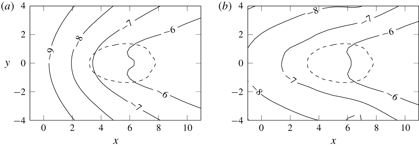
Figure 15.

Contours of the amplitude of $\log _{10}\Vert \hat{\boldsymbol{u}}(\boldsymbol{x})\Vert$ (solid lines) for the most unstable direct mode at $R=0.35$ in the plane $z=2.4$, where the wavemaker is the largest, with solver tolerances of (a) $\unicode[STIX]{x1D716}=10^{-14}$, and (b) $\unicode[STIX]{x1D716}=10^{-10}$. The dashed line is the contour of the wavemaker amplitude $\unicode[STIX]{x1D706}(\boldsymbol{x})=1000$.

Indeed, with tolerances of $10^{-10}$, the amplitude of the direct eigenvector for the most unstable mode differs significantly from the more accurate case with tolerances of $10^{-14}$, as shown in figures 15(a) and 15(b). In this area, the amplitude of the direct eigenvector appears to be too small to be resolved by the solver if the tolerances are not tight enough. This issue with $\unicode[STIX]{x1D716}=10^{-10}$ worsens when the downstream length of the box is increased, since the eigenvector grows downstream and the ratio between the maximum amplitude and the amplitude in the wavemaker increases. The vectors computed in the Arnoldi iterations are normalized to 1 in energy, and as the box length is increased, the normalized value around the wavemaker decreases below the solver tolerances. The adjoint eigenvectors do not exhibit such a large growth in space, which may explain why in figure 11 the adjoint eigenvalues are closer to the converged values. This phenomenon is similar to the results reported on the Batchelor vortex (Heaton, Nichols & Schmid Reference Heaton, Nichols and Schmid2009). On the other hand, because of the very small denominator in (5.4), the wavemaker remains very large far downstream in the wake, which requires the simulation box length to be long enough to fully capture the dynamics of the instability.

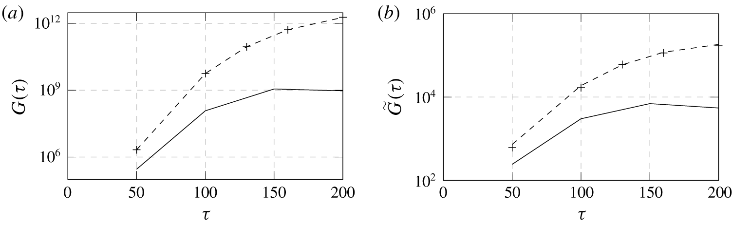
Figure 16.

(a) Optimal transient growth in energy, and (b) the growth in maximum amplitude associated with the optimal perturbations for energy growth, for $R=0.3$ (——) and $R=0.35$ (– – –) with a downstream box length of 200 units, and $R=0.35$ with a downstream length of 150 ($+$).

5.2 Noise amplification

Due to the strong non-normality of the operator responsible for the numerical sensitivity of the spectrum, it can be more useful to focus instead on transient growth. The optimization of the initial disturbance giving the largest transient growth at a fixed time avoids the numerical sensitivity issues found with the modal analysis since it involves self-adjoint operators. Physically, this might be related to what can be measured in experiments with finite amounts of noise.

Optimal disturbances maximizing energy growth at different times $\unicode[STIX]{x1D70F}$ are computed here with the singular value decomposition of the operator $\exp (\unicode[STIX]{x1D70F}\boldsymbol{A})$ (see Monokrousos et al. (Reference Monokrousos, Åkervik, Brandt and Henningson2010) for details of the implementation). Starting from a random vector $u_{0}$, the direct Navier–Stokes equations are integrated by time stepping from the initial time to the time $\unicode[STIX]{x1D70F}$. Then using the normalized result as the initial condition, the adjoint equations are integrated from time $\unicode[STIX]{x1D70F}$ to the initial time (backwards in time). After approximately three iterations, the result is close to the eigenvector associated with the largest eigenvalue $\unicode[STIX]{x1D707}_{o}(\unicode[STIX]{x1D70F})$ of $\exp (\unicode[STIX]{x1D70F}\boldsymbol{A}^{\dagger })\exp (\unicode[STIX]{x1D70F}\boldsymbol{A})$. The maximum transient growth at horizon $\unicode[STIX]{x1D70F}$ is then $G(\unicode[STIX]{x1D70F})=\sqrt{\unicode[STIX]{x1D707}_{0}(\unicode[STIX]{x1D70F})}$.

Optimal transient growth at different times is shown in figure 16(a) for two stable velocity ratios. For $R=0.3$, where the flow is clearly linearly stable, transient amplifications of the order of $10^{9}$ in energy are possible. For $R=0.35$ this value is over $10^{12}$. Amplification in velocity amplitude may be a more relevant measure for predicting transition to turbulence. Figure 16(b) shows the ratio of maximum response amplitude to maximum initial perturbation amplitude,

(5.5)$$\begin{eqnarray}\tilde{G}(\unicode[STIX]{x1D70F})=\frac{\Vert \text{exp}(\unicode[STIX]{x1D70F}\boldsymbol{A})\boldsymbol{u}_{0}\Vert _{\infty }}{\Vert \boldsymbol{u}_{0}\Vert _{\infty }},\end{eqnarray}$$

obtained with the same data, which gives a lower bound to the maximum amplification in amplitude. The ratio of disturbance amplitudes for $R=0.3$ can be of the order of $10^{4}$ and for $R=0.35$ of the order of $10^{5}$. However, Peplinski et al. (Reference Peplinski, Schlatter and Henningson2015a) showed that nonlinear effects could substantially decrease the amplification of this optimal perturbation.

Those simulations do not involve any eigenvalue computations and the perturbation fields, even at time horizon $\unicode[STIX]{x1D70F}=200$, are contained well within the long box with downstream length 200, thus the length of the box should only have a negligible effect. In order to confirm this, the optimal transient growth has also been computed with a downstream length of 150 units. The difference in energy growth is smaller than 1 %. This shows that even though transient growth is related to the superposition of non-orthogonal eigenvectors with different decay rates, the non-modal computation of optimal transient growth is more robust to changes in the size of the domain than eigenvalue calculations. For different box sizes, the same transient growth behaviour can be expressed in a different superposition of different eigenmodes. A similar observation was already made by Ehrenstein & Gallaire (Reference Ehrenstein and Gallaire2008) for a two-dimensional detached boundary-layer flow, even though they explicitly computed the optimal perturbation as a superposition of eigenvectors.

In order to estimate what response can be expected from noise that is not optimized to yield the maximum transient growth, further nonlinear simulations are run at $R=0.3$ and $R=0.35$ by adding random noise of amplitude 1 % in a box of coordinates $x\in [-20,10]$, $y\in [-10,10]$, $z\in [-10,10]$ at a time $t=t_{0}$. The noise has no particular spatial structure; a random value between $-0.01$ and 0.01 is added to all three velocity components at each grid point.

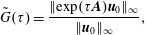
The response at coordinates $x=25$, $y=0$, $z=4$ is plotted in figure 17. At $R=0.3$, a train of hairpin vortices, displayed in figure 17(c), is generated before the flow quickly goes back to a steady state. At $R=0.35$, the amplitude of the response is larger and the shedding of hairpin vortices is sustained for a much longer time. This indicates that, in experiments, transient growth may still be an issue, but if the turbulence intensity is small enough or if its spatial structure has a very small projection on the optimal perturbation it could be possible to obtain a steady flow.

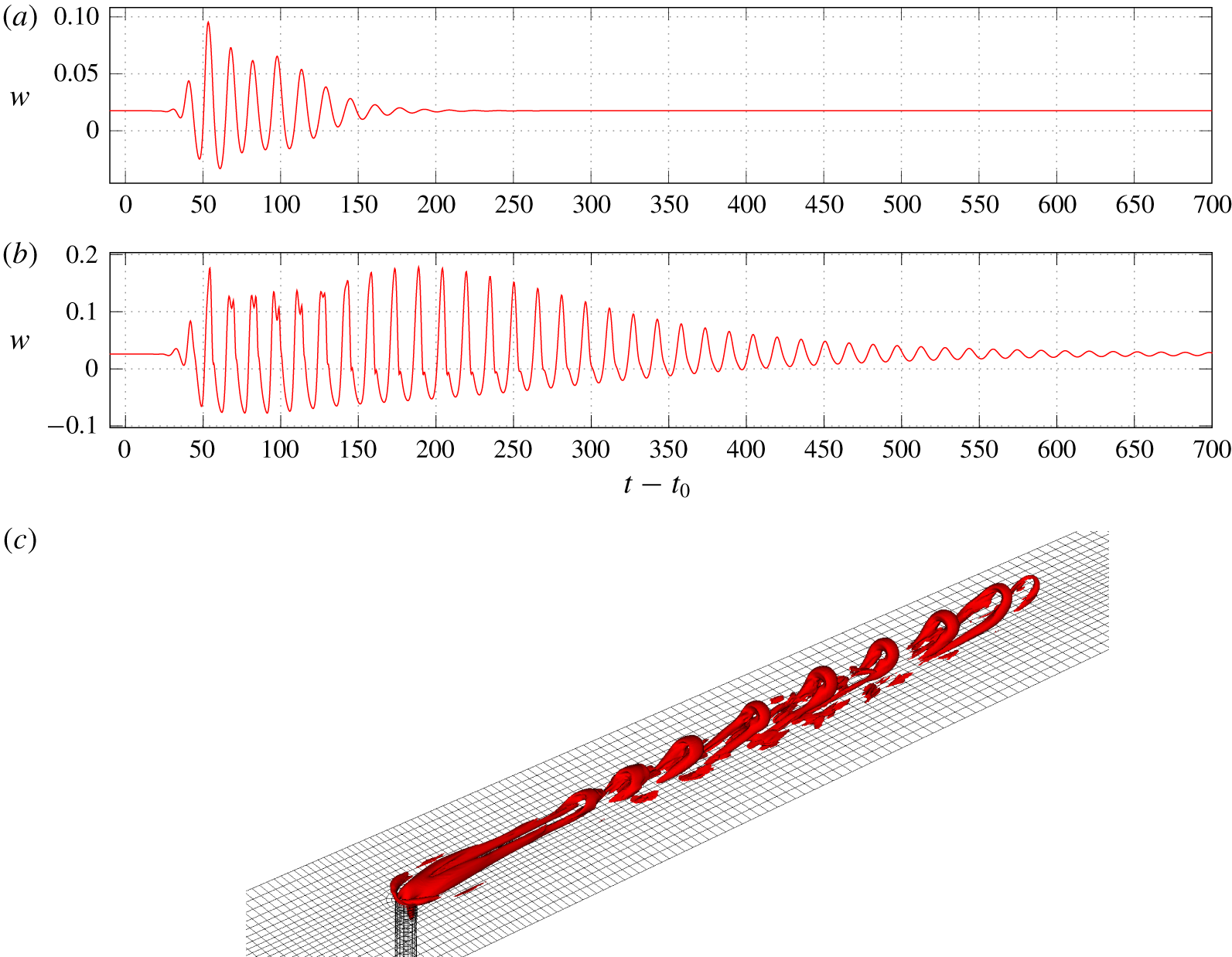
Figure 17.

Wall-normal velocity at the location ($x=25$, $y=0$, $z=4$) for (a) $R=0.3$, and (b) $R=0.35$, with noise of amplitude 1 % added at time $t_{0}$. The response at $R=0.3$ and time $t-t_{0}=168.5$ is shown in (c).

5.3 Wave packet analysis

A wave packet analysis is conducted in a linearized framework by evolving an initial disturbance localized around the pipe exit. The disturbance is chosen as the optimal disturbance for the time horizon $\unicode[STIX]{x1D70F}=160$ for the jet at $R=0.35$ computed in § 5.2 in order to achieve near optimal growth. The leading edge of the wave packet eventually leaves the domain at $t\simeq 280$, after which the perturbation flow is dominated by the leading mode and the perturbation energy, plotted in figure 18, evolves exponentially according to its growth rate. This method was applied to the velocity ratios $R=0.35$, $0.375$ and $0.4$. It displays a very good agreement with the eigenvalues found in § 5.1 for $R=0.35$ and $R=0.4$ and shows that the jet is already globally unstable at $R=0.375$, with a growth rate of 0.00288. The critical velocity ratio can be estimated at $R_{c}\simeq 0.368$ via a quadratic interpolation of these results. This analysis allows the growth rate of the most unstable mode to be determined more quickly than by computing eigenvalues of the linearized operator, and does not suffer from sensitivity induced by non-normality effects.

The propagation of the wave packet at $R=0.35$ is shown in more detail in figure 19. The square root of the energy in $y$–$z$ planes is plotted as a function of $(x-x_{0})/t$, where $x_{0}=-1.5$ is approximately the centre of gravity of the initial perturbation. It shows that the wave packet propagates at approximately half the free-stream velocity and accelerates as it moves downstream. The local energy at $(x-x_{0})/t=0$ initially decreases because of transient effects, but slowly increases at long times as the exponential growth phase is reached, consistent with the growth rate.

Figure 18.

Normalized energy norm response to a wave packet for $R=0.35$ (——),$R=0.375$ (– – –) and $R=0.4$ (– ⋅ – ⋅ –). The light straight lines represent exponential evolution with the rates found through eigenvalue analysis for $R=0.35$ and $R=0.4$.

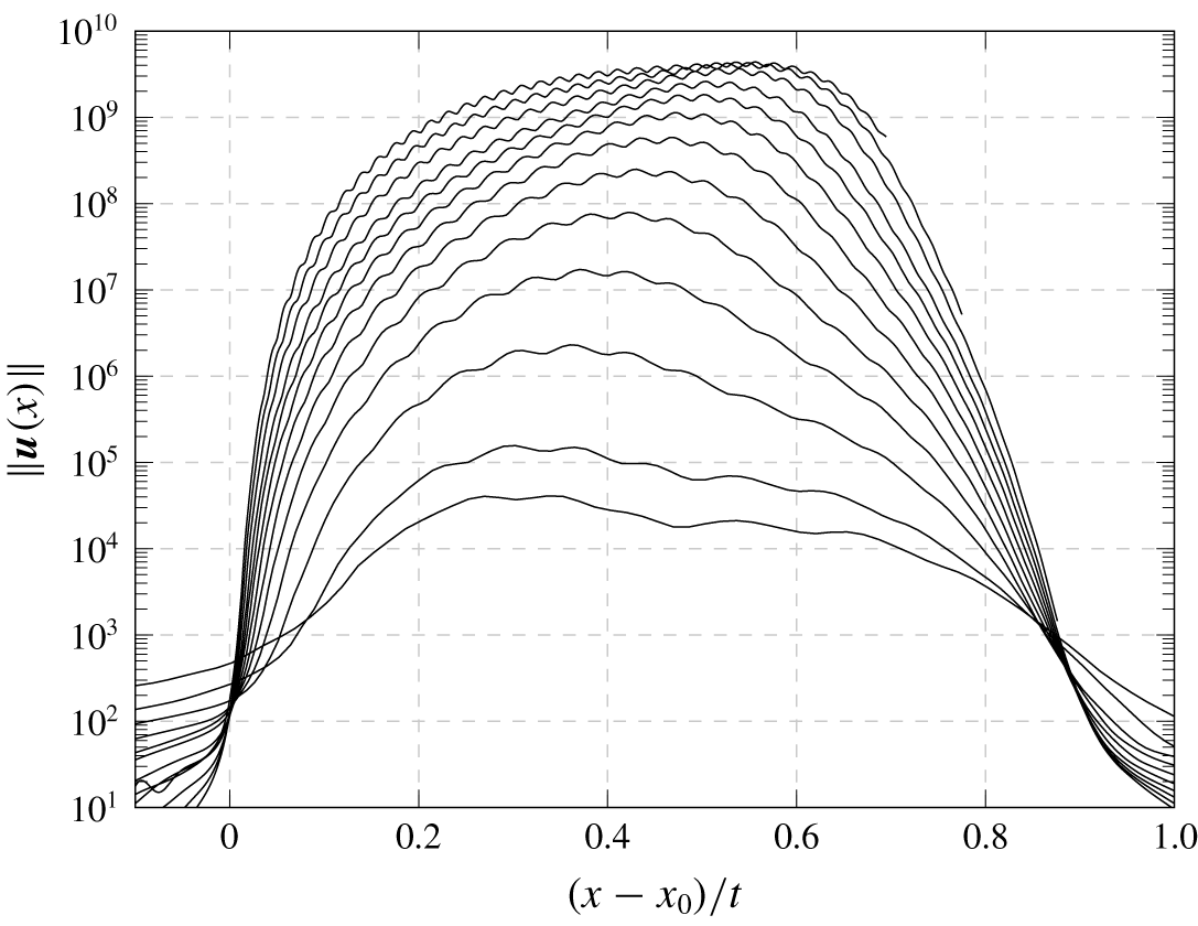
Figure 19.

Energy integrated in the $y$–$z$ plane as a function of the velocity $(x-x_{0})/t$ for $R=0.375$ at times $t=30$, 40, 60, 80, 100, 120, 140, 160, 180, 200, 230, 260 and 290, from bottom to top.

5.4 Optimal forcing

In order to further study the sensitivity of this flow, we compute the optimal periodic forcing. The algorithm introduced in Monokrousos et al. (Reference Monokrousos, Åkervik, Brandt and Henningson2010) to compute optimal forcing was implemented in Nek5000. This method can be seen as computing the largest singular value of the operator $(\boldsymbol{A}-\text{i}\unicode[STIX]{x1D714}\boldsymbol{I})^{-1}$. The largest eigenvalue $\unicode[STIX]{x1D707}_{0}(\unicode[STIX]{x1D714})$ and associated eigenvector $\boldsymbol{f}_{0}(\unicode[STIX]{x1D714})$ of the positive self-adjoint operator $((\boldsymbol{A}-\text{i}\unicode[STIX]{x1D714}\boldsymbol{I})^{-1})^{\dagger }(\boldsymbol{A}-\text{i}\unicode[STIX]{x1D714}\boldsymbol{I})^{-1}$ are computed through time stepping using power iterations. In this process, the response to the optimal forcing,

(5.6)$$\begin{eqnarray}\boldsymbol{r}_{0}(\unicode[STIX]{x1D714})=(\boldsymbol{A}-\text{i}\unicode[STIX]{x1D714}\boldsymbol{I})^{-1}\boldsymbol{f}_{0}(\unicode[STIX]{x1D714})\end{eqnarray}$$

is also obtained. The resolvent norm is then determined by

(5.7)$$\begin{eqnarray}{\mathcal{R}}(\unicode[STIX]{x1D714})=\Vert (\boldsymbol{A}-\text{i}\unicode[STIX]{x1D714}\boldsymbol{I})^{-1}\Vert =\sqrt{\unicode[STIX]{x1D707}_{0}(\unicode[STIX]{x1D714})}.\end{eqnarray}$$

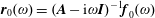
The resolvent norm and optimal forcing are computed at different angular frequencies for the velocity ratio $R=0.3$. The boundary conditions (2.17) and (2.11) are used here so that the response can leave the domain if it extends too far away. This is the case at low frequencies in particular. Around the frequency of the instability, $\unicode[STIX]{x1D714}\simeq 0.4$, the forcing (respectively response) has structures similar to the least stable adjoint (respectively direct) eigenmodes (figures 20 and 21). At low frequencies, the optimal forcing and response become sinuous, resulting in a lateral oscillation of the wake very far downstream.

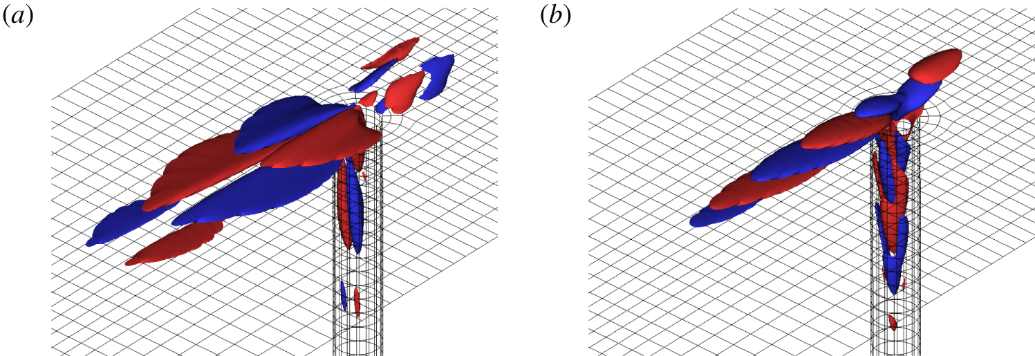
Figure 20.

Structure of streamwise component of the optimal forcing at $R=0.3$ and (a) $\unicode[STIX]{x1D714}=0.2$ and (b) $\unicode[STIX]{x1D714}=0.4$.

Figure 21.

Structure of streamwise component of the response to optimal forcing at $\unicode[STIX]{x1D714}=0.2$ (a) and $\unicode[STIX]{x1D714}=0.4$ (b).

The values of the resolvent norm are shown in figure 22. A simulation with polynomial order $N=9$ at $\unicode[STIX]{x1D714}=0.4$ shows excellent agreement (within 0.01 %) with the value found at $N=7$, confirming that the grid resolution is sufficient.

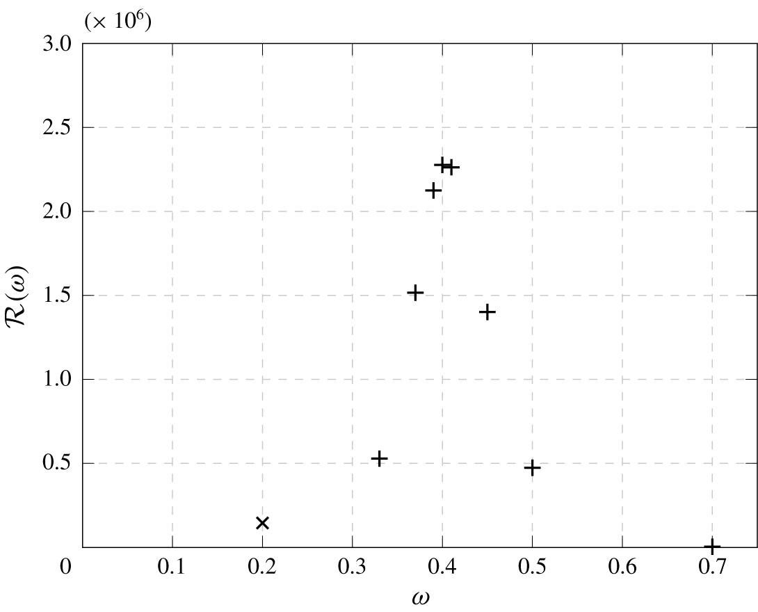
Figure 22.

Resolvent norm at $R=0.3$: low frequency sinuous mode (cross) and higher frequencies varicose modes (pluses).

6 Conclusion and discussion

We have investigated the stability of a jet in cross-flow using several techniques. One of our main aims was to determine to what extent the presence of the pipe in the simulations, as opposed to a simple Dirichlet boundary condition representing its velocity profile, was influencing the results. Further, we wanted to examine the flow behaviour at low jet velocity ratios. Fully nonlinear simulations were performed in order to locate the stability region of the flow in the parameter space. Those results indicate that, at the relatively low Reynolds numbers investigated, the flow is stable at low jet velocity ratios, and a global instability leading to the formation of hairpin vortices in the wake appears as the velocity ratio is increased between $0.35$ and $0.375$. The jet remains attached to the wall and the wake is dominated by a pair of counter-rotating vortices which significantly modify the boundary layer through the lift-up effect. An eigenvalue analysis shows the existence of a branch of damped convective modes as well as a pair of conjugated eigenvalues responsible for a Hopf bifurcation around the velocity ratio $R\simeq 0.37$. Those results are consistent with recent experiments (Klotz et al. Reference Klotz, Gumowski and Wesfreid2019) around the same parameters. The growth rates of this global instability were confirmed with a wave packet analysis. The structures present in the associated eigenvectors form waves strongly amplified in the downstream direction that are consistent with the generation of hairpin vortices in a nonlinear flow. The structural sensitivity was analysed with the help of adjoint eigenmodes. The most unstable pair of eigenmodes is found to be most sensitive to perturbations in a small region just downstream of the jet exit intersecting with the recirculation area. The structural sensitivity remains high in an elongated region extending far downstream. Since the direct and adjoint eigenvectors have almost completely different supports due to the non-normality of the convection terms of the linearized Navier–Stokes equations, the structural sensitivity is found to be very high. The adjoint eigenmode associated with the global instability itself is larger slightly upstream of the jet and inside the pipe close to the jet exit. The computed spectra appear to be numerically converged when the solver tolerances are set to $10^{-14}$. In particular, the spectra of direct and adjoint operators match very well. On the other hand, with solver tolerances of $10^{-10}$, only the most unstable pair of eigenvalues appears to be approximately converged. This phenomenon is explained by the elevated structural sensitivity. Non-modal analysis is also used in order to find the optimal perturbations leading to maximum energy growth at finite times, as well as the optimal periodic forcing. Maximum transient energy growth of the orders of $10^{6}$ and $10^{9}$ are found for velocity ratios $R=0.3$ and $R=0.35$ respectively, two cases where the flow is found to be linearly stable. The optimal perturbations for long times resemble the adjoint eigenvector associated with the global instability, and the response is a wave packet with a structure similar to that of the direct eigenvector.

Those results indicate that even relatively low amplitudes of free-stream turbulence in experiments could in some situations, through transient growth of the perturbations, result in a regular shedding of hairpin vortices that can be confused with a global instability. This could explain the discrepancies between earlier experimental results by Cambonie & Aider (Reference Cambonie and Aider2014) and the numerical works by Peplinski et al. (Reference Peplinski, Schlatter, Henningson, Theofilis and Soria2015b) regarding the existence of steady states for low jet velocity ratios.

On the other hand, the slightly higher values of critical jet velocity ratio presented here compared to those recently reported by Klotz et al. (Reference Klotz, Gumowski and Wesfreid2019) are better explained by a different velocity profile exiting the pipe. They report a flatter velocity profile with thinner shear layers in the absence of a cross-flow. In their experiments, for each value or $Re_{D}$ a critical velocity ratio $R_{c}$ is found such that the amplitude of the hairpin vortices is proportional to $\sqrt{R-R_{c}}$ for $R>R_{c}$ and close to zero for $R<R_{c}$, as expected for a Hopf bifurcation at $R=R_{c}$. This shows that they are indeed observing a bifurcation as opposed to a transient response forced by free-stream turbulence. Similarly, the higher critical velocity ratio found by Peplinski et al. (Reference Peplinski, Schlatter, Henningson, Theofilis and Soria2015b) is likely due to the different velocity profile, with thicker shear layers and devoid of interaction with the cross-flow. In particular, our analysis shows that the eigenvalues are extremely sensitive to perturbations just downstream of the pipe, where their base flow differs significantly from ours.

Further, since the wavemaker is almost entirely situated outside of the pipe, the simulation of the dynamics inside the pipe does not seem to play an important role; the presence of the pipe in the simulation is critical mainly in order to simulate a realistic flow profile at the pipe exit.

Finally, we show that the wavemaker for the mode responsible for the global instability is very elongated and extends far away in the wake. As a consequence, the determination of the growth rate of the instability requires a very long computational domain. This is not required for studying the optimal transient growth as long as the perturbations involved stay confined within the box.