


Impact statement
This research makes a significant contribution to the field of environmental science and pollution management by demonstrating an innovative approach to treating water contaminated with complex mixtures of pollutants. By focusing on the concurrent adsorption of phenol (PHE) and ciprofloxacin onto modified polyethylene terephthalate microplastics (PET MPs), the study addresses a critical gap in existing pollution treatment methodologies, which often overlook the multifaceted nature of industrial discharges. The impact of this study is manifold. First, it provides a scalable solution for the removal of mixed pollutants from water bodies, thereby contributing to safer drinking water and healthier aquatic ecosystems. The use of readily available PET MPs, including waste materials subjected to simple modifications, aligns with sustainability goals by repurposing plastic waste for environmental cleanup. The development and application of advanced modeling techniques, including artificial neural networks, for predicting adsorption capacities, present a leap forward in the design of efficient water treatment systems. These models offer precise, customizable tools for predicting the behavior of pollutants in water thereby enabling the optimization of treatment processes for a variety of contaminants. Finally, the study’s findings have broad implications, extending beyond the immediate environmental benefits. By improving the quality of water, the research supports public health initiatives and contributes to the sustainability of agricultural practices that rely on clean water. The international relevance of this work is underscored by its potential application in diverse geographic and industrial contexts, making it a vital contribution to global efforts to combat water and plastic pollution.
Introduction
Designing water treatment adsorption systems requires comprehensive knowledge of adsorption equilibrium data across a wide concentration range. These data define the limits of a sorbent’s application and significantly impacts the overall costs of the treatment process.
Single-compound adsorption systems, although often oversimplified, are extensively studied. Batch tests can easily provide adsorption isotherms for these systems, and several valid adsorption models exist (Isiuku and Enyoh, Reference Isiuku and Enyoh2019). In contrast, multicomponent systems, which reflect common real situations, are more complex as they involve mixtures of pollutants in industrial discharges (Enyoh and Isiuku, Reference Enyoh and Isiuku2021). For example, ciprofloxacin (CIP) have been found to occur in water with other chemicals from pharmaceutical and personal care products (Lozano et al., Reference Lozano, Carlos, Abrahan, Jürgen, Claudia and Pabel2022). The modeling analysis of experimental data involving such systems presents difficulties due to the great variety of experimental conditions (mainly in terms of pollutant concentration) that can determine the occurrence of unpredictable competitions for the same adsorption sites of the solid surface, interactions between adsorbed molecules, and consequently, a great variation in the adsorption capacity of the involved analytes.
Multicomponent adsorption isotherm theory is important for understanding and predicting the behavior of adsorption processes in real-world situations. By accurately describing the adsorption of multiple components, multicomponent adsorption isotherm theory allows researchers and engineers to design more efficient and effective adsorption systems. Several models can be used for the accounting of competitive adsorption in multicomponent systems, including thermodynamically inconsistent models such as extended Langmuir (EL) and extended Freundlich (EF) isotherms (Amrutha et al., Reference Amrutha and Girish2023). These models have been applied in multiple studies (Agarwal et al., Reference Agarwal, Balomajumder and Thakur2013; Enyoh and Isiuku, Reference Enyoh and Isiuku2021; Pauletto et al., Reference Pauletto, Lütke, Dotto and Salau2021; Peñafiel and Flores, Reference Peñafiel and Flores2023). In order to assess the simultaneous adsorption of paracetamol and nimesulide using activated carbon, Pauletto et al. (Reference Pauletto, Lütke, Dotto and Salau2021) utilized both the EL and EF isotherms. Peñafiel and Flores (Reference Peñafiel and Flores2023) assessed the multi-solute adsorption tests of antibiotics and nonsteroidal anti-inflammatory medications on sugarcane bagasse, namely CIP, sulfamethoxazole, ibuprofen and diclofenac. The simultaneous adsorption of pentachlorophenols and trichlorophenols in binary component solutions on Canna indica L was investigated by Enyoh and Isiuku (Reference Enyoh and Isiuku2021) using EL and EF isotherms. They discovered that neither model could well describe the adsorption data in the binary system. The models’ insensitivity to the system’s interaction and competitive impacts was given as the cause of this.
Empirical evidence now firmly establishes the efficacy of machine learning (ML) models, particularly the artificial neural network (ANN) model, as a nontraditional yet robust tool for predicting multicomponent adsorption equilibrium data. This capability extends to both ideal and nonideal systems, as demonstrated in studies by Kiraz et al. (Reference Kiraz, Canpolat and Erkan2019) and Belhaj et al. (Reference Belhaj, Elraies, Alnarabiji, Abdul Kareem, Shuhli, Mahmood and Belhaj2021). The versatility of ML models goes beyond conventional applications, encompassing isotherm and kinetics modeling, breakthrough curve analysis and process optimization (Pauletto et al., Reference Pauletto, Lütke, Dotto and Salau2021; Enyoh et al., Reference Enyoh, Wang and Senlin2023a, Reference Enyoh, Ovuoraye, Isiuku and Igwegbe2023b). What sets ML models apart is their capacity to learn directly from experimental data, eschewing the need for predefined assumptions about the physicochemical nature influencing the adsorption system, a limitation in many traditional models (Pauletto et al., Reference Pauletto, Lütke, Dotto and Salau2021). This unique characteristic allows ML models to capture the intricate nonlinear relationships inherent in the complex interplay between the input and output variables of the system (Kiraz et al., Reference Kiraz, Canpolat and Erkan2019; El Hanandeh et al., Reference El Hanandeh, Mahdi and Imtiaz2020). This adaptability and data-driven approach position ML models as powerful tools for comprehensively modeling various facets of adsorption processes.
A noticeable gap exists in the literature regarding the application of ANN in adsorption studies involving MPs as adsorbents for pollutants within multicomponent systems (Astray et al., Reference Astray, Soria-Lopez, Barreiro, Mejuto and Cid-Samamed2023). A singular study (Li et al., Reference Li, Yu and Wang2020) attempted to fill this void by employing three ML models – random forest, support vector machine and ANN – to predict partition coefficients (log Kd) for polyethylene (PE), polystyrene and polypropylene MPs in water. Utilizing quantitative structure–property relationship data, the study concluded that these models, boasting correlation coefficients >0.92, could be instrumental in rapidly estimating the absorption of organic contaminants onto MPs (Li et al., Reference Li, Yu and Wang2020).
To the best of our knowledge, no ML model has been presented to predict the adsorption of organic pollutants such phenol (PHE) and CIP by PE terephthalate (PET) MPs in multicomponent solutions that takes into account the equilibrium and kinetics process conditions. PHE, a prevalent pollutant in industrial effluents from chemical and pharmaceutical industries (Mohd, Reference Mohd2020), holds environmental significance. Similarly, CIP, an emerging synthetic fluoroquinolone antibacterial compound widely used in bacterial infection treatment, is omnipresent in aquatic settings due to its widespread use and discharge into the environment through wastewater discharges (Enyoh and Wang, Reference Enyoh and Wang2022). The purpose of this work was to study the competitive interactions and simultaneous adsorption behavior of PHE and CIP onto differently prepared PET MPs such pristine PET MPs (Pr-PET MPs), modified PET MPs (Mod-PET MPs) and aged PET MPs (Ag-PET MPs) in the binary system. In the present study, various multicomponent thermodynamically inconsistent adsorption models, and the ANN model were used to represent the equilibrium adsorption behavior for the binary system. The nonideality of the system was taken account into ANN as well as accounting for the kinetics and thermodynamic operation conditions.
Methods
Data collection
PET MPs were prepared from PET plastic waste collected from a waste bin. The waste was washed, ground into small particles (500 μm), and then subjected to modification (Mod-PET MPs) and aging (Ag-PET MPs) processes using sulfuric acid and hydrogen peroxide at 60°C (Enyoh and Wang, Reference Enyoh and Wang2022). To obtain the adsorption capacities of the adsorbents, batch experiments were conducted in laboratory scale, the results were published in our earlier works (Enyoh and Wang, Reference Enyoh and Wang2022, Reference Enyoh and Wang2023).
Multicomponent modeling
By expanding the single component isotherms, multicomponent isotherm equations were created for the description of adsorption in multi-solute systems. Our earlier publications provided the information needed to compute the models (Enyoh and Wang, Reference Enyoh and Wang2022, Reference Enyoh and Wang2023). In this article, the following equations were utilized:
EL isotherm
The EL isotherm for multicomponent adsorption assumes uniform and equally available active sites on the adsorbent, noninteracting effects among adsorbates and identical adsorption on these uniform sites with consistent energy levels (Girish, Reference Girish2017). The model can be represented in the form presented in equations (1) and (2) for PHE and CIP, respectively.
 $$ {q}_{e,(PHE)}=\frac{q_{\mathit{\max}, PHE}\;{K}_{L, PHE}\;{C}_{e, PHE}}{1+{K}_{L, PHE}{C}_{e, PHE}+{K}_{L, CIP}{C}_{e, CIP}} $$
 $$ {q}_{e,(CIP)}=\frac{q_{\mathit{\max}, CIP}\;{K}_{L, CIP}\;{C}_{e, CIP}}{1+{K}_{L, CIP}{C}_{e, CIP}+{K}_{L, PHE}{C}_{e, PHE}} $$
where qe(PHE) and qe(CIP) are the equilibrium adsorption capacity for PHE and CIP solute (mg/g), respectively. Ce(PHE) and Ce(CIP) represent the equilibrium concentration of single component of PHE and CIP (mg/L), respectively. KL is the Langmuir constant for component (L/mg), and qmax is the monolayer adsorption capacity for PHE/CIP (mg/g). This analysis is performed for a series of experimental values of qe versus Ce for both PHE and CIP using the SOLVER function in Microsoft Excel, as outlined by Enyoh and Isiuku (Reference Enyoh and Isiuku2021).
EF isotherm
The application of the monocomponent Freundlich equation was extended to binary systems, giving rise to the development of the EF isotherm model. This model proves particularly useful in the context of heterogeneous systems where interactions occur among the adsorbed molecules (Girish, Reference Girish2017). The mathematical representation of the EF isotherm for multicomponent systems is expressed as follows:
 $$ {q}_{e,(PHE)}=\frac{K_{F, PHE}\;{C}_{e, PHE}^{\left(\frac{1}{n_{PHE}}\right)+{x}_{PHE}}}{C_{e, PHE}^{x_{PHE}}+{y}_2\;{C}_{e, CIP}^{z_{PHE}}} $$
 $$ {q}_{e,(CIP)}=\frac{K_{F, CIP}\;{C}_{e, CIP}^{\left(\frac{1}{n_{CIP}}\right)+{x}_{CIP}}}{C_{e, CIP}^{x_{CIP}}+{y}_2\;{C}_{e, PHE}^{z_{CIP}}} $$
The adsorption intensities (n) and Freundlich constants (KF) are determined from individual Freundlich models in experimental studies by Enyoh and Wang (Reference Enyoh and Wang2022) for PHE and in Enyoh and Wang (Reference Enyoh and Wang2023) for CIP. For PHE, KF values of 2.58, 1.06 and 1.42 mg/g (L/mg)−1/n, and n values of 2.09, 1.14 and 1.23 were obtained for Pr-PET MPs, Mod-PET MPs and Ag-PET MPs, respectively. For CIP, KF values of 12.26, 12.92 and 12.32, mg/g (L/mg)−1/n and n values of 0.91, 0.80 and 0.88 were obtained for the same materials. The constants x, y and z are determined through the minimization of errors in a nonlinear regression analysis. This analysis is performed for a series of experimental values of qe versus Ce for both PHE and CIP using the SOLVER function in Microsoft Excel, as outlined by Enyoh and Isiuku (Reference Enyoh and Isiuku2021). This approach allows for the accurate determination of these constants, contributing to a comprehensive understanding of the adsorption behavior of PHE and CIP on Pr-PET MPs, Mod-PET MPs and Ag-PET MPs in binary system.
Computational multicomponent modeling-ANNs
An ANN typically comprises an input layer, multiple hidden layers and an output layer. Within the hidden layer, numerous neurons are present, each governed by a unique activation function. The activation function for each neuron involves specific weights and biases. This is mathematically expressed using a general formula, as outlined in equation (5) (Yettou et al., Reference Yettou, Laidi, El Bey, Hanini, Hentabli, Khaldi and Abderrahim2021; Ghaemi et al., Reference Ghaemi, Karimi and Khoshraftar2023):
 $$ {Y}_j^{\left(k+1\right)}=f\left({\sum}_{\left(i=1\right)}^N{X}_i^k{w}_{ij}^k+{b}_i^k\right) $$
where f is the activation (transfer) function. In this study, the best activation (transfer) functions for the model development was hyperbolic tangent (Tanh) activation function. N number of inputs of the neuron and k is the layer (hidden, output), w is the weighting and b is the bias. The target of the model is the adsorption capacity of the Pr-PET MPs, Mod-PET MPs and Ag PET-MPs (in mg/g) for both PHE and CIP in binary system.
In our case, there are 12 inputs to the model, which included data from individual batch studies for PHE and CIP. The input data include; equilibrium concentration (Ce [PHE] and Ce [CIP] in mg/L), initial concentration (in mg/L), pH of the solution, the contact time (t(PHE) and t(CIP) in hours), pseudo-first and second-order kinetic rate constants (PFO-K [PHE] and PFO-K [CIP] in hr−1; PSO-K [PHE] and PSO-K [CIP] in g/mg/hr) and intraparticle diffusion constants (Kid [PHE] and Kid [CIP] in mg/g h1/2). Therefore, in equation (5), X = [Ce(PHE), Ce(CIP), t(PHE), t (CIP), Initial conc., PFO-K (PHE), PFO-K (CIP), PSO-K (PHE), PSO-K (CIP), Kid (PHE), Kid (CIP), pH] and Y = equilibrium adsorption capacities (qe(PHE), qe(CIP)).
In this investigation, the JMP Pro neural networks tool, offering a diverse range of architectures for feedforward backpropagation network implementation, was used. The Broyden–Fletcher–Goldfarb–Shanno (BFGS) algorithm, integrated into JMP Pro (Gotwalt, Reference Gotwalt2010), was used for solving unconstrained nonlinear optimization problems. Despite its slower nature, the BFGS algorithm proved to be a more fitting choice for smaller datasets, exhibiting superior predictive capabilities and enhanced resilience to outliers (Cuiping et al., Reference Cuiping, Zhang and Xiao2022). The number of neurons per layer and the number of layers were adequately adjusted by experimentation to eliminate model architectures that displayed overfitting. The ANN model was built with the following layers: Pr-PET MPs and Ag-PET MPs, the most effective configuration involved a single hidden layer with three neurons each. In contrast, the model tailored for Mod-PET MPs involved two hidden layers, with the first layer boasted five neurons while the second layer, accommodated three neurons. Several precautionary measures were implemented to prevent overfitting of the data. First, data underwent scaling to ensure a harmonized scale, thereby enhancing model predictivity and mitigating biases stemming from scale effects. Second, a monitoring of training and validation losses/accuracy was undertaken, leveraging k-fold cross-validation to detect and avoid overfitting tendencies. These steps fortified the robustness of the model against overfitting, ensuring its reliability and generalizability (Enyoh et al., Reference Enyoh, Duru, Prosper and Wang2023c;Enyoh et al., Reference Enyoh, Ovuoraye, Rabin, Qingyue and Tahir2024).
Interaction effect modeling
In a solution containing multiple pollutants, different types of interactions happen between the adsorbate molecules. The assessment of these interactions can be effectively conducted through the utilization of metrics such as the P-factor and selectivity ratio ( $ {S}_R $
).
$ {S}_R $
).
P-factor
McKay and Al Duri (Reference McKay and Al Duri1987) created the P-factor model, a correlative approach used to compare the binary isotherm data with the monocomponent isotherm data. The P-factor (𝑃𝑓𝑖) clarifies the mechanism by which other components in a binary mixture prevent a component from adhering. It is said as follows:
 $$ {p}_{fi}=\frac{Q_{PHE/ CIP,s}}{Q_{PHE/ CIP,b}} $$
where $ {Q}_{PHE/ CIP,s} $
and
$ {Q}_{PHE/ CIP,s} $
and $ {Q}_{PHE/ CIP,b} $
represent the sorbent monolayer adsorption capacity for the PHE or CIP in the single component solution and the binary system.
$ {Q}_{PHE/ CIP,b} $
represent the sorbent monolayer adsorption capacity for the PHE or CIP in the single component solution and the binary system.
Selectivity ratio
The selectivity ratio (SR) serves as a quantitative measure reflecting the affinity of an adsorbent for a specific component within a binary system. Grounded in the analysis of the adsorbent’s morphology, surface structure and pore distribution, the selectivity ratio delves into the adsorbent’s inclination or preference for one solute in the presence of another (Krishna and van Baten, Reference Krishna and van Baten2020). The selectivity ratio is defined as
 $$ {S}_R=\frac{Q_{PHE,b}}{Q_{CIP,b}} OR\;\frac{Q_{CIP,b}}{Q_{PHE,b}} $$
where $ {Q}_{PHE,b}\; or\;{Q}_{CIP,b} $
represent the adsorption capacity of either PHE or CIP in the binary solution. The value of S
R being less than one implies that the adsorbent has more affinity toward the second component (denominator in equation 7) than the first component (numerator in equation 7).
$ {Q}_{PHE,b}\; or\;{Q}_{CIP,b} $
represent the adsorption capacity of either PHE or CIP in the binary solution. The value of S
R being less than one implies that the adsorbent has more affinity toward the second component (denominator in equation 7) than the first component (numerator in equation 7).
Model evaluation metrics
In order to verify and assess how well the models predict the adsorption equilibrium capacities, statistical metrics like the R 2 (coefficient of determination), mean square error (MSE), root MSE (RMSE) and average absolute error (AAE) given in equations were utilized to analyze and compare the predictive capacities of the models.
 $$ {R}^2=1-\frac{\sum {\left({y}_i-{y}_i^{\ast}\right)}^2}{\sum {\left({y}_i-{{\overline{y}}_i}^{\ast}\right)}^2} $$
 $$ MSE=\frac{1}{\mathrm{N}}\sum_{i=1}^n{\left|{y}_i-{y}_i^{\ast}\right|}^2 $$
 $$ RMSE=\sqrt{\frac{1}{\mathrm{N}}\sum_{i=1}^N{\left({y}_i-{y}_i^{\ast}\right)}^2} $$
 $$ AAE=\frac{1}{\mathrm{N}}\sum_{i=1}^n\mid {y}_i-{y}_i^{\ast}\mid $$
where y
i
is the predicted adsorption capacities qe (mg/g) of PHE and CIP in binary pollution system value by the model, and n is the number of data; $ {y}_i^{\ast } $
is the actual/experimental adsorption capacities qe (mg/g) value and
$ {y}_i^{\ast } $
is the actual/experimental adsorption capacities qe (mg/g) value and $ {{\overline{y}}_i}^{\ast } $
is the average actual/experimental adsorption capacities qe (mg/g). To produce the best ML model, the objective should be to attain the lowest error with RMSE, AAE and the highest with R
2 correlations.
$ {{\overline{y}}_i}^{\ast } $
is the average actual/experimental adsorption capacities qe (mg/g). To produce the best ML model, the objective should be to attain the lowest error with RMSE, AAE and the highest with R
2 correlations.
Results and discussion
Multicomponent modeling
The plots comparing the experimental, EL and EF equilibrium adsorption capacity of PHE and CIP in binary system is presented in Figure 1. The results summary is presented in Table 1.

Figure 1. Comparison of experimental and multicomponent model (extended Langmuir and Freundlich) values for the individual compounds in the binary system (a, c, e) PHE in binary system with CIP for Pr-PET MPs, Mod-PET MPs and Ag-PET MPs, respectively (b, d, f) CIP in binary system with PHE for Pr-PET MPs, Mod-PET MPs and Ag-PET MPs, respectively. Contact time, temperature, shaking speed and pH were set to 60 min, 25°C, 100 rpm and 6, respectively.
Table 1. Parameters of extended Langmuir and Freundlich models for the Pr-PET MPs, Mod-PET MPs and Ag-PET MPs-driven binary adsorption of PHE and CIP

EL isotherm for PET MPs-driven PHE and CIP adsorption in binary system
The EL model, designed as a predictive tool, assumes homogeneity in surface energy and negligible interaction between PHE and CIP. Moreover, it posits that all adsorption sites are equally accessible to both pollutants. Figure 1 illustrates a comparison between EL isotherm predictions and experimental equilibrium data. Critically, the relative scatter diagrams reveal significant fits for Pr-PET and Mod-PET MPs in the binary pollutant system, yielding R² values ranging from 0.7998 to 0.9727. In contrast, Ag-PET MPs exhibit moderate fitting with R² values of 0.5216 for CIP and 0.5508 for PHE, respectively (see Table 1). Pr-PET and Mod-PET MPs show robust fits, suggesting that the EL model is well-suited for predicting the adsorption behavior of PHE and CIP on these surfaces. On the other hand, the moderate fits for Ag-PET MPs indicate that the assumptions of the EL model may not fully capture the interactions at higher equilibrium concentrations occurring in this specific case.
Examining the monolayer adsorption capacities (qmax) for different PET MPs in the binary pollutant system, we find significant values for all adsorbents. Pr-PET MPs demonstrated capacities of 342.10 mg/g for PHE and 2518.23 mg/g for CIP. Mod-PET MPs exhibit even higher capacities with 2970.34 mg/g for PHE and 11927.54 mg/g for CIP. Remarkably, Ag-PET MPs display the highest monolayer adsorption capacities with 3715.73 mg/g for PHE and 14498.79 mg/g for CIP. The order of monolayer adsorption capacity follows Ag-PET MPs > Mod-PET MPs > Pr-PET MPs. The higher capacity recorded for Ag-PET MPs could be due to their favorable surface properties such as its surface area and morphology. However, comparing these results with single-component capacities reported by Enyoh and Wang (Reference Enyoh and Wang2022, Reference Enyoh and Wang2023), a significant enhancement in adsorbent capacity in the binary system of PHE and CIP is evident. These suggest that the interaction between PHE and CIP in the binary system led to synergistic effects, where the presence of one compound enhances the adsorption of the other (Chen et al., Reference Chen, Shi, Wan, Zhao, He and Liu2022; Ke et al., Reference Ke, Zhu, Si, Zhang, Wang and Zhang2023). This synergy is not evident in single-component systems.
EF isotherm for PET MPs-driven PHE and CIP adsorption in binary system
Within the binary pollutant system comprising PHE and CIP, the distinct adsorption capacities for various adsorbents – Pr-PET, Mod-PET and Ag-PET – were determined using the following equations (12-14).
For Pr-PET MPs:
 $$ {q}_{e,(PHE)}=\frac{2.58\;{C}_{e, PHE}^{\left(\frac{1}{2.09}\right)+{x}_{PHE}}}{C_{e, PHE}^{x_{PHE}}+{y}_1{C}_{e, CIP}^{z_{PHE}}} $$
 $$ {q}_{e,(CIP)}=\frac{12.26\;{C}_{e, CIP}^{\left(\frac{1}{0.91}\right)+{x}_{CIP}}}{C_{e, CIP}^{x_{CIP}}+{y}_2{C}_{e, PHE}^{z_{CIP}}} $$
For Mod-PET MPs:
 $$ {q}_{e,(PHE)}=\frac{1.06\;{C}_{e, PHE}^{\left(\frac{1}{1.14}\right)+{x}_{PHE}}}{C_{e, PHE}^{x_{PHE}}+{y}_1{C}_{e, CIP}^{z_{PHE}}} $$
 $$ {q}_{e,(CIP)}=\frac{12.92\;{C}_{e, CIP}^{\left(\frac{1}{0.80}\right)+{x}_{CIP}}}{C_{e, CIP}^{x_{CIP}}+{y}_2{C}_{e, PHE}^{z_{CIP}}} $$
For Ag-PET MPs:
 $$ {q}_{e,(PHE)}=\frac{1.42\;{C}_{e, PHE}^{\left(\frac{1}{1.23}\right)+{x}_{PHE}}}{C_{e, PHE}^{x_{PHE}}+{y}_1{C}_{e, CIP}^{z_{PHE}}} $$
 $$ {q}_{e,(CIP)}=\frac{12.32\;{C}_{e, CIP}^{\left(\frac{1}{0.88}\right)+{x}_{CIP}}}{C_{e, CIP}^{x_{CIP}}+{y}_2{C}_{e, PHE}^{z_{CIP}}} $$
The application of the EF isotherm model proves valuable for heterogeneous systems characterized by interactions among the adsorbed molecules. In Figure 1, a comparison between experimental sorption capacity and predicted values using the EF model for a binary system is presented. The isotherm data indicates the EF model’s suitability in describing the adsorption of PHE and CIP onto Pr-PET MPs and Mod-PET MPs, with R2 values ranging from 0.8283 to 0.9704. The robust performance of the EF model suggests its applicability in capturing the complex interactions and heterogeneity present in the adsorption process on these specific microplastic types. However, the Ag-PET MPs exhibit a lower R2 for PHE (0.3488) and a moderate R2 for CIP (0.5216) in the binary system, as summarized in Table 1. This discrepancy may hint at unique characteristics or complexities in the adsorption process onto Ag-PET MPs that are not fully captured by the EF model.
Computational multicomponent modeling for PET MPs-driven PHE and CIP adsorption in binary system
All the input parameters in the model are considered independent variables. This means that changes in one parameter are not assumed to be directly caused by changes in any other parameter. Each variable is treated as a distinct factor that can influence the output separately. In Table 2, the correlation between different input parameters and the output variable is examined. The strength of correlation is measured using the correlation coefficient (r). The correlation reveal that the strongest correlation exists between the initial concentration (r = 1.00) and qe followed by contact time (r = 0.99) then pH (r = 0.95-0.97). The pseudo-second-order rate constant, although moderately correlated with qe, is the only parameter that is negatively correlated with qe. The correlation analysis provides insights into the relationships between input parameters and output variables. Strong positive correlations suggest direct relationships, while negative correlations indicate an inverse relationship. These findings are crucial for understanding how changes in each parameter may impact the adsorption process and the resulting equilibrium adsorption capacity.
Table 2. Correlation coefficients between the different input parameters and the output for Pr-PET MPs, Mod-PET MPs and Ag-PET MPs

To construct an ANN models with multiple components, an experimental dataset was procured through batch experiments focusing on the adsorption of PHE (Enyoh and Wang, Reference Enyoh and Wang2022) and CIP (Enyoh and Wang, Reference Enyoh and Wang2023). This dataset encapsulated diverse permutations of initial concentrations, contact times, equilibrium concentrations, kinetic parameters and pH levels. The objective was to capture the interactions within a binary system involving PHE and CIP. Following dataset acquisition, a crucial preprocessing step involved the division of the data into a training set and a validation/test set. Initially, 10% of the data were randomly selected and set aside. This reserved subset would later serve as a litmus test for the model’s generalizability, enabling an assessment of its performance on unseen data. The efficacy of the developed ANN models was quantified using various metrics, including R-squared values, RMSE and AAE. These metrics were employed to elucidate the extent to which the models accurately represented the adsorption capacities of PHE and CIP in the binary system across the Pr-PET MPs, Mod-PET MPs and Ag-PET MPs adsorbents. This systematic approach to constructing and evaluating multicomponent ANN models facilitated a robust analysis of the adsorption behaviors of PHE and CIP in a binary system, providing information on the suitability and accuracy of the models across various types of PET MPs adsorbent.
Optimal outcomes were achieved through the implementation of the hyperbolic tangent activation function (TanH). Specifically, for Pr-PET MPs and Ag-PET MPs, the most effective configuration involved a single hidden layer (H1) housing three neurons each (H1_1, H1_2 and H1_3). In contrast, the model tailored for Mod-PET MPs demonstrated superior performance when equipped with two hidden layers. The first layer boasted five neurons (H1_1_1, H1_2_1… H1_5_1), while the second layer, a pivotal component of the enhanced architecture, accommodated three neurons (H2_1_1, H2_2_1 and H2_3_1) (refer to Figure 2). Distinguishingly, each hidden layer carried distinct parameter estimates instrumental in accurately predicting the desired output. The estimates for the different hidden layers are presented in equations (18-31). The numbers preceding each variable are coefficients that determine the weight of each feature in the model, while the ‘n’ subscript indicates various values of each variable. The entire expression is then passed through the TanH function to obtain the final output. This approach allowed for a fine-tuned adaptation to the specific characteristics of Pr-PET MPs, Ag-PET MPs and Mod-PET MPs, showcasing the versatility of the hyperbolic tangent activation function in tailoring the ANN architecture for optimum results.

Figure 2. The multicomponent ANN architecture and plot of ANN predicted qe against actual (experimental) qe for both phenol (PHE) and ciprofloxacin (CIP).
For Pr-PET MPs:
 $$ \mathrm{H}1\_1={\displaystyle \begin{array}{l}\mathrm{TanH}\Big(2.85-0.19\hskip0.3em \ast \hskip0.3em {\left[\mathrm{Ce}\left(\mathrm{CIP}\right)\right]}_{\mathrm{n}}\\ {}-\hskip2px 0.002\hskip0.3em \ast \hskip0.3em {\left[\mathrm{Ce}\left(\mathrm{PHE}\right)\right]}_{\mathrm{n}}-0.02\hskip0.3em \ast \hskip0.3em {[\mathrm{Initial}\ \mathrm{conc}.\ ]}_{\mathrm{n}}\\ {}-\hskip2px 0.15\hskip0.3em \ast \hskip0.3em {\left[\mathrm{Kid}\left(\mathrm{CIP}\right)\right]}_{\mathrm{n}}+98.49\hskip0.3em \ast \hskip0.3em {\left[\mathrm{Kid}\left(\mathrm{PHE}\right)\right]}_{\mathrm{n}}\\ {}-\hskip2px 0.12\hskip0.3em \ast \hskip0.3em {\left[\mathrm{PFO}\hbox{-} \mathrm{K}\left(\mathrm{CIP}\right)\right]}_{\mathrm{n}}-549.94\hskip0.3em \ast \hskip0.3em {\left[\mathrm{PFO}\hbox{-} \mathrm{K}\left(\mathrm{PHE}\right)\right]}_{\mathrm{n}}\\ {}+\hskip2px 0.07\hskip0.3em \ast \hskip0.3em {\left[\mathrm{pH}\right]}_{\mathrm{n}}+0.003\hskip0.3em \ast \hskip0.3em {\left[\mathrm{PSO}\hbox{-} \mathrm{K}\left(\mathrm{CIP}\right)\right]}_{\mathrm{n}}\\ {}-\hskip2px 501.36\hskip0.3em \ast \hskip0.3em {\left[\mathrm{PSO}\hbox{-} \mathrm{K}\left(\mathrm{PHE}\right)\right]}_{\mathrm{n}}\\ {}-0.01\hskip0.3em \ast \hskip0.3em {\left[\mathrm{t}\left(\mathrm{CIP}\right)\right]}_{\mathrm{n}}-\hskip2px 1.02\hskip0.3em \ast \hskip0.3em {\left[\mathrm{t}\left(\mathrm{PHE}\right)\right]}_{\mathrm{n}}\Big)\end{array}} $$
 $$ \mathrm{H}1\_2={\displaystyle \begin{array}{l}\mathrm{TanH}\Big(4.69-0.27\hskip0.3em \ast \hskip0.3em {\left[\mathrm{Ce}\left(\mathrm{CIP}\right)\right]}_{\mathrm{n}}-0.87\hskip0.3em \ast \hskip0.3em {\left[\mathrm{Ce}\left(\mathrm{PHE}\right)\right]}_{\mathrm{n}}\\ {}+\hskip2px 0.01\hskip0.3em \ast \hskip0.3em {[\mathrm{Initial}\ \mathrm{conc}.\ ]}_{\mathrm{n}}+0.26\hskip0.3em \ast \hskip0.3em {\left[\mathrm{Kid}\left(\mathrm{CIP}\right)\right]}_{\mathrm{n}}\\ {}+\hskip2px 34.76\hskip0.3em \ast \hskip0.3em {\left[\mathrm{Kid}\left(\mathrm{PHE}\right)\right]}_{\mathrm{n}}-0.004\hskip0.3em \ast \hskip0.3em {\left[\mathrm{PFO}\hbox{-} \mathrm{K}\left(\mathrm{CIP}\right)\right]}_{\mathrm{n}}\\ {}+\hskip2px 1055.78\hskip0.3em \ast \hskip0.3em {\left[\mathrm{PFO}\hbox{-} \mathrm{K}\left(\mathrm{PHE}\right)\right]}_{\mathrm{n}}-0.17\hskip0.3em \ast \hskip0.3em {\left[\mathrm{pH}\right]}_{\mathrm{n}}\\ {}+\hskip2px 0.36\hskip0.3em \ast \hskip0.3em {\left[\mathrm{PSO}\hbox{-} \mathrm{K}\left(\mathrm{CIP}\right)\right]}_{\mathrm{n}}-699.64\hskip0.3em \ast \hskip0.3em {\left[\mathrm{PSO}\hbox{-} \mathrm{K}\left(\mathrm{PHE}\right)\right]}_{\mathrm{n}}\\ {}-\hskip2px 0.01\hskip0.3em \ast \hskip0.3em {\left[\mathrm{t}\left(\mathrm{CIP}\right)\right]}_{\mathrm{n}}+0.07\hskip0.3em \ast \hskip0.3em {\left[\mathrm{t}\left(\mathrm{PHE}\right)\right]}_{\mathrm{n}}\Big)\end{array}} $$
 $$ \mathrm{H}1\_3={\displaystyle \begin{array}{l}\mathrm{TanH}\Big(0.12-0.04\hskip0.3em \ast \hskip0.3em {\left[\mathrm{Ce}\left(\mathrm{CIP}\right)\right]}_{\mathrm{n}}+0.20\hskip0.3em \ast \hskip0.3em {\left[\mathrm{Ce}\left(\mathrm{PHE}\right)\right]}_{\mathrm{n}}\\ {}+\hskip2px 0.025\hskip0.3em \ast \hskip0.3em {[\mathrm{Initial}\ \mathrm{conc}.\ ]}_{\mathrm{n}}-0.85\hskip0.3em \ast \hskip0.3em {\left[\mathrm{Kid}\left(\mathrm{CIP}\right)\right]}_{\mathrm{n}}\\ {}-\hskip2px 158.64\hskip0.3em \ast \hskip0.3em {\left[\mathrm{Kid}\left(\mathrm{PHE}\right)\right]}_{\mathrm{n}}-0.52\hskip0.3em \ast \hskip0.3em {\left[\mathrm{PFO}\hbox{-} \mathrm{K}\left(\mathrm{CIP}\right)\right]}_{\mathrm{n}}\\ {}-\hskip2px 458.00{\left[\mathrm{PFO}\hbox{-} \mathrm{K}\left(\mathrm{PHE}\right)\right]}_{\mathrm{n}}+0.07\hskip0.3em \ast \hskip0.3em {\left[\mathrm{pH}\right]}_{\mathrm{n}}+0.59\\ {}\hskip0.3em \ast \hskip0.3em \Big[\mathrm{PSO}{\hbox{-} \mathrm{K}\left(\mathrm{CIP}\right)\Big]}_{\mathrm{n}}-698.33\hskip0.3em \ast \hskip0.3em {\left[\mathrm{PSO}\hbox{-} \mathrm{K}\left(\mathrm{PHE}\right)\right]}_{\mathrm{n}}\\ {}-\hskip2px 0.03\hskip0.3em \ast \hskip0.3em {\left[\mathrm{t}\left(\mathrm{CIP}\right)\right]}_{\mathrm{n}}+1.30{\left[\mathrm{t}\left(\mathrm{PHE}\right)\right]}_{\mathrm{n}}\Big)\end{array}} $$
For Mod-PET MPs:
 $$ \mathrm{H}2\_1\_1={\displaystyle \begin{array}{l}\mathrm{TanH}\Big(-1315306875291720-0.01\hskip0.3em \ast \hskip0.3em {\left[\mathrm{Ce}\left(\mathrm{CIP}\right)\right]}_{\mathrm{n}}\\ {}-\hskip2px 0.08\hskip0.3em \ast \hskip0.3em {\left[\mathrm{Ce}\left(\mathrm{PHE}\right)\right]}_{\mathrm{n}}-0.01\ast {[\mathrm{Initial}\ \mathrm{conc}.\ ]}_{\mathrm{n}}\\ {}-\hskip2px 0.004\hskip0.3em \ast \hskip0.3em {\left[\mathrm{Kid}\left(\mathrm{CIP}\right)\right]}_{\mathrm{n}}-71.86\hskip0.3em \ast \hskip0.3em {\left[\mathrm{Kid}\left(\mathrm{PHE}\right)\right]}_{\mathrm{n}}\\ {}+\hskip2px 0.002\hskip0.3em \ast \hskip0.3em {\left[\mathrm{PFO}\hbox{-} \mathrm{K}\left(\mathrm{CIP}\right)\right]}_{\mathrm{n}}+266.13\\ {}\hskip0.3em \ast \hskip0.3em \Big[\mathrm{PFO}{\hbox{-} \mathrm{K}\left(\mathrm{PHE}\right)\Big]}_{\mathrm{n}}-0.03\hskip0.3em \ast \hskip0.3em {\left[\mathrm{pH}\right]}_{\mathrm{n}}\\ {}+714840693093327\hskip0.3em \ast \hskip0.3em {\left[\mathrm{PSO}\hbox{-} \mathrm{K}\left(\mathrm{CIP}\right)\right]}_{\mathrm{n}}\\ {}+\hskip2px 43.09\hskip0.3em \ast \hskip0.3em {\left[\mathrm{PSO}\hbox{-} \mathrm{K}\left(\mathrm{PHE}\right)\right]}_{\mathrm{n}}-0.02\hskip0.3em \ast \hskip0.3em {\left[\mathrm{t}\left(\mathrm{CIP}\right)\right]}_{\mathrm{n}}\\ {}-\hskip2px 0.27\hskip0.3em \ast \hskip0.3em {\left[\mathrm{t}\left(\mathrm{PHE}\right)\right]}_{\mathrm{n}}\Big)\end{array}} $$
 $$ \mathrm{H}2\_2\_1={\displaystyle \begin{array}{l}\mathrm{TanH}\Big(-1001299057845485+0.02\hskip0.3em \ast \hskip0.3em {\left[\mathrm{Ce}\left(\mathrm{CIP}\right)\right]}_{\mathrm{n}}\\ {}+\hskip2px 0.05\hskip0.3em \ast \hskip0.3em {\left[\mathrm{Ce}\left(\mathrm{PHE}\right)\right]}_{\mathrm{n}}+0.006\hskip0.3em \ast \hskip0.3em {[\mathrm{Initial}\ \mathrm{conc}.\ ]}_{\mathrm{n}}\\ {}-\hskip2px 0.003\hskip0.3em \ast \hskip0.3em {\left[\mathrm{Kid}\left(\mathrm{CIP}\right)\right]}_{\mathrm{n}}+43.74\hskip0.3em \ast \hskip0.3em {\left[\mathrm{Kid}\left(\mathrm{PHE}\right)\right]}_{\mathrm{n}}\\ {}+\hskip2px 0.0002\hskip0.3em \ast \hskip0.3em {\left[\mathrm{PFO}\hbox{-} \mathrm{K}\left(\mathrm{CIP}\right)\right]}_{\mathrm{n}}-227.34\\ {}\hskip0.3em \ast \hskip0.3em \Big[\mathrm{PFO}{\hbox{-} \mathrm{K}\left(\mathrm{PHE}\right)\Big]}_{\mathrm{n}}+0.019\hskip0.3em \ast \hskip0.3em {\left[\mathrm{pH}\right]}_{\mathrm{n}}\\ {}+544184270568198\hskip0.3em \ast \hskip0.3em {\left[\mathrm{PSO}\hbox{-} \mathrm{K}\left(\mathrm{CIP}\right)\right]}_{\mathrm{n}}\\ {}+\hskip2px 13.59\hskip0.3em \ast \hskip0.3em {\left[\mathrm{PSO}\hbox{-} \mathrm{K}\left(\mathrm{PHE}\right)\right]}_{\mathrm{n}}+0.014\hskip0.3em \ast \hskip0.3em {\left[\mathrm{t}\left(\mathrm{CIP}\right)\right]}_{\mathrm{n}}\\ {}+\hskip2px 0.17\hskip0.3em \ast \hskip0.3em {\left[\mathrm{t}\left(\mathrm{PHE}\right)\right]}_{\mathrm{n}}\Big)\end{array}} $$
 $$ \mathrm{H}2\_3\_1={\displaystyle \begin{array}{l}\mathrm{TanH}\Big(-186587478237282+0.09\hskip0.3em \ast \hskip0.3em {\left[\mathrm{Ce}\left(\mathrm{CIP}\right)\right]}_{\mathrm{n}}\\ {}-\hskip2px 0.05\hskip0.3em \ast \hskip0.3em {\left[\mathrm{Ce}\left(\mathrm{PHE}\right)\right]}_{\mathrm{n}}-0.01\hskip0.3em \ast \hskip0.3em {[\mathrm{Initial}\ \mathrm{conc}.\ ]}_{\mathrm{n}}\\ {}+\hskip2px 0.0004\hskip0.3em \ast \hskip0.3em {\left[\mathrm{Kid}\left(\mathrm{CIP}\right)\right]}_{\mathrm{n}}-94.69\hskip0.3em \ast \hskip0.3em {\left[\mathrm{Kid}\left(\mathrm{PHE}\right)\right]}_{\mathrm{n}}\\ {}-\hskip2px 0.001\hskip0.3em \ast \hskip0.3em {\left[\mathrm{PFO}\hbox{-} \mathrm{K}\left(\mathrm{CIP}\right)\right]}_{\mathrm{n}}-182.65\\ {}\hskip0.3em \ast \hskip0.3em \Big[\mathrm{PFO}{\hbox{-} \hskip2px \mathrm{K}\left(\mathrm{PHE}\right)\Big]}_{\mathrm{n}}+0.006\hskip0.3em \ast \hskip0.3em {\left[\mathrm{pH}\right]}_{\mathrm{n}}\\ {}+\hskip2px 101406238172436\hskip0.3em \ast \hskip0.3em {\left[\mathrm{PSO}\hbox{-} \mathrm{K}\left(\mathrm{CIP}\right)\right]}_{\mathrm{n}}\\ {}-\hskip2px 61.10\hskip0.3em \ast \hskip0.3em {\left[\mathrm{PSO}\hbox{-} \mathrm{K}\left(\mathrm{PHE}\right)\right]}_{\mathrm{n}}-0.02\hskip0.3em \ast \hskip0.3em {\left[\mathrm{t}\left(\mathrm{CIP}\right)\right]}_{\mathrm{n}}\\ {}-\hskip2px 0.19\hskip0.3em \ast \hskip0.3em {\left[\mathrm{t}\left(\mathrm{PHE}\right)\right]}_{\mathrm{n}}\Big)\end{array}} $$
 $$ \mathrm{H}1\_1\_1={\displaystyle \begin{array}{l}\mathrm{TanH}\Big(-0.09-0.27\hskip0.3em \ast \hskip0.3em \left[\mathrm{H}2\_1\_1\right]\\ {}-\hskip2px 0.62\hskip0.3em \ast \hskip0.3em \left[\mathrm{H}2\_2\_1\right]+0.34\hskip0.3em \ast \hskip0.3em \left[\mathrm{H}2\_3\_1\right]\Big)\end{array}} $$
 $$ \mathrm{H}1\_2\_1={\displaystyle \begin{array}{l}\mathrm{TanH}\Big(-0.2-0.05\hskip0.3em \ast \hskip0.3em \left[\mathrm{H}2\_1\_1\right]+0.18\hskip0.3em \ast \hskip0.3em \left[\mathrm{H}2\_2\_1\right]\\ {}+\hskip2px 0.18\hskip0.3em \ast \hskip0.3em \left[\mathrm{H}2\_3\_1\right]\Big)\end{array}} $$
 $$ \mathrm{H}1\_3\_1={\displaystyle \begin{array}{l}\mathrm{TanH}\Big(-0.07-0.42\hskip0.3em \ast \hskip0.3em \left[\mathrm{H}2\_1\_1\right]\\ {}+\hskip2px 0.18\hskip0.3em \ast \hskip0.3em \left[\mathrm{H}2\_2\_1\right]+0.01\hskip0.3em \ast \hskip0.3em \left[\mathrm{H}2\_3\_1\right]\Big)\end{array}} $$
 $$ \mathrm{H}1\_4\_1={\displaystyle \begin{array}{l}\mathrm{TanH}\Big(0.25+0.22\hskip0.3em \ast \hskip0.3em \left[\mathrm{H}2\_1\_1\right]-0.31\hskip0.3em \ast \hskip0.3em \left[\mathrm{H}2\_2\_1\right]\\ {}+\hskip2px 0.02\hskip0.3em \ast \hskip0.3em \left[\mathrm{H}2\_3\_1\right]\Big)\end{array}} $$
 $$ \mathrm{H}1\_5\_1={\displaystyle \begin{array}{l}\mathrm{TanH}\Big(0.10+0.38\hskip0.3em \ast \hskip0.3em \left[\mathrm{H}2\_1\_1\right]+0.02\hskip0.3em \ast \hskip0.3em \left[\mathrm{H}2\_2\_1\right]\\ {}+\hskip2px 0.08\hskip0.3em \ast \hskip0.3em \left[\mathrm{H}2\_3\_1\right]\Big)\end{array}} $$
Ag-PET MPs:
 $$ \hskip-6.5em \mathrm{H}1\_1\_1={\displaystyle \begin{array}{l}\mathrm{TanH}\;\Big(\hbox{-} 8.81+0.56\hskip0.3em \ast \hskip0.3em {\left[\mathrm{Ce}\left(\mathrm{CIP}\right)\right]}_{\mathrm{n}}\;\\ {}\hbox{-} 0.20\hskip0.3em \ast \hskip0.3em {\left[\mathrm{Ce}\left(\mathrm{PHE}\right)\right]}_{\mathrm{n}}\hbox{-} 0.0001\hskip0.3em \ast \hskip0.3em {\left[\mathrm{Initial}\ \mathrm{conc}.\right]}_{\mathrm{n}}\\ {}\hbox{-} 0.01\hskip0.3em \ast \hskip0.3em {\left[\mathrm{Kid}\left(\mathrm{CIP}\right)\right]}_{\mathrm{n}}\hbox{-} 85.40\hskip0.3em \ast \hskip0.3em {\left[\mathrm{Kid}\left(\mathrm{PHE}\right)\right]}_{\mathrm{n}}\\ {}+0.33\hskip0.3em \ast \hskip0.3em {\left[\mathrm{PFO}\hbox{-} \mathrm{K}\left(\mathrm{CIP}\right)\right]}_{\mathrm{n}}\\ {}+8893.82\hskip0.3em \ast \hskip0.3em {\left[\mathrm{PFO}\hbox{-} \mathrm{K}\left(\mathrm{PHE}\right)\right]}_{\mathrm{n}}+0.19\hskip0.3em \ast \hskip0.3em {\left[\mathrm{pH}\right]}_{\mathrm{n}}\;\\ {}+0.56\hskip0.3em \ast \hskip0.3em {\left[\mathrm{PSO}\hbox{-} \mathrm{K}\left(\mathrm{CIP}\right)\right]}_{\mathrm{n}}\\ {}+230.42\hskip0.3em \ast \hskip0.3em {\left[\mathrm{PSO}\hbox{-} \mathrm{K}\left(\mathrm{PHE}\right)\right]}_{\mathrm{n}}\\ {}+\hbox{-} 0.02\hskip0.3em \ast \hskip0.3em {\left[\mathrm{t}\left(\mathrm{CIP}\right)\right]}_{\mathrm{n}}\hbox{-} 0.31\hskip0.3em \ast \hskip0.3em \left[\mathrm{t}\left(\mathrm{PHE}\right)\right]\end{array}} $$
 $$ \mathrm{H}1\_2\_1={\displaystyle \begin{array}{l}\mathrm{TanH}\Big(2.04-0.37\hskip0.3em \ast \hskip0.3em {\left[\mathrm{Ce}\left(\mathrm{CIP}\right)\right]}_{\mathrm{n}}\\ {}-\hskip2px 0.66\hskip0.3em \ast \hskip0.3em {\left[\mathrm{Ce}\left(\mathrm{PHE}\right)\right]}_{\mathrm{n}}+0.03\hskip0.3em \ast \hskip0.3em {[\mathrm{Initial}\ \mathrm{conc}.\ ]}_{\mathrm{n}}\\ {}+\hskip2px 0.24\hskip0.3em \ast \hskip0.3em {\left[\mathrm{Kid}\left(\mathrm{CIP}\right)\right]}_{\mathrm{n}}-131.54\hskip0.3em \ast \hskip0.3em \left[\mathrm{Kid}\left(\mathrm{PHE}\right)\right]\\ {}+\hskip2px 0.78\hskip0.3em \ast \hskip0.3em \left[\mathrm{PFO}\hbox{-} \mathrm{K}\left(\mathrm{CIP}\right)\right]-361.53\hskip0.3em \ast \hskip0.3em {\left[\mathrm{PFO}\hbox{-} \mathrm{K}\left(\mathrm{PHE}\right)\right]}_{\mathrm{n}}\\ {}+\hskip2px 0.05\hskip0.3em \ast \hskip0.3em \left[\mathrm{pH}\right]-0.39\hskip0.3em \ast \hskip0.3em {\left[\mathrm{PSO}\hbox{-} \mathrm{K}\left(\mathrm{CIP}\right)\right]}_{\mathrm{n}}\\ {}+\hskip2px 219.59\hskip0.3em \ast \hskip0.3em {\left[\mathrm{PSO}\hbox{-} \mathrm{K}\left(\mathrm{PHE}\right)\right]}_{\mathrm{n}}+0.02\hskip0.3em \ast \hskip0.3em {\left[\mathrm{t}\left(\mathrm{CIP}\right)\right]}_{\mathrm{n}}\\ {}-\hskip2px 0.89\hskip0.3em \ast \hskip0.3em {\left[\mathrm{t}\left(\mathrm{PHE}\right)\right]}_{\mathrm{n}}\Big)\end{array}} $$
 $$ \mathrm{H}1\_3\_1={\displaystyle \begin{array}{l}\mathrm{TanH}\Big(1.78-0.22\hskip0.3em \ast \hskip0.3em {\left[\mathrm{Ce}\left(\mathrm{CIP}\right)\right]}_{\mathrm{n}}\\ {}+\hskip2px 0.38\hskip0.3em \ast \hskip0.3em {\left[\mathrm{Ce}\left(\mathrm{PHE}\right)\right]}_{\mathrm{n}}-0.06\hskip0.3em \ast \hskip0.3em {[\mathrm{Initial}\ \mathrm{conc}.\ ]}_{\mathrm{n}}\\ {}+\hskip2px 0.56\hskip0.3em \ast \hskip0.3em {\left[\mathrm{Kid}\left(\mathrm{CIP}\right)\right]}_{\mathrm{n}}+18.01\hskip0.3em \ast \hskip0.3em {\left[\mathrm{Kid}\left(\mathrm{PHE}\right)\right]}_{\mathrm{n}}\\ {}-\hskip2px 0.41\hskip0.3em \ast \hskip0.3em {\left[\mathrm{PFO}\hbox{-} \mathrm{K}\left(\mathrm{CIP}\right)\right]}_{\mathrm{n}}-1828.756\hskip0.3em \ast \hskip0.3em {\left[\mathrm{PFO}\hbox{-} \mathrm{K}\left(\mathrm{PHE}\right)\right]}_{\mathrm{n}}\\ {}+\hskip2px 0.02\hskip0.3em \ast \hskip0.3em {\left[\mathrm{pH}\right]}_{\mathrm{n}}-0.14\hskip0.3em \ast \hskip0.3em {\left[\mathrm{PSO}\hbox{-} \mathrm{K}\left(\mathrm{CIP}\right)\right]}_{\mathrm{n}}\\ {}-\hskip2px 249.27\hskip0.3em \ast \hskip0.3em {\left[\mathrm{PSO}\hbox{-} \mathrm{K}\left(\mathrm{PHE}\right)\right]}_{\mathrm{n}}+0.10\hskip0.3em \ast \hskip0.3em {\left[\mathrm{t}\left(\mathrm{CIP}\right)\right]}_{\mathrm{n}}\\ {}-\hskip2px 0.28\hskip0.3em \ast \hskip0.3em {\left[\mathrm{t}\left(\mathrm{PHE}\right)\right]}_{\mathrm{n}}\Big)\end{array}} $$
After fine-tuning the ANN, refined models were established to capture the adsorption capacities of PHE and CIP on PET MPs adsorbents in binary pollutant system (equations 32–37). Subsequently, these updated models were deployed to forecast the adsorption capacities of Pr-PET MPs, Mod-PET MPs and Ag-PET MPs within a binary system for both PHE and CIP (Figure 2). Impressively, these models exhibited commendable performance metrics, showcasing elevated R2 values which ranged from 0.989 to 0.999, alongside low RMSE which ranged from 0.001 to 0.413 and AAE which ranged from 0.009 to 0.327. The R-squared values offered insights into the proportion of variance in the adsorption capacity explained by the models, providing a measure of their goodness of fit (Enyoh et al., Reference Enyoh, Ovuoraye, Rabin, Qingyue and Tahir2024). Simultaneously, RMSE gauged the overall accuracy of the models by quantifying the average magnitude of the prediction errors. Additionally, AAE values provided a metric for the average absolute deviation between predicted and observed values, further contributing to the comprehensive evaluation of model performance (Dobrzański et al., Reference Dobrzański, Trzaska and Dobrzańska-Danikiewicz2014). This robust evaluation underscores the efficacy of the optimized ANN models in accurately predicting the adsorption behaviors of PHE and CIP on various PET MPs in a binary system.
Pr-PET MPs:
 $$ \mathrm{Predicted}\;\mathrm{qe}\left(\mathrm{PHE}\right){\displaystyle \begin{array}{l}=2.898+1.223\ast \left[\mathrm{H}1\_1\right]\\ {}-\hskip2px 3.789\ast \left[\mathrm{H}1\_2\right]-0.243\ast \left[\mathrm{H}1\_3\right];\\ {}{\boldsymbol{R}}^{\boldsymbol{2}}=\boldsymbol{0.9998},\boldsymbol{RMSE}=\boldsymbol{0.0273},\\ {}\boldsymbol{AAE}=\boldsymbol{0.0122}\end{array}} $$
 $$ \mathrm{Predicted}\;\mathrm{qe}\left(\mathrm{CIP}\right){\displaystyle \begin{array}{l}=2.635+1.310\hskip0.3em \ast \hskip0.3em \left[\mathrm{H}1\_1\right]\\ {}-\hskip2px 3.633\hskip0.3em \ast \hskip0.3em \left[\mathrm{H}1\_2\right]-0.278\hskip0.3em \ast \hskip0.3em \left[\mathrm{H}1\_3\right];\\ {}{\boldsymbol{R}}^{\boldsymbol{2}}=\boldsymbol{0.9999},\boldsymbol{RMSE}=\boldsymbol{0.0207},\\ {}\boldsymbol{AAE}=\boldsymbol{0.0093}\end{array}} $$
Mod-PET MPs:
 $$ \mathrm{Predicted}\;\mathrm{qe}\left(\mathrm{PHE}\right){\displaystyle \begin{array}{l}=3.973-3.093\hskip0.3em \ast \hskip0.3em \left[\mathrm{H}1\_1\_1\right]\\ {}+\hskip2px 3.120\hskip0.3em \ast \hskip0.3em \left[\mathrm{H}1\_2\_1\right]+3.408\hskip0.3em \ast \hskip0.3em \left[\mathrm{H}1\_3\_1\right]\\ {}+\hskip2px 1.226\hskip0.3em \ast \hskip0.3em \left[\mathrm{H}1\_4\_1\right]-2.296\hskip0.3em \ast \hskip0.3em \left[\mathrm{H}1\_5\_1\right];\\ {}{\boldsymbol{R}}^{\boldsymbol{2}}=\boldsymbol{0.9638},\boldsymbol{RMSE}=\boldsymbol{0.4125},\\ {}\boldsymbol{AAE}=\boldsymbol{0.3267}\end{array}} $$
 $$ \mathrm{Predicted}\;\mathrm{qe}\left(\mathrm{CIP}\right){\displaystyle \begin{array}{l}=3.681-3.059\hskip0.3em \ast \hskip0.3em \left[\mathrm{H}1\_1\_1\right]\\ {}+\hskip2px 1.400\hskip0.3em \ast \hskip0.3em \left[\mathrm{H}1\_2\_1\right]+2.694\hskip0.3em \ast \hskip0.3em \left[\mathrm{H}1\_3\_1\right]\\ {}-\hskip2px 0.754\hskip0.3em \ast \hskip0.3em \left[\mathrm{H}1\_4\_1\right]-1.095\hskip0.3em \ast \hskip0.3em \left[\mathrm{H}1\_5\_1\right];\\ {}{\boldsymbol{R}}^{\boldsymbol{2}}=\boldsymbol{0.9746},\boldsymbol{RMSE}=\boldsymbol{0.3369},\\ {}\boldsymbol{AAE}=\boldsymbol{0.2732}\end{array}} $$
Ag-PET MPs:
 $$ \mathrm{Predicted}\;\mathrm{qe}\left(\mathrm{PHE}\right){\displaystyle \begin{array}{l}=2.027-3.112\hskip0.3em \ast \hskip0.3em \left[\mathrm{H}1\_1\_1\right]\\ {}-\hskip2px 4.370\hskip0.3em \ast \hskip0.3em \left[\mathrm{H}1\_2\_1\right]-2.895\hskip0.3em \ast \hskip0.3em \left[\mathrm{H}1\_3\_1\right];\\ {}{\boldsymbol{R}}^{\boldsymbol{2}}=\boldsymbol{0.9999},\boldsymbol{RMSE}=\boldsymbol{0.0001},\\ {}\boldsymbol{AAE}=\boldsymbol{0.0002}\end{array}} $$
 $$ \mathrm{Predicted}\;\mathrm{qe}\left(\mathrm{CIP}\right){\displaystyle \begin{array}{l}=1.736-3.232\hskip0.3em \ast \hskip0.3em \left[\mathrm{H}1\_1\_1\right]\\ {}-\hskip2px 4.448\hskip0.3em \ast \hskip0.3em \left[\mathrm{H}1\_2\_1\right]-3.088\hskip0.3em \ast \hskip0.3em \left[\mathrm{H}1\_3\_1\right];\\ {}{\boldsymbol{R}}^{\boldsymbol{2}}=\boldsymbol{0.9999},\boldsymbol{RMSE}=\boldsymbol{0.0071},\\ {}\boldsymbol{AAE}=\boldsymbol{0.0032}\end{array}} $$
Interactive mechanism of PET MPs-driven competitive adsorption of PHE and CIP in binary system
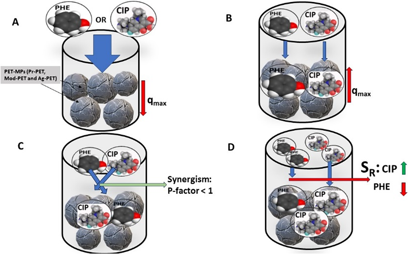
The mechanisms or interactions of pollutants are the most significant phenomena in multicomponent adsorption equilibria. Gaining a deeper understanding of these mechanisms is essential in achieving better results and analyzing any adsorption system. One of the primary considerations for sorbent design is the particle surface charges, which determine the interactions. According to Yang (Reference Yang2003), the dispersion interaction for a sorbate molecule is improved by the surface atom’s polarizability, which increases with the atomic weight of elements. Evaluation of interactive effects can be achieved via computing P-factor and SR (Figure 3). The interaction of the PHE and CIP in the binary adsorption system to the PET MP adsorbents is demonstrated in Figure 4.

Figure 3. Competition constants of PHE and CIP by the PET MPs in a binary system.

Figure 4. The graphical representation of the interactive effect of PHE and CIP in binary adsorption system to PET MPs adsorbent. The single component adsorption driven by the PET MPs had lower monolayer adsorption capacity (qmax) (a) while in binary solution the capacity increased (b). The interaction of the PHE and CIP in the binary solution was synergistic with Pf < 1 (c); however, the PET MPs was more selective to CIP compared to PHE (d).
The P-factor is dimensionless metric, which serves as a concise model describing molecular interactions, employing a ratio of monolayer capacity (q max) for correlation (McKay and Al-Duri, Reference McKay and Al-Duri1987; Chana et al., Reference Chana, Cheung, Allen and McKay2017; Wakkel et al., Reference Wakkel, Besma and Fethi2020). It systematically contrasts equilibrium data involving multiple components. The Pf value, a pivotal parameter in this model, defines the nature of interactions – whether they entail inhibition, enhancement or noninterference – between two components. A Pf value of 1 indicates unimpeded interaction between PHE and CIP in the binary adsorption system by the different PET MPs adsorbents, while Pf>1 signifies that the adsorption of a component (PHE or CIP) is inhibited in the presence of other solutes (PHE or CIP). Conversely, Pf<1 denotes enhanced or synergistic adsorption of PHE or CIP when coexisting.
The Pf obtained for the different pollutants were <1 (Figure 3) and, following the classification of Pf values (< 1), it reveals that both PHE and CIP exhibit enhanced adsorption in the binary system when present together with PET MPs. This finding suggests a synergistic effect or mutual promotion in the adsorption behavior of PHE and CIP when adsorbed by the PET MPs. This is in agreement with the monolayer adsorption capacities predicted by the EL isotherm model. This enhanced adsorption could be attributed to various factors, such as the potential cooperative interactions between PHE and CIP molecules, as well as favorable conditions created by the PET MPs that facilitate the adsorption of both pollutants. However, the PET MPs showed greater affinity toward CIP with lower Pf values compared PHE. This observation may be corroborated by the study of Peñafiel and Flores (Reference Peñafiel and Flores2023), who reported that the presence of CIP did not interfere with the adsorption of other solutes onto sugarcane bagasse in multicomponent system.
Selectivity plays a pivotal role in elucidating the complexities of the adsorption mechanism, offering insights into a component’s ability to discriminate among multiple elements in the same solution (Zhang et al., Reference Zhang, Liu, Zhang, Wang, Xu, Deng, Zeng and Deng2019). This crucial aspect is quantified by the selectivity ratio (SR), which delineates the adsorbent’s preference for a specific component over others, contingent upon its morphology, surface structure and pore distribution (Amrutha et al., Reference Amrutha and Girish2023). In the binary system, the computed SR values for both PHE and CIP are visually represented in Figure 3. Results showed that the SR values for PHE range from 0.136 for Pr-PET MPs to 0.256 for Ag-PET MPs, all falling below 1. Conversely, for CIP, the SR values range from 3.902 for Ag-PET MPs to 7.361 for Pr-PET MPs, all exceeding 1. This disparity suggests that the PET MPs exhibit a higher selectivity toward CIP as compared to PHE. The observed selectivity trend aligns with the corroborating Pf results, reinforcing the notion that PET MPs possess a heightened affinity for CIP over PHE within the binary system. This could be due to molecular interaction, as the PET MPs may possess specific chemical or structural attributes that favor interactions with CIP molecules over PHE. The molecular characteristics of CIP align more favorably with the surface properties of PET MPs in comparison to PHE. In the adsorption process conducted at a pH range of 5-6 (Enyoh and Wang, Reference Enyoh and Wang2022, Reference Enyoh and Wang2023), CIP exhibits a positive charge distribution, existing as cations, while PET MPs carry a negative charge (Enyoh and Wang, Reference Enyoh and Wang2023). This electrostatic compatibility facilitates the easy adsorption of CIP onto PET MPs, resulting in high selectivity. Contrastingly, at the same pH conditions, PHE, which exists as a neutral molecule due to a pH below its pKa of 9.89, lacks the dissociation seen in CIP. Consequently, the hydrogen bonding efficiency of phenolate ions diminishes owing to the electron-rich nature of the hydrogen atom (Enyoh and Wang, Reference Enyoh and Wang2022). As a result, PHE are adsorbed successfully on the PET MPs surface as intact molecules rather than phenolate ions, diminishing the selectivity of PHE by the different PET MPs adsorbents. This difference in interaction mechanisms contributes to the observed variations in selectivity between CIP and PHE on the PET MPs surface. Furthermore, the morphology and pore distribution of PET MPs might be more conducive to accommodating CIP molecules, leading to a higher selectivity. If CIP molecules fit more effectively within the pores or surface features of PET MPs, it could result in enhanced adsorption.
Conclusion
This study has provided information into the complex adsorption dynamics of PHE and CIP onto various PET MPs. Through the utilization of advanced models such as the EL, EF isotherms and a novel ANN model, the research successfully characterized the multicomponent adsorption equilibria, considering both equilibrium and kinetics process conditions. The models demonstrated commendable performance metrics, particularly the ANN model, with low errors and high prediction capacity of 98.9–99 %. The interaction of PHE and CIP adsorption onto PET MPs in the binary system is synergistic. However, the PET MPs adsorbents had higher selectivity toward CIP compared to PHE, revealing distinct preferences in the multicomponent system. While the EL isotherm showed better fitting for specific PET MP types, the EF model proved effective for Pr-PET MPs and Mod-PET MPs but exhibited limitations for Ag-PET MPs. This study contributes to our understanding of multicomponent adsorption onto PET MPs, highlighting the significance of considering various PET MP types and the necessity for tailored models to capture the interactions within these systems. The findings have implications for environmental remediation and underscore the need for further exploration into the adsorption behavior of different MPs types in diverse pollutant scenarios.
Open peer review
To view the open peer review materials for this article, please visit http://doi.org/10.1017/plc.2024.23.
Data availability statement
All data generated or analyzed during this study are included in the article and its supplementary file.
Author contribution
C.E.E.: Conceptualization, methodology, data curation, formal analysis, software, validation and writing-original draft. Q.W.: Supervision, funding acquisition, project administration, writing-reviewing and editing
Financial support
This study was partially supported by the Special Funds for Innovative Area Research (No. 20120015, FY 2008-FY2012) and Basic Research (B) (No. 24310005, FY2012-FY2014; No. 18H03384, FY2017 FY2020; No. 22H03747, FY2022-FY2024) of Grant-in-Aid for Scientific Research of Japanese Ministry of Education, Culture, Sports, Science and Technology (MEXT).
Competing interest
The authors declare none.
Consent to publish
All authors have read and agreed to the published version of the manuscript.


 Open access
Comments
No accompanying comment.