


1. Introduction
Land-fast sea ice, or fast ice, is often attached to the coastline or ice shelves, and provides a stable buffer zone from the mobile pack ice drifting offshore (Hoppmann and others, Reference Hoppmann2015). Fast ice is a navigational obstacle, particularly for ships that need to be docked in the harbors of Antarctic stations. The physical factors affecting the annual cycle of fast ice thickness in Prydz Bay include the incoming and outgoing solar shortwave and thermal longwave radiative fluxes; turbulent surface fluxes of sensible and latent heat; density, thermal conductivity and depth of snow; as well as oceanic heat flux at the ice base (Heil and others, Reference Heil, Allison and Lytle1996; Lei and others, Reference Lei, Li, Cheng, Zhang and Heil2010; Yang and others, Reference Yang2015; Zhao and others, Reference Zhao2019a). Among those factors, the atmospheric forcing plays a dominant role in land-ice mass balance (Heil, Reference Heil2006). The oceanic heat flux is difficult to observe directly, but the shallow bathymetry underneath the fast ice cover limits the magnitude of the oceanic heat flux, making it less important than atmospheric forcing on ice mass balance (Heil, Reference Heil2006; Yang and others, Reference Yang2015). Snow provides an insulating layer for the ice layer below, and reflects most of the incoming shortwave radiation back to space because of a high surface albedo. The surface albedo depends on the snow thickness, grain size and shape distributions, and the presence of liquid water (Pirazzini and others, Reference Pirazzini, Räisänen, Vihma, Johansson and Tastula2015; Yang and others, Reference Yang2015). In addition to thermodynamic factors, the thickness of fast ice may also be affected by ice dynamics, including rafting, piling-up, ridging and grounding of floes when drift ice is packed against the fast ice zone.
In the Antarctic, fast ice appears around a major part of the continent and ice shelves in austral winter, whereas in austral summer it mostly occurs in sheltered Bays (Heil and others, Reference Heil, Gerland and Granskog2011). In East Antarctica, the fast ice area can reach up to 31% of the overall sea-ice area (Fraser and others, Reference Fraser, Massom, Michael, Galton-Fenzi and Lieser2012). Because of the importance of fast ice, Antarctic Fast-Ice Network (AFIN) has been established in 2007 to coordinate various fast ice measurements from scientific stations operated by international contributors (Heil and others, Reference Heil, Gerland and Granskog2011).
In the Prydz Bay, close to the Chinese Zhongshan Station, fast ice appears every year. Close to the coast, the fast ice may entirely melt away for a couple of weeks during summer. The fast ice in Prydz Bay can grow up to 1.2–1.8 m for the first-year ice (FYI) and 2.0–3.0 m for second or multi-year ice (SYI/MYI) by the end of winter (Lei and others, Reference Lei, Li, Cheng, Zhang and Heil2010; Zhao and others, Reference Zhao2019a).
Modeling studies have been carried out for Antarctic fast ice. Crocker and Wadhams (Reference Crocker and Wadhams1989) modeled fast ice in the McMurdo Sound with modifications to Arctic models to include snow ice and platelet ice in the ice stratigraphy. Yang and others (Reference Yang2015) modeled the annual cycle of fast ice thickness in the Prydz Bay applying a 1-D high-resolution thermodynamic sea ice and snow model HIGHTSI (Launiainen and Cheng, Reference Launiainen and Cheng1998). The same model was used to study the different evolutions of thickness of FYI and MYI near Zhongshan Station (Zhao and others, Reference Zhao, Cheng, Yang, Vihma and Zhang2017). In the Baltic Sea, fast ice thermodynamics resembles those in the Antarctic, as snow ice contribution is often large (Vihma and Haapala, Reference Vihma and Haapala2009) and the oceanic heat flux is small (Uusikivi and others, Reference Uusikivi, Ehn and Granskog2006). Since 2018, the HIGHTSI model has been used in a fast ice service system, called the Baltic Sea fast ice extent and thickness (BALFI; http://balfi.nsdc.fmi.fi/fi.html) (Cheng and others, Reference Cheng2018). BALFI delivers products to end-users who require information for recreational activities such as skiing, skating, snowmobiling and ice fishing, and for transporting people and goods along ice roads to/from islands.
The Chinese National Antarctic Research Expedition (CHINARE) has strong needs for fast ice information, especially during austral summer, when the icebreaker R/V Xuelong resupplies Zhongshan Station. R/V Xuelong needs to navigate through fast ice, and anchor as close as possible to the shore. Snowcats are then used to transport cargo from the icebreakers position to Zhongshan Station. The thickness of fast ice and the overlying snow are the most important parameters for R/V Xuelong and snowcats operations. Satellite remote-sensing observations can yield accurate information on fast ice extent (Hui and others, Reference Hui2017; Karvonen, Reference Karvonen2018). However, there are major problems with the retrieval of ice thickness from satellite observations (Spreen and others, Reference Spreen and Kaleschke2008; Laxon and others, Reference Laxon2013). Sea-ice thickness can be modeled applying coupled ice-ocean models. Such a modeling approach is, however, mainly targeted to large-scale distribution of drift ice thickness, and cannot accurately resolve small-scale variations of ice thickness in the fast ice zone (Yang and others, Reference Yang2015).
In this study, a Fast-Ice Prediction System (FIPS) is configured for the Prydz Bay, East Antarctica. FIPS provides operational support for the annual visits of R/V Xuelong and snowcats to Zhongshan Station. FIPS builds on the experiences from BALFI but is tailored to conditions in the Antarctic. FIPS is composed of (1) satellite remote-sensing observations to identify ice-covered area, deformed ice area, cracks and open leads; (2) seasonal numerical simulation of snow and ice thickness applying HIGHTSI forced by the European Centre for Medium-Range Weather Forecasting (ECMWF) ERA-Interim reanalysis and (3) HIGHTSI snow and ice thickness prediction using ECMWF operational 10-day forecasts (HRES) for the period prior to R/V Xuelong's penetration into the fast ice zone and the operation of snowcats for logistics and transportation on fast ice.
FIPS is the first regional fast ice forecasting system for the Antarctic. The domain, structure and forcing of FIPS are introduced in Section 2. The validation of atmospheric forcing as well as snow and ice simulations for 2015 annual ice season are presented in Section 3, and the operational service for the 2017/18 ice season is described in Section 4. Finally, the discussion and conclusion are presented in Section 5.
2. FIPS
2.1 Service domain
The service domain for FIPS is 68.375–69.75° S and 73.5–79° E, covering parts of the coastal area of the Prydz Bay (Fig. 1a). The southwestern boundary is the Amery Ice Shelf and the southeastern boundary is the coast where the Zhongshan Station and Davis Station are located (Fig. 1b).

Fig. 1. (a) A MODIS image of the entire Prydz Bay on 24 September 2015. Zhongshan Station and Davis Station are marked by triangles; the black box is the FIPS domain. (b) fast ice domain with the yellow and red lines representing the northern and southern boundaries of fast ice, respectively. The black dot is the coastal SIP for year 2015. (c) AMSR2 SIC on 24 September 2015. The white area was covered by ridged MYI identified by MODIS.
In this area, fast ice usually starts to form in late February and reaches its maximum extent in September. The seasonal minimum extent of fast ice is a few hundred meters from the coast, attached to the nearshore islands and grounded icebergs. The farthest ice edge in the north sometimes reaches the latitude 68.5° S, some 100 km from the southernmost coast (Lei and others, Reference Lei, Li, Cheng, Zhang and Heil2010; Hui and others, Reference Hui2017).
The FIPS domain is not necessarily entirely covered by fast ice. During austral summer, fast ice may break-up from the coast temporarily. During austral winter, ice floes freeze together, attach with shoreline or icebergs and become relatively stable and immobile. However, fast ice in Prydz Bay is not strictly motionless, for example ice cover may move vertically with tides or waves. Additionally, strong winds may cause ice floes to pile up or even raft in the early freezing season. These processes are limited to thin floes (Eicken and Lange, Reference Eicken and Lange1989). Across the seasonal cycle, thermodynamic growth is still the dominant process of ice growth.
To monitor the dynamic change of the fast ice edge in the FIPS domain, the Advanced Microwave Scanning Radiometer (AMSR2) sea-ice concentration (SIC) data were used. The AMSR2 product was released by the University of Bremen, Germany (https://seaice.uni-bremen.de/sea-ice-concentration-amsr-eamsr2/). The dataset used in this paper is produced applying the ARTIST Sea Ice (ASI) algorithm, which has a spatial resolution of 6.25 km (89 GHz) (Spreen and others, Reference Spreen and Kaleschke2008). Additionally, the Moderate-Resolution Imaging Spectroradiometer (MODIS) data (https://worldview.earthdata.nasa.gov/?p=antarctic) were applied to identify the fast ice edge and this daily updated true-color mosaic image has a fine spatial resolution of 250 m at best. We also apply synthetic aperture radar (SAR) data. SAR data is not affected by cloud cover and is widely used for sea-ice monitoring (Dammann and others, Reference Dammann2018, Reference Dammann, Eriksson, Mahoney, Eicken and Meyer2019). Antarctic SAR images were downloaded from the Polar View website (https://www.polarview.aq/antarctic) and have a very high spatial resolution up to dozens of meters, but are not updated regularly and just cover some key regions.
In September, the ocean part of the service domain is covered by sea ice, with the concentration exceeding 90% in most parts of the area. Areas of reduced ice concentration appear in front of the Amery Shelf, mainly because of strong katabatic winds frequently pushing sea ice away from the ice shelf front.
The seasonal evolution of the Prydz Bay fast ice (Fig. 2) exhibited a nearly ice-free region from January to March 2015 once the fast ice broke down and melted away throughout most of the domain. An exception was a narrow area in front of the Amery Ice Shelf, where ice had built up during the summer due to advection by the prevailing easterly winds. From April to October 2015, the domain was fully covered by sea ice, and there was little change to its northern boundary. From November to December, the fast ice underwent significant melt, and its extent declined rapidly. The FIPS domain was ice free from mid-January 2016 for ~2–4 weeks, before freezing started in late-February 2016 as the air temperature dropped rapidly. The initial freeze-up in late-February was detected by several seasonal field measurements. The latest in situ observation showed 10-cm-thick fast ice without snow on 26 February 2020 (personal communication from Xi Zhao, 2020).

Fig. 2. The evolution of 2015 annual AMSR2 SIC in FIPS domain.
2.2 HIGHTSI model and FIPS setup
The HIGHTSI model solves the partial-differential heat conduction equation, which is applied for both snow and ice layers with different thermal properties. The boundary conditions are given by equations of (1) the surface heat balance among downward and upward shortwave and longwave radiative fluxes, turbulent fluxes of sensible and latent heat, as well as conductive heat flux, and (2) an ice bottom mass balance between upward oceanic heat flux and conductive heat within the ice and snow layers. The fraction of solar radiation penetrating below the snow surface is taken into account. Snow and sea ice are fully coupled with respect to the heat conduction and snow-to-ice transformation. The model has been used to simulate the evolution of snow and sea-ice thickness in the Arctic (Cheng and others, Reference Cheng2008, Reference Cheng2014; Yang and others, Reference Yang2015; Merkouriadi and others, Reference Merkouriadi, Cheng, Graham, Rösel and Granskog2017) and Antarctic (Vihma and others, Reference Vihma, Uotila, Cheng and Launiainen2002; Zhao and others, Reference Zhao, Cheng, Yang, Vihma and Zhang2017; Reference Zhao2019a, Reference Zhao2019b).
The ECMWF forcing variables for HIGHTSI are the wind speed (V a), air temperature (T a) and relative humidity (Rh), cloudiness (CN), total precipitation (PrecT), as well as downward shortwave (Q s) and longwave (Q l) radiative fluxes, respectively. The temporal resolution of the forcing data is 6 h for the first four parameters listed above and 12 h for the last three. All parameters were interpolated to the model time step of 1 h.
The FIPS domain was divided into a grid with a horizontal resolution of 0.125°, which equals that of the ECWMF data. The entire FIPS domain has 720 ocean grid cells. An independent HIGHTSI model experiment was run for each gridcell. The SIC was used as a flag to commence ice growth in the HIGHTSI model experiments. A gridcell must be at least partly covered by sea ice (SIC > 20%), for HIGHTSI to commence ice growth at the gridcell. If for some reason the ice breaks out and the ice concentration in the grid falls below 20%, the ice thickness is kept at the value of the previous time step. HIGHTSI resumes its calculation once the ice concentration exceeds 20%.
The thermodynamic evolution of fast ice is affected by the oceanic heat flux (F w) (Heil and others, Reference Heil, Allison and Lytle1996). Previous studies in the coastal regions of Prydz Bay suggest that F w has a seasonal cycle with the maximum flux in March and the minimum in October (Heil and others, Reference Heil, Allison and Lytle1996; Lei and others, Reference Lei, Li, Cheng, Zhang and Heil2010; Yang and others, Reference Yang2015). Since the FIPS domain is relatively small and within a confined bay, the temporal variation of F w is dominated by the retreat and expansion of the northern edge of the fast ice, while spatial variability under the fast ice is probably small. To minimize the complexity, we assumed a seasonal variation of oceanic heat flux averaged from previous studies (cf. Fig. 3h) and applied a meridional gradient to every gridcell across the entire FIPS domain.

Fig. 3. Time series (7-day running mean) of the meteorological parameters from Zhongshan Weather Station (ZS); the ECMWF ERA-Interim reanalysis (ECMWF) and an automatic weather station (AWS) deployed on the coastal fast ice. The parameters are air temperature (a), relative humidity (b), cloud fraction (c), wind speed (d), downward shortwave (e) and longwave (f) radiative fluxes, and total precipitation (g), where PS is the observation from the Russian Progress Station. The seasonal oceanic heat flux (gray line) is estimated on the basis of several previous studies (h).
3. Trial of FIPS for 2015 ice season: hindcast mode
3.1 Boundary conditions
The annual meteorological parameters measured at the Zhongshan Weather Station (ZS) and those measured by an automatic weather station (AWS) deployed on fast ice for the period 15 May to 7 December 2015 close to sea-ice observation point (SIP) were compared to the results from the nearest ECMWF ERA Interim gridcell. The statistical analyses are summarized in Table 1.
Table 1. The bias, RMSE and correlation coefficient between the ECMWF ERA Interim reanalysis and the observed annual and seasonal values at ZS and AWS, respectively

The ECMWF air temperature is biased cold. The errors are larger during austral summer and fall (Fig. 3a). The relative humidity agrees well with observations (Fig. 3b). The cloud fraction matches well with the ZS (Fig. 3c). The wind speed is higher than observed (Fig. 3d). The downward surface solar radiation from ECMWF matched well with that from the AWS (Fig. 3e), but the surface thermal radiation from ECMWF was smaller than that observed at the AWS (Fig. 3f). Unfortunately, snowfall was not observed at the ZS. It was, however, observed from the nearby Russian Progress Station (PS). The total precipitation was measured daily applying a snow gauge with a diameter of 0.19 m, surrounded by a plastic shield to minimize the snow-blowing effect (Lei and others, Reference Lei, Li, Cheng, Zhang and Heil2010; Yu and others, Reference Yu2018). During the AWS observation period, the PS and ECMWF reported 146 and 251 mm in snow water equivalent (SWE), respectively. Assuming an average snow density of ~310 kg m−3 (Massom and others, Reference Massom2001), the net observed snow thickness accumulation during the AWS period (25.8 cm) converts to a total precipitation of 80 mm SWE, which was much smaller than the PS observation and ECWMF calculation. The densification processes, such as wind packing, could affect snow density (Sturm and Massom, Reference Sturm, Massom, Thomas and Dieckmann2010). Close to the coastline, snow was largely drifted away by strong wind, but further away from shoreline, snow was accumulated significantly on fast ice (Lei and others, Reference Lei, Li, Cheng, Zhang and Heil2010; Yang and others, Reference Yang2015). If PS observation is representative for the AWS site, much of the snow drifted away. In general, the ECMWF yields overestimated total precipitation compared to the local observations, but captured the major snowfall episodes observed at the AWS and PS, as seen in Figure 3g. Figure 3h shows the seasonal variation of oceanic heat flux discovered in several previous studies in this region (Heil and others, Reference Heil, Allison and Lytle1996; Lei and others, Reference Lei, Li, Cheng, Zhang and Heil2010; Yang and others, Reference Yang2015; Zhao and others, Reference Zhao2019a).
3.2 Modeled snow and ice thickness
The local freezing season starts in the end of February (Lei and others, Reference Lei, Li, Cheng, Zhang and Heil2010). HIGHTSI runs were accordingly initiated on 1st of March for each ocean gridcell. Based on onsite visual observations in the past several seasons, the initial snow and ice thickness were assumed universally as 0 and 0.1 m, respectively, for simplicity. The simulations lasted for a year. The modeled seasonal (MAM, JJA, SON and DJF) average snow and ice thickness are illustrated in Figures 4 and 5, respectively. The snow accumulation started in MAM and reached a domain-average value of 0.31 m in JJA, and further increased to 0.4 m in SON and reduced to 0.3 m during the melting season in DJF. The rapid ice freezing occurred in MAM when the snowpack was still thin. The modeled ice thickness increased from a domain-averaged 0.47 m in MAM to 0.98 m in JJA and 1.22 m in SON, before peaking at 1.25 m during DJF. The modeled thicker ice appeared along the eastern rim of Prydz Bay.

Fig. 4. The modeled seasonal average snow thickness during MAM (a), JJA (b), SON (c) and DJF (d).

Fig. 5. The modeled seasonal average thermodynamic ice thickness during MAM (a), JJA (b), SON (c) and DJF (d).
Figure 6 shows the comparison between modeled and measured ice thickness at the SIP site. An additional model experiment was made using ZS meteorological measurements. The modeled ice thickness agreed rather well with in situ observations using observed weather data as external forcing. The mean bias, RMSE and correlation coefficient are 0.02 ± 0.05 m, 0.06 m and 0.99, respectively. The modeled ice thickness was somewhat overestimated in the simulations forced by ECMWF data. The mean bias, RMSE and correlation coefficient are 0.14 ± 0.07 m, 0.15 m, and 0.98, respectively. The errors are largely caused by a cold bias of the ECMWF air temperature (cf. Fig 3a).

Fig. 6. The comparison between simulated and observed ice thickness at SIP site.
The domain mean snow thickness increased to its maximum of 0.4 m in early November (Fig. 7a), before melting started. The domain average ice thickness increased between March and May with a steady growth rate of ~0.2 m per month (Fig. 7b). The domain averaged ice thickness reached maximum of 1.26 m in November. The spatial std dev. for snow thickness was small in the growth season (0.01 m), but slightly larger during the melt season (0.03 m), indicating that snow melt was sensitive to variations in atmospheric forcing between the different locations.

Fig. 7. Modeled domain mean snow and ice thickness. The dynamic break-up of fast ice usually occurred in mid-January.
The domain mean ice mass-balance components are summarized in Figure 8. During summer, basal melt was observed from December onward, due to the effect of oceanic heat flux. As a result, the bottom ice growth stopped (Fig. 8a). Our simulations indicate internal melting of ~0.02 m per month, for both December and January (Fig. 8b). A thick snow cover led to a negative ice freeboard for most of the winter (from May to November), and sea water flooding resulted in a total of 0.4 m snow ice. Snow ice contributed ~30% of the ice column at the time of maximum ice thickness (Fig. 8c). Superimposed ice contributed 0.25 m to the total ice thickness by the time when surface snow melted away (Fig. 8d).

Fig. 8. The modeled domain mean ice mass-balance components time series of ice bottom growth per month (a), ice internal melting per month (b), snow ice formation per month and monthly mean freeboard (c) and superimposed ice formation per month (d).
The timing of the onset of snow melt (resulting in superimposed ice formation) and ice internal melt suggest a suitable logistic time window during October and November to permit transport of heavy cargo vehicles from the resupply vessel to the shore. Delaying the on-ice transport to December or January would coincide with snow melt softening the snow surface, and consequently an on-ice vehicle may easily get stuck. In addition, internal ice melt decreases the load-carrying capacity of ice, increasing the risk of ice-breaking (Fedotov and others, Reference Fedotov, Cherepanov, Tyshko and Jeffries1998).
4. Operational service for 2017/18 ice season: forecast mode
The icebreaker R/V Xuelong anchored at the edge of the fast ice on 25 December 2017. The cargo transportation by snowcats was scheduled for the following week. The distance along the transportation route was ~40 km. Tidal activity may create cracks on the fast ice, which generates a risk for on-ice transportation. As a part of the FIPS, a semi-automatic algorithm (Hui and others, Reference Hui2016) had been used to map the tide-cracks prior to Xuelong arrival (Fig. 9). To plan the transportation route, the daily FIPS operational forecast service started on 25 December. We first carried out the FIPS seasonal HIGHTSI simulation using ERA-Interim as atmospheric forcing for FIPS domain starting on 1 March. The seasonal modeled snow and ice thickness as well as snow and ice temperature profiles on 25 December for all FIPS grid points were used as initial conditions, and FIPS was run in a forecast mode on a daily basis from 25 December 2017 onward using ECMWF HERS 10-day operational forecast as atmospheric forcing.

Fig. 9. The SAR image of fast ice on 1 January 2018. R/V Xuelong was located at the ice edge (red circle); blue lines show tidal cracks, the land-fast sea-ice edge is marked by the white line and the coastline is shown by the yellow line.
The HIGHTSI simulated and predicted snow and ice thickness as well as the observed values at the SIP site are plotted in Figure 10. For clarity, we plot snow and ice forecasts that were made on 25 December 2017. HIGHTSI simulated a maximum snow accumulation of up to 0.44 m, which is 0.11 m less than the observed value. The temporal variability of modeled snow thickness was smooth because snowdrift was not considered in FIPS. In the model, the snow thickness increases due to solid precipitation. The modeled ice thickness is systematically overestimated, with a bias of 0.15 ± 0.08 m. However, the trend is in good agreement with observations. The correlation coefficient is as high as 0.97. During the 10-day forecasts, the snow melt continues while the ice thickness remains stable.
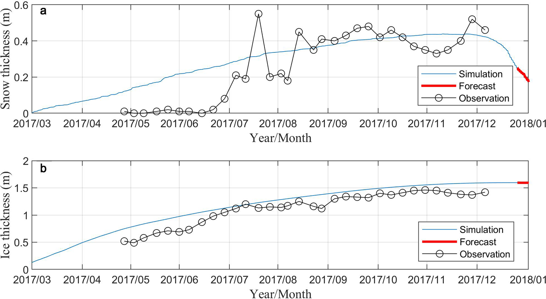
Fig. 10. The simulated (blue lines) and predicted (red lines) snow and ice thickness as well as the observed values (black dots) at the SIP site.
The MODIS image, AMSR2 SIC and FIPS modeled ice mass-balance components in the FIPS domain are shown in Figure 11. The AMSR2 overestimated the fast ice edge compared with the MODIS image. The predicted weekly mean snow and ice thickness were 0.3–0.5 and 1.2–1.6 m, respectively. The load capacity of the combined snow and ice cover was sufficient for transport by snowcats. A 0.4 m ice thickness was considered safe for a person on a skidoo, and 1.2 m ice for snowcats (personal communication from R/V Xuelong Captain, Quan Shen, 2012). The predicted total snowmelt in the FIPS domain was ~0.15 m. The melting of snow may generate a risk of snowcats getting stuck. The internal ice melt was also modeled although the magnitude was very small. Basal ice melt was not predicted. Based on results in Figure 11, R/V Xuelong was advised to anchor in the eastern part of the FIPS domain, where the modeled snow melt and internal ice melt were limited, and the ice was thicker. The HIGHTSI also provided thickness estimates of snow ice and superimposed ice during the simulation and prediction periods. Snow ice and superimposed ice are mechanically weak because of their granular structure (Massom and other, Reference Massom2001). However, historically in this region, congelation ice has comprised most of the fast ice (He and others, Reference He, Chen and Wu1998; Lei and others, Reference Lei, Li, Cheng, Zhang and Heil2010), thus the impact of the weaker snow ice and superimposed ice was considered but not as the priority factor when designing the transportation route.
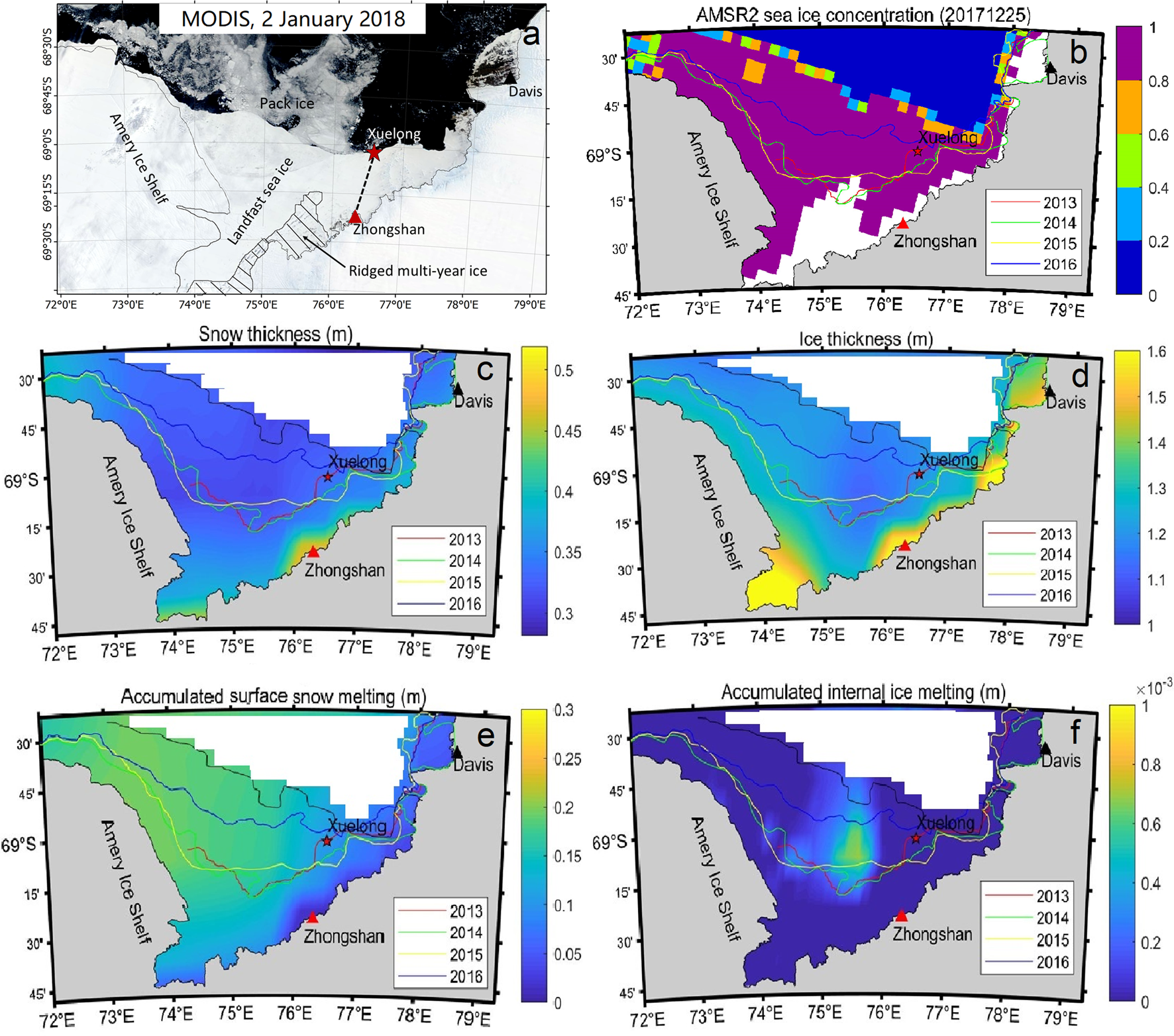
Fig. 11. (a) The MODIS image of fast ice in Prydz Bay on 2 January 2018. (b) AMSR2 SIC on 25 December 2017. The predicted 7 days (25–31 December 2017) FIPS domain mean snow thickness (c); ice thickness (d); accumulated snow surface melting (e) and accumulated internal ice melting (f). The colored lines present the fast ice edge from previous years in the same week in December. The dashed black line in (a) represents the planned transportation route between Zhongshan Station and R/V Xuelong.
In addition, we paid attention to the modeled internal ice melt, which is difficult to measure in the field, but an important consideration for on-ice transport. One may expect that internal ice melt would accelerate once the snow had melted. A large area of internal ice melt occurred to the northwest of the Zhongshan Station (Fig. 11f), which would have contributed to decreasing the load capacity of the sea ice.
To better understand evolution of the fast ice area, the fast ice edge from several previous years for late-December has been marked on the FIPS domain. This information was provided using an automatic satellite-based sea-ice navigation algorithm (Hui and others, Reference Hui2017).
The modeled regional snow thickness indicated that the surface melt started at the front of Amery Shelf, and gradually propagated toward the southeast within the FIPS domain. The modeled snow and ice thickness between Zhongshan and R/V Xuelong were 0.42 ± 0.04 and 1.32 ± 0.20 m, respectively, while the observed snow and ice thickness were 0.58 ± 0.87 and 1.36 ± 0.54 m. The snow surface melt was confirmed by a coastal monitoring system (Fig. 12). HIGHTSI produced internal melt by the end of December because solar radiation is available all day long.
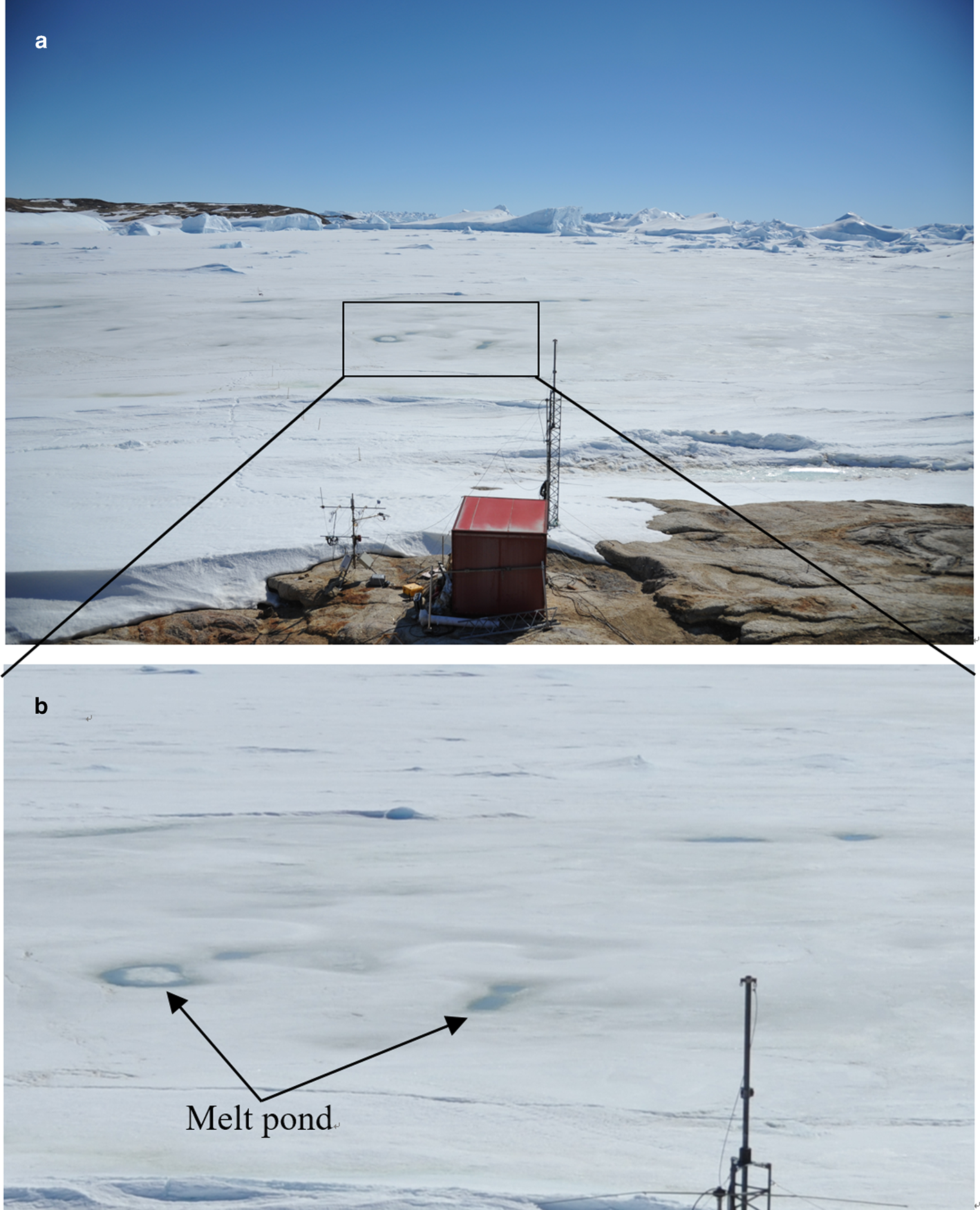
Fig. 12. The surface state of coastal fast ice on 25 December 2017 (a) and surface melt can readily be detected (b).
The simulation results provided by FIPS, in particular the snow and ice prediction, were used to select the transportation route. The R/V Xuelong Captain and crew were satisfied with FIPS service results for 2017/18 season for the successful on-ice route selection from the vessel to the station.
5. Discussion and conclusion
For the last three decades, logistic supplies have been delivered to Zhongshan Station across the fast ice every year during early austral summer by the icebreaker R/V Xuelong. Here we presented results for a FIPS. Sea-ice extent, concentration, ice edge and tide cracks, obtained automatically from satellite remote-sensing data (Hui and others, Reference Hui2016, Reference Hui2017), were used to initialize the snow/ice thermodynamic model HIGHTSI, which uses ECMWF ERA-Interim reanalysis and HRES 10-day forecasts as atmospheric forcing to simulate and predict snow and ice thickness. The products of FIPS are mainly used for planning of the on-ice transportation route from R/V Xuelong to the Zhongshan Station.
Validation from the SIP in 2015 confirmed that the simulations forced by ECMWF ERA interim reanalysis and HRES 10-day forecasts produced useful predictions of snow and ice thickness for the near-coastal Prydz Bay. About 10% overestimation of ice thickness at SIP site was due to the cold bias of ECMWF air temperature, while the modeled maximum ice thickness in the FIPS domain agreed with field measurements (Lei and others, Reference Lei, Li, Cheng, Zhang and Heil2010; Zhao and others, Reference Zhao2019a). Temporal variation of snow accumulation was not captured by HIGHTSI because snowdrift was not considered. However, the annual maximum snow thickness and timing of snow melt were modeled and predicted well.
Close to the coastline of Prydz Bay, snow is largely drifted away by strong wind, but further away from shoreline, snow is accumulated significantly on fast ice, and contributes to ice mass balance at the snow–ice interface. This has been demonstrated by observations and model experiments (Zhao and others, Reference Zhao2019b). The thick snow cover and negative freeboard in 2015 resulted in snow ice formation. Snow ice contributed 30% to the total ice thickness during the growth season because of sea water flooding. While superimposed ice contributed ~20% to the total ice thickness over the melt season because of surface snow melting. Thick snow ice and superimposed ice generally have a weak load capacity when compared to congelation ice. The heavily loaded cargo snowcats are likely to get stuck in soft snow surface and slush.
The FIPS operational service was tested for the 2017/18 ice season. FIPS predicted the congelation ice to make ~85% of the total ice thickness. The exact date for logistic ground transportation largely depends on local ice conditions in November and December. The identification of areas with potential surface melt is important for on-ice transportation. HIGHTSI identified surface and subsurface melting that occurred in the western part of FIPS domain. Depending on the timing of logistic support, the information on snow surface and sub-surface melt is very important for transportation route planning. In general, HIGHTSI has been found good in reproducing the observed onset of snow melt (Cheng and others, Reference Cheng2014).
In the 2017/18 ice season, the FIPS captured very well the maximum snow thickness, the onset of snow melt at the surface, and especially the evolution of ice thickness. The weekly mean forecast for the last week of December suggested a strong snow surface melt across the model domain and apparent internal ice melt northwest off Zhongshan Station. The snow surface melt was confirmed by photos taken nearshore on 25 December 2017 (Fig. 12). Dark surface in early summer can also be upward brine percolation (Maksym and others, Reference Maksym and Jeffries2000). Brine percolation for columnar sea ice needs a high brine volume of ~5% (Golden and others, Reference Golden, Ackley and Lytle1998) and usually occurred for the SYI/MYI. It may not be the case for this study, because the fast ice in Prydz Bay is mostly FYI, thus the in-ice brine channels may not have fully developed. Internal snow and ice melt likely affected the load capacity and, hence, raised the risk for on-ice transport across the fast ice. Hence, the captain of Xuelong and leader of CHINARE finally selected a route over the northeastern section off Zhongshan Station, where less surface melt had occurred than in other parts of the model domain. FIPS was appreciated for providing essential 2-D information of fast ice properties, especially the internal ice melting, which cannot be detected visually.
Ice concentration remained rather constant in the FIPS domain for one duration of operational forecast, as we used a week in this study. Opening of leads and dynamic deformation of ice are limited by the unique coastal and bathymetric geography of the region. For this reason, we used the thermodynamic model to simulate snow and ice evolution, while the dynamic processes, like tidal cracks, coastal polynyas and deformed ice locations, were identified by remote-sensing observations.
In order to further improve the quality of the FIPS service, our attention will focus on improving remote-sensing data to identify properties of the fast ice cover (Karvonen, Reference Karvonen2018). We also plan to apply multi-source reanalysis products to improve the representation of precipitation during the initial simulation preceding the start of FIPS prediction. In Prydz Bay, knowledge of the oceanic heat flux is important for the energy budget of sea ice and, hence, for sea-ice growth (Guo and others, Reference Guo, Shi, Gao, Tamura and Williams2019). In the current FIPS configuration, the temporal variation of F w is based on field observations and model analyses. As the spatial variation of F w in Prydz Bay remains unknown, an acoustic doppler velocity meter for direct measurement of the oceanic heat flux will be deployed underneath the fast ice near the Zhongshan Station during the 2020/21 field season. A snow and ice mass-balance buoy will be deployed to monitor snow and ice thickness in real time (Liao and others, Reference Liao2018). These new measurements are expected to improve the performance of FIPS with respect to snow and ice mass balance.
Acknowledgement
This study was supported by the Natural Science Foundation of China (41876212, 41911530769, 41676176 and 41941009) and the Academy of Finland under Contract 304345. PH was supported by the Australian Government through Australian Antarctic Science projects 4301, 4390 and 4506, and the International Space Science Institute grant no. 406. This is a contribution to the Year of Polar Prediction (YOPP), a flagship activity of the Polar Prediction Project (PPP), initiated by the World Weather Research Programme (WWRP) of the World Meteorological Organisation (WMO). We acknowledge WMO WWRP for its role in coordinating this international research activity. AMSR2-derived sea-ice concentration is courtesy of the University of Bremen (https://seaice.uni-bremen.de/sea-ice-concentration/). MODIS and SAR images were accessed via websites https://worldview.earthdata.nasa.gov/?p=antarctic and https://www.polarview.aq/antarctic, respectively. We are grateful for comments by two anonymous reviewers and editors David Babb and Hester Jiskoot, who helped to significantly improve the manuscript.


 Open access