


1. INTRODUCTION
Glaciers have been considered one of the most significant indicators of climate change over recent decades (IPCC, 2013). Most glaciers around the world have retreated significantly as a result of recent climate change (Bolch and others, Reference Bolch2012; Guo and others, Reference Guo2015), leading to rises in modern sea levels (Gregoire and others, Reference Gregoire, Payne and Valdes2012; Jacob and others, Reference Jacob, Wahr, Pfeffer and Swenson2012; Gardner and others, Reference Gardner2013) and influencing regional hydrological processes in glaciated catchments (Radić and Hock, Reference Radić and Hock2014; Zhang and others, Reference Zhang, Hirabayashi, Liu and Liu2015b).
Alongside global climate change, different types of glaciers in different regions show different responses to variations within regional and local climatic regimes. In general, monsoonal maritime glaciers on the Tibetan Plateau (TP) are more sensitive to climate change, and in particular to fluctuations in temperature (Shi and Liu, Reference Shi and Liu2000; Yao and others, Reference Yao2012; Zhang and others, Reference Zhang, Hirabayashi and Liu2012; Yang and others, Reference Yang2013; Zhu and others, Reference Zhu2017). However, continental glaciers retreat more slowly (Shi and Liu, Reference Shi and Liu2000; Yao and others, Reference Yao2012), with a few glaciers even bucking the trend and advancing (Gardelle and others, Reference Gardelle, Berthier and Arnaud2012a; Jacob and others, Reference Jacob, Wahr, Pfeffer and Swenson2012).
The glaciers on the Gongga Mountains (GGM), on the southeastern margins of the TP, are monsoonal temperate glaciers. Pan and others (Reference Pan2012) determined the extent and rapidity of the change in glacier cover in this area using multi-sourced topographic maps and remote-sensing data. Numerous studies have mentioned the potentially important effects on hydrology of changes in glacier coverage in the GGM as a factor in regional climate change (Li and others, Reference Li2010; Pan and others, Reference Pan2012). Compared to changes in glacier coverage and length, which can be derived relatively easily from remote-sensing data (Paul and others, Reference Paul, Huggel and Kääb2004; Bolch and others, Reference Bolch, Menounos and Wheate2010), changes in glacier thickness are more directly related to changes in a region's glacier mass balance and hydrology (Pieczonka and others, Reference Pieczonka, Bolch, Junfeng and Liu2013).
Debris-covered glaciers are frequently found in high altitude mountain ranges (Juen and others, Reference Juen, Mayer, Lambrecht, Han and Liu2014). Most glaciers in the GGM are covered by layers of debris. Supraglacial debris cover influences glacier terminus dynamics and can thereby modify a glacier's length response to climate change (Scherler and others, Reference Scherler, Bookhagen and Strecker2011). Thin layers of debris or small single grains absorb more heat than ice, due to their lower albedo. The transfer of this energy into the underlying ice increases ablation rates. However, thicker supraglacial debris cover acts as a protective carapace, insulating the underlying ice and significantly reducing ablation rates (Østrem, Reference Østrem1959; Juen and others, Reference Juen, Mayer, Lambrecht, Han and Liu2014).
Despite the apparent importance of direct mass-balance measurements, only a few records exist for the GGM (e.g. Zhang and others, Reference Zhang, Fujita, Liu, Liu and Nuimura2011) due to the inaccessibility of the area and the attendant high labor costs (Ye and others, Reference Ye2015). Fortunately, remote sensing allows the detection of one or several glacier mass changes at a time through multi-temporal surface digital terrain difference analysis (‘the geodetic method’), even in remote mountainous or otherwise unreachable terrains (Paul and Haeberli, Reference Paul and Haeberli2008). For example, this geodetic method can allow DEMs from the 1950s to the 1980s to be digitized from topographic maps (Xu and others, Reference Xu, Liu, Zhang, Guo and Wang2013; Wei and others, Reference Wei2015). Many scholars have also used declassified KH-9 data to derive DEM values for the 1970s (Pieczonka and Bolch, Reference Pieczonka and Bolch2015; Shangguan and others, Reference Shangguan2015). Compared to the inevitable historical limitations of such data, satellite imaging techniques such as SPOT HRV (Berthier and Toutin, Reference Berthier and Toutin2008; Pieczonka and others, Reference Pieczonka, Bolch, Junfeng and Liu2013), ASTER Terra (Willis and others, Reference Willis, Melkonian, Pritchard and Rivera2012; Melkonian and others, Reference Melkonian, Willis, Pritchard and Stewart2016) and ALOS PRISM (Frey and others, Reference Frey, Paul and Strozzi2012; Ye and others, Reference Ye2015) can be used for terrain analysis. In 2012, China launched its own ZY-3 earth observation satellite able to provide stereo pairs for DEM generating. In addition, GLAS/ICESat and SRTM data have often been used in glacier coverage reconstructions (Bolch and others, Reference Bolch2013; Neckel and others, Reference Neckel, Kropáček, Bolch and Hochschild2014). The data from remote sensing is very important for us to understanding the glacier mass-balance change on the TP.
The objectives of this study were to: (1) update decadal-scale changes in glacier coverage using newly-derived boundary data for glaciers from 1966 to 2015; (2) determine any changes in glacier volume and derived mass in the GGM during different time periods using geodetic methods based on a DEM analysis of topographic maps, as well as SRTM, ICESat and ZY-3 data; and (3) investigate the role of debris cover in glaciers mass change in the GGM.
2. STUDY AREA
In 1966, the first Chinese Glacier Inventory (CGI) (Shi, Reference Shi2008) recorded the GGM region on the southeastern margins of the TP (29–30°N, 101–102°E) (Fig. 1) as having 74 glaciers with a total area of 257.7 km2. Most (68%) of the glaciers are covered with debris and the total debris-covered area is ~32 km2 (13.5% of the total glacier area of the region (Zhang and others, Reference Zhang, Hirabayashi, Fujita, Liu and Liu2016)). The debris is relatively thin in the upper ablation zones. As the elevation decreases, the debris thickness increases (Zhang and others, Reference Zhang, Fujita, Liu, Liu and Nuimura2011). The glaciers in the GGM are monsoonal temperate glaciers, and are therefore characterized by high flow velocities (~170 m a−1 at 3600 m a.s.l.), high accumulation rates and intense melting (~6000 mm at 3600 m a.s.l.) (Su and others, Reference Su, Song and Cao1996). Mean annual precipitation (MAP) in this region is ~1930 mm at an altitude of 3000 m a.s.l. on the eastern slopes of the GGM, where the mean annual air temperature (MAT) is ~3.9 °C. According to the record form Gonggasi meteorological station, from May to September, the precipitation accounts for 80% of the whole year (Su and others, Reference Su, Song and Cao1996). At an elevation of 3700 m a.s.l. on the GGM's western slopes, MAP is ~1150 mm and MAT is ~2.2 °C (Zhang and others, Reference Zhang2015a). The equilibrium-line altitude values are ~4900 and 5100 m a.s.l. for the eastern and western slopes of the GGM, respectively (Shi, Reference Shi2008). It has been calculated using multi-temporal remote-sensing images (Pan and others, Reference Pan2012) that the glaciers in the GGM region shrank by ~29.2 km2 during the period 1966–2009.

Fig. 1. Location and topography of the Gongga Mountains (GGM). Background: SRTM; glacier outlines based on first CGI. The orange and pink boxes show ZY-3 data coverage from 21 March 2012 and 23 December 2015 respectively.
3. DATA SOURCES AND METHODS
3.1. Historical topographic maps
Topographic maps can provide details of glacier surface topography and have been widely used for glaciological purposes (Wei and others, Reference Wei2015). In this study, two topographic maps from 1966 plotted using a scale of 1:100 000, and four topographic maps from 1989 plotted using a scale of 1:50 000, and subsequently acquired by the State Bureau of Surveying and Mapping (Table 1), were used for glacier terrain analysis. We digitized the 20 or 40 m interval contours and spot heights to generate a triangular irregular network map to produce DEM values for the years 1966 and 1989, using the Beijing 1954 datum. Subsequently, the DEMs were re-projected to the UTM coordinate system on the basis of WGS84 datum so as to keep them consistent with other satellite images. During the projection, a seven-parameter datum transformation model with a 30 m resolution was used (Cao and others, Reference Cao2014). Since the mean slope of the glacierized areas in the GGM is 23°, in accordance with national photogrammetrical mapping standards, the nominal vertical accuracy of these topographic maps with 1:50 000 and 1:100 000 were better than 8 and 16 m, respectively, for the mountainsides and high mountain areas (with slopes between 6° and 25°) (GB/T12343.1-2008; SAC, 2008).
Table 1. Utilized input and reference datasets

3.2. SRTM DEM and ICESat GLAS data
The SRTM acquired interferometric synthetic aperture radar (InSAR) data simultaneously in both the C- and X-band frequencies from 11 to 22 February 2000 (Farr and others, Reference Farr2007). The X-band SAR system was operated with a narrower scan width of only 45 km, leaving large data gaps in the resulting X-band DEM. Such DEM data can be taken as representative of the elevation of glacier surfaces after the 1999 ablation period, with slight seasonal variances (Gardelle and others, Reference Gardelle, Berthier, Arnaud and Kääb2013; Pieczonka and others, Reference Pieczonka, Bolch, Junfeng and Liu2013; Shangguan and others, Reference Shangguan2015). Fortunately, the entire study region (GGM) was covered by the SRTM X-band. Therefore, in this study, the SRTM X-band was used in order to avoid penetration problems in SRTM C-band by assuming that the penetration depth of the SRTM X-band beam into snow and ice was zero (Gardelle and others, Reference Gardelle, Berthier and Arnaud2012a).
ICESat Global Land Surface Altimetry data products (Zwally and others, Reference Zwally2002; Neckel and others, Reference Neckel, Kropáček, Bolch and Hochschild2014) provided by the National Snow and Ice Data Center (NSIDC) were also introduced into this study. The height provided in the ICEsat GLAS14 was converted to orthometric height using the same reference as the SRTM DEM (referred toWGS84 Ellipsoid and EGM96 Geoid). Bilinear interpolation was used to extract the SRTM surface elevation at the location of each ICESat measurement. The elevation difference (dh) between each ICESat estimate and SRTM DEM represents the thickness change at the sampled footprint. Similar to previous studies, a threshold of 150 m was applied to filter obvious errors of dh due to cloud cover and atmospheric noise (Kääb and others, Reference Kääb, Berthier, Nuth, Gardelle and Arnaud2012; Neckel and others, Reference Neckel, Kropáček, Bolch and Hochschild2014; Ke and others, Reference Ke, Ding and Song2015).
The accuracy of ICESat elevation footprints has been established as ~10 cm for flat surfaces (Zwally and others, Reference Zwally, Yi, Kwok and Zhao2008), but is lower for inclined surfaces (Wang and others, Reference Wang, Yi and Sun2017). We quantify the combined uncertainty in height change measurements in Section 3.5.
3.3. ZY-3 DEM data
The ZY-3 satellite was launched in 2012 carrying three stereo pair cameras (Forward, Backward, Nadir) with a resolution of 3.5/2.1 m. We collected ZY-3 stereo pair images of two phases (21 March 2012 and 23 December 2015) and then generated the DEM of the study area using the ‘DEM Extraction’ Model provided by the ENVI 5.0 software, using the geographic reference system WGS84 UTM, Zone 47 N. During the DEM generation, at least 20 Ground Control Points (GCPs) for each ZY-3 image were selected. Their coordinates and altitudinal values were derived from Landsat 8 scenes and the DEM data for 1989. Similarly to the SRTM data, the DEM data from the 21 March 2012 ZY-3 images were taken as representative of glacier surface altitudes toward the end of the 2011–2012 accumulation season; the DEM data from the 23 December 2015 ZY-3 images were taken to be indicative of glacier surface altitudes after the 2015 ablation period.
3.4. Glacier boundary inventory and glacier mass change
Pan and others (Reference Pan2012) conducted a systematic study of the glacier coverage in the study area from 1966 to 2009. In this study, we obtained ZY-3 satellite images for 2015 prior to conducting geometric correction and ortho-rectification. Glacier boundaries were digitized using manual methods, and repeatedly verified using imagery in Google Earth.
Changes in glacier surface elevation above sea level were calculated based on area-averaged value per 100 m of elevation, using DEM differencing (Xu and others, Reference Xu, Liu, Zhang, Guo and Wang2013; Shangguan and others, Reference Shangguan2015; Wei and others, Reference Wei2015).
3.5. DEM co-registration and accuracy
Multi-temporal DEMs require a co-registration to remove the horizontal and vertical offsets before any differential analysis can be performed (Pieczonka and others, Reference Pieczonka, Bolch, Junfeng and Liu2013). An analytical method proposed by Nuth and Kääb (Reference Nuth and Kääb2011) and later proven as effective by Paul and others (Reference Paul2015) was used in this study. All DEMs were bi-linearly resampled to the same cell size of 30 m, and in order to optimize the registration, the observed relationship between DEM altitude differences and aspect in off-glacier areas were used to make further relative adjustments (Fig. 2). Some iterations were built into the registration process where necessary. Extreme outliers were not taken into account and were removed using a threshold method (Berthier and others, Reference Berthier, Schiefer, Clarke, Menounos and Rémy2010; Gardelle and others, Reference Gardelle, Berthier, Arnaud and Kääb2013). The statistical characteristics evident in these altitudinal differences were used to exclude the pixels that represent altitudinal differences outside the 5–95% range, so as to correct for potential bias (Pieczonka and others, Reference Pieczonka, Bolch, Junfeng and Liu2013; Wei and others, Reference Wei2015). Details of the shifts and errors observed after the abovementioned adjustments were made are listed in Table 2.

Fig. 2. Scatter plot of slope-standardized altitudinal differences in terrain aspect for off-glacier areas. (a) Before co-registration; and (b) after co-registration (but before optimization using slope aspect).
Table 2. Shift vectors in directions x, y and z (Master DEM > Slave DEM), and uncertainties inherent within non-glaciated areas

AD, mean elevational difference, STD, std dev.
We found that even after linear shifting in x, y and z, there is still some obvious elevation difference. As pointed out by previous studies (Berthier and others, Reference Berthier, Arnaud, Vincent and Rémy2006; Gardelle and others, Reference Gardelle, Berthier and Arnaud2012b), elevation-dependent vertical bias in mountainous regions is attributable to differences in the original spatial resolution of the two DEMs. The coarse DEM is prone to underestimate the heights of the sharp peaks or ridges with high terrain curvature due to its limited capacity of the representation of high-frequent changes in slopes. This bias can be corrected by the relationship between elevation difference and maximum curvature over the stable terrain off glaciers (Gardelle and others, Reference Gardelle, Berthier and Arnaud2012b, Reference Gardelle, Berthier, Arnaud and Kääb2013). A clear polynomial relationship is found between the two variables, and thus in this study, a three-degree polynomial fitting is utilized to make the correction (Fig. 3).

Fig. 3. Relationship between elevation difference and maximum curvature.
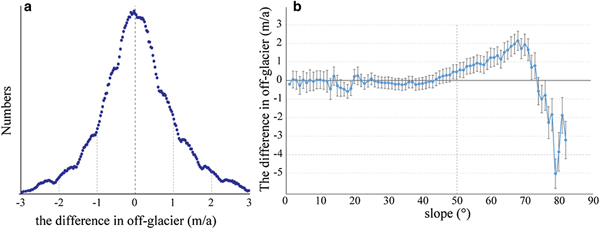
After the adjustments, the off-glacier errors are mostly distributed between −1 and 1 m/a (Fig. 4a) and that the large errors are found on steep slopes >50° (Fig. 4b) and therefore do not affect the glacier height change measurements. Then, we estimated the uncertainty in the differences between each pair of DEMs by using the normalized median absolute deviation (expressed by 1.4826 × MED $\lpar {\vert {\tilde{x}-x_i} \vert } \rpar $|; x i: elevation difference; $\tilde{x}$: median) (Höhle and Höhle, Reference Höhle and Höhle2009; Shangguan and others, Reference Shangguan2015; Zhang and others, Reference Zhang2018) for the non-glaciated areas (Table 2).

Fig. 4. The final histograms of the difference in off-glacier (a), and the relationship between elevation difference in off-glacier and slope (b).
To convert elevation change to mass change, an assumption is required about ice density. A density of 850 ± 60 kg m−3 was used (cf. Huss, Reference Huss2013). The final mass-balance uncertainty (E) was calculated as (Zhang and others, Reference Zhang2018):
 $$E = \; \sqrt {{\left( {\displaystyle{{{\rm NMAD}} \over t} \times \displaystyle{{\Delta \rho} \over {\rho_{\rm W}}}} \right)}^2 + {\left( {\displaystyle{{{\rm NMAD}} \over t} \times \displaystyle{{\rho_{\rm I}} \over {\rho_{\rm W}}}} \right)}^2} $$
where t is the observation period, ρ I the ice density (850 kg m−3), Δρ the ice density uncertainty (60 kg m−3), ρ W the water density (999.92 kg m−3) (Pieczonka and Bolch, Reference Pieczonka and Bolch2015; Zhang and others, Reference Zhang2018).
4. RESULT
4.1. Changes in glacier coverage in the GGM
Pan and others (Reference Pan2012) found that glacier coverage in the GGM had shrunk from 257.7 km2 in 1966 to 228.5 km2 in 2009. Our study confirms that the glaciers in this region continued to retreat to a total coverage of ~224.7 km2 in 2015. From 1966 to 2015, glacier coverage decreased by 33.0 km2 (Fig. 5a). Glacier area on the east and west slopes of the GGM decreased by 11.7 and 13.6% since 1966, respectively.

Fig. 5. (a) Glacier boundaries in the GGM for 1966, 1974, 1989, 1994, 2005, 2009 and 2015. (b) Scatter plot of initial glacier area in 1966 versus area loss as a percentage of this initial glacier area between 1966 and 2015. (c) Glacier area at different median altitudes for 1966 and 2015. (d) Area loss in different median altitudes.
The percentage and rate of area loss were greater for smaller glaciers than for the larger glaciers. A non-linear relation was found between the initial glacier area and glacier area loss as a percentage of this initial glacier area (Fig. 5b). Furthermore, the maximum percentage glacier area loss of ~40% occurred below 4000 m a.s.l., and as elevation increased, this percentage decreased. Conversely, the actual size of glacier area loss, due to the distribution of glaciers in this region, was found be greater at higher altitudes, with the maximum area loss occurring in the 4900–5100 m band (Figs 5c, d). Above this altitude, the amount of area loss decreased as altitude increased. What is more, when the altitude reached ~5900 m a.s.l., the amount of glacier area loss and the glacier area loss percentage both fell to 0, indicating that the study area's glaciers that are found at altitudes of >5900 m a.s.l. remained relatively stable between 1966 and 2015.
4.2. Changes in glacier surface elevation
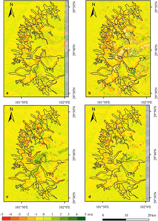
Most of the glaciers in the region appear to show a significant surface lowering in ablation region of −26.7 ± 2.03 m (−0.54 ± 0.04 m a−1) for the 1966–2015 period (Fig. 6), with an average of −0.51 ± 0.04 and −0.60 ± 0.04 m a−1 on the east and west slopes, respectively. Glacier mass decreased by 6.08 ± 0.53 km3 w.e. in the study area, although the glacier thickness reduction rate was not consistent over different time periods. Generally speaking, the glacial thinning rate in the GGM is accelerating. During the 1966–1989 period, the glacier mass budget was −0.31 ± 0.06 m w.e. a−1; during the 1989–1999 period, it was −0.51 ± 0.04 m w.e. a−1; and during the most recent 1999–2015 period, it rose to −0.65 ± 0.10 m w.e. a−1 (Table 3).

Fig. 6. Differences in glacier surface elevation above sea level over time periods of different lengths, after relative adjustments: (a) 1966–1989; (b) 1989–1999; (c) 1999–2015; and (d) 1966–2015. The large errors visible in the DEM difference figures are found on steep slopes (see Fig. 4).
Table 3. Glacier mass changes in the GGM, 1966–2015

Determining the factors which control glacier ablation is more difficult, as, along with melt mode, they are highly complex, and produce different levels of melt in different areas. As a general rule, glacial thinning is at its maximum at low elevations, and at its minimum at higher altitudes (Barrand and others, Reference Barrand, James and Murray2010). The lower elevation segments of GGM glaciers have a relatively high melt rate, averaging −0.81 ± 0.04 m a−1 below 5000 m a.s.l. for the period 1966–2015. Comparing ICESat and SRTM data, the mean loss of glacier was 0.50 ± 0.18 m w.e. a−1 for the period 1999–2009 (Table 4).
Table 4. Changes in GGM glacier elevation using ICESat data in comparison with SRTM data

Supraglacial debris cover may influence loss of glacial mass in glacier ablation region. In the GGM, 68% of the region's glaciers are debris-covered, where the debris-covered proportions of total glacier area vary from 1.74 to 53.0% (Zhang and others, Reference Zhang, Hirabayashi, Fujita, Liu and Liu2016). Using Google Earth imagery, a secondary CGI and the data from Zhang and others (Reference Zhang, Hirabayashi, Fujita, Liu and Liu2016), we reconstructed a debris-covered glacier map of the GGM (Fig. 7). The rate of change in the mean glacier surface altitude was −0.54 ± 0.04 m a−1 over the 1966–2015 period in the study area. The areas where debris-covered glaciers predominate experienced a rate of change of −0.94 ± 0.04 m a−1 in 1966–2015. Almost all the debris-covered glaciers in the GGM are distributed at <5000 m a.s.l. However, the rate of change in the mean surface elevation for debris-free glaciers found at similar elevations was ~ −0.78 ± 0.04 m a−1. It is therefore reasonable to assume that glacial debris cover in the GGM may exert an accelerated effect on glacier melt similar to that found by Zhang and others (Reference Zhang, Hirabayashi, Fujita, Liu and Liu2016).

Fig. 7. Spatial distributions of debris-covered glaciers in the Gongga Mountains where glacier surface altitudes are <5000 m a.s.l.
5. DISCUSSION
From 1966 to 2015, glacier mass loss in the GGM was −0.46 ± 0.04 m w.e. a−1. This result represents a similar result to that found by Zhang and others (Reference Zhang, Hirabayashi and Liu2012), who recorded a mean loss in glacier thickness of −0.42 m w.e. a−1 in the Hailuogou catchment using an energy mass-balance modeling method for the period 1952–2009. Our result shows that glacier thickness at low elevations changes at a rate of 0.81 ± 0.04 m a−1, which was similar to the GPS observation results recorded by Zhang and others (Reference Zhang, Fujita, Liu, Liu and Wang2010) and Zhang and others (Reference Zhang2015a).
We compared ICESat and SRTM data to obtain a mean glacier elevation change rate of −0.50 ± 0.18 m w.e. a−1 for the period from 1999 to 2009. According to analyses of ICESat data employed in this study, the glacier elevation change rate observed is larger than that seen in the Hengduan Mountains (i.e. −0.40 ± 0.41 m a−1, Gardner and others, Reference Gardner2013), and slightly smaller than that of −0.69 ± 0.36 m w.e. a−1 than observed in the eastern Nyainqentanglha range (a range of the Hengduan Mountains) (Neckel and others, Reference Neckel, Kropáček, Bolch and Hochschild2014).
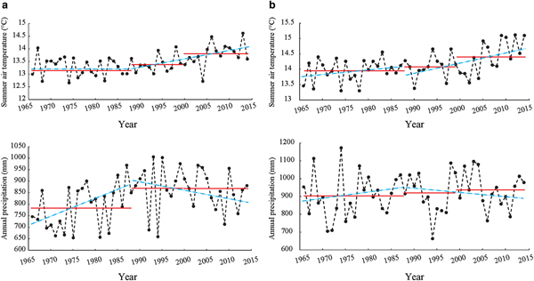
Factors that affect glacier change include both external (climatic) and internal (debris cover, glacier size, topography, etc.) controls. Zhang and others (Reference Zhang2015a) pointed out that it is most likely that climate change has led to the retreat of the GGM's glaciers from 1966 until the present day. Though precipitation values increased over the period, it cannot have fully offset the impact on glacier melt caused by rising temperatures (Fig. 8).

Fig. 8. Changes in annual summer (June to August, inclusive) air temperature and annual precipitation values derived from the (a) Kangding and (b) Jiulong meteorological station datasets. The red line represents the mean value for the different time periods; the blue dashed line is the linear trend line.
During the first period of study (1966–1989), precipitation in the GGM increased, while temperature values remained essentially unchanged. During the next period (1989–2015), precipitation decreased, while the temperature increased at a faster rate than previously (Fig. 8). Therefore, the glacier thinning rate in the period 1989–2015 was larger than over the period 1969–1989. The accelerating glacier thinning rate from 1966–1989 to 1989–1999 and to 1999–2015 may be caused by the mean temperature of these three periods continuing to rise (Fig. 8).
Supraglacial debris may influence any modeling of glacier melt. Zhang and others (Reference Zhang, Hirabayashi and Liu2012) proposed that supraglacial debris markedly accelerates any loss in glacier mass, while Juen and others (Reference Juen, Mayer, Lambrecht, Han and Liu2014) concluded that melt rates below debris thicker than ~0.1 m are highly reduced, as the ice is shielded by the debris cover. Zhang and others (Reference Zhang2015a) pointed out that the inhomogeneity of debris thickness can lead to a complex pattern of glacier melt, and that there is hence no obvious relation between changes in glacier surface and glacier altitude in debris-covered areas. With reference to our results, however, we would propose that, for the whole of the GGM at least, supraglacial debris appears to play a positive role in promoting glacier melt.
6. CONCLUSION
In this study, we analyzed changes in glacier mass in the GGM region using topographic maps (i.e. for 1966 and 1989), ZY-3 images (i.e. for 2015) and a cross-comparison of ICESat and SRTM datasets. The results showed that glacier coverage in the GGM region has been decreasing since 1966, and that the total glacier coverage of 224.7 km2 observed for 2015 represents a reduction of 33 km2, or 12.8%. From 1966 to 2015, the surface altitude of glaciers in the GGM decreased by −26.7 ± 2.03 m (0.54 ± 0.04 m a−1). During the 1969–1989 period, the rate of change in glacier thickness was −0.37 ± 0.07 m a−1; this rate of change was −0.60 ± 0.05 m a−1 for the period 1989–1999; and for the most recent period, i.e. 1999–2015, the rate of change in glacier thickness was −0.76 ± 0.12 m a−1. As a general rule, glacier melt rates were higher at lower elevations than at higher elevations in this region. Additional analysis suggested that the supraglacial debris coverage of glaciers in the GGM region likely promoted glacier melt.
ACKNOWLEDGEMENTS
We thank two anonymous reviewers and scientific editor Hamish Pritchard for valuable insights that greatly strengthened the manuscript. This study was financially supported by the National Natural Science Foundation of China (grant No. 41701057), the Ministry of Science and Technology of the People's Republic of China (grant No. 2013FY111400), and Fundamental Research Funds for the Central Universities (lzujbky-2018-kb33; lzujbky-2017-225).


 Open access