2. Theoretical model

We consider an infinitely long cylindrical TC set-up consisting of inner and outer cylinders with radii $r_{in}$ and $r_{out}$ rotating with angular velocities $\varOmega _{in}$ and $\varOmega _{out}$ in the cylindrical coordinates $(r, \phi, z)$ corresponding to the PROMISE set-up (figure 1). In the absence of endcaps, the equilibrium azimuthal flow $u_{0\phi }=r\varOmega (r)$ between the cylinders has a classical hydrodynamical TC profile of angular velocity $\varOmega (r)=S_1+(S_2/r^2)$, where $S_1=\varOmega _{in}(\mu -\eta _{\varOmega }^2)/(1-\eta _{\varOmega }^2)$ and $S_2=\varOmega _{in}(1-\mu )r_{in}^2/(1-\eta _{\varOmega }^2)$ with the ratio of the cylinders’ radii $\eta _{\varOmega }=r_{in}/r_{out}$ ($=0.5$ in PROMISE) and angular velocities $\mu =\varOmega _{out} / \varOmega _{in}$. Note that a split-endcaps configuration is used in the PROMISE set-up, which significantly reduces the global Ekman pumping, thereby sustaining this TC profile in the bulk flow to a good approximation (Stefani et al. Reference Stefani, Gerbeth, Gundrum, Hollerbach, Priede, Rüediger and Szklarski2009). A central rod carrying current $I$ produces an azimuthal magnetic field $B_{0\phi }(r)=\mu _0I/(2{\rm \pi} r)$ between the cylinders, where $\mu _0$ is the magnetic permeability of vacuum. Since this current of the order of $10$ kA produces appreciable Ohmic dissipation, $P_{rod}\sim 1$ kW, a water cooling system and a vacuum insulation balance the thermal heating at the centre, see figure 1.

Figure 1. The PROMISE experiment using GaInSn as a working fluid. (a) Cross-section of the experiment with the height ${h=40}$ cm and the inner and outer radii, $r_{in} = 4$ cm and $r_{out} = 8$ cm, of the central TC-cell: (1) vacuum insulation, (2) upper motor, (3) current-carrying copper rod, (4) ultrasound Doppler velocimetry (UDV) sensors, (5) outer cylinder, (6) top acrylic glass split rings, (7) inner cylinder, (8) central cylinder, (9) bottom split rings, (10) bottom motor and (11) interface. (b) Two-dimensional (2-D) sketch of the PROMISE-TC set-up showing heat radiation from the vacuum-insulated current-carrying rod. Heat flux is directed from the inner to outer cylinder with temperatures $T_1$ and $T_2$, respectively, obeying $T_1 > T_2$, which induces convective motion in the fluid. A reverse temperature gradient and hence opposite convective velocities can be set by preheating the outer solenoidal coil before starting the experiment.

The magnetohydrodynamics (MHD) equations for an incompressible fluid with a temperature gradient are

(2.1)$$\begin{gather} \frac{\partial \boldsymbol{u}}{\partial t}+(\boldsymbol{u}\boldsymbol{\cdot}\boldsymbol{\nabla})\boldsymbol{u}={-}\frac{1}{\rho} \boldsymbol{\nabla} p + \frac{\boldsymbol{J}\times \boldsymbol{B}}{\rho}+\nu \nabla^2 \boldsymbol{u} -\boldsymbol{g}\beta \delta T , \end{gather}$$

(2.2)$$\begin{gather}\frac{\partial \boldsymbol{B}}{\partial t}=\boldsymbol{\nabla} \times(\boldsymbol{u}\times \boldsymbol{B})+\eta \nabla^2 \boldsymbol{B}, \end{gather}$$

(2.3a,b)$$\begin{gather}\boldsymbol{\nabla} \boldsymbol{\cdot} \boldsymbol{u}=0, \quad \boldsymbol{\nabla} \boldsymbol{\cdot} \boldsymbol{B}=0. \end{gather}$$

where $\rho$ is the constant density, $\boldsymbol {u}$ is the velocity, $p$ is the thermal pressure, $\boldsymbol {B}$ is the magnetic field, $\nu$ and $\eta$ are, respectively, the fluid kinematic viscosity and magnetic diffusivity and $\boldsymbol {J}=\mu _0^{-1}\boldsymbol {\nabla }\times \boldsymbol {B}$ is the current density. The last term $-\boldsymbol {g}\beta \delta T$ on the right-hand side of (2.1) is the buoyancy force in the Boussinesq approximation driving thermal convection flow (Landau & Lifshitz Reference Landau and Lifshitz1987), where $\beta >0$ is the coefficient of thermal expansion of the fluid, $\delta T=T-T_0$ is the temperature deviation from the reference stationary profile $T_0(r)$ in the absence of convection, which is set by the temperatures $T_1$ and $T_2$ of the inner and outer cylinders, respectively (figure 1). The gravitational acceleration $\boldsymbol {g}=-g\boldsymbol {e}_z$ points opposite the unit vector $\boldsymbol {e}_z$ of the $z$-axis. The background azimuthal magnetic field due to the central current $I$ is written as $\boldsymbol {B_0} = B_0(r_{in}/r)\boldsymbol {e}_\phi$, where $B_0= \mu _0I/(2{\rm \pi} r_{in})$ is the value of this field at $r_{in}$ and $\boldsymbol {e}_\phi$ is the unit vector in the azimuthal direction. In addition, the present set-up of the PROMISE experiment uses an enhanced pentagonal-shaped frame system maintaining an axisymmetry of the background azimuthal field with a relative error $\Delta B_{\phi } / B_{0} < 10^{-2}$.

Apart from being a magnetic field source, the current also represents a heat source, as illustrated in figure 1(b), where the thermal radiation from the Joule heating of the current-carrying central rod transports heat outwards to the inner cylinder (see details in Seilmayer et al. Reference Seilmayer, Ogbonna and Stefani2020). As the inner cylinder's wall heats up, it drives convective motion of the fluid with an axial velocity $u_{0z}$, which is directed upwards along that wall, but downwards along the outer cylinder wall. A heat flux in the opposite direction and hence a reverse convection flow is obtained by preheating the outer solenoidal coil (e.g. by letting current through it) before the start of the experiment. Assuming balance between Lorentz and axial buoyancy forces in a stationary convection flow, Seilmayer et al. (Reference Seilmayer, Ogbonna and Stefani2020) estimated the characteristic axial velocity of this flow as $u_{0z}\approx 0.2\ {\rm mm}\ {\rm s}^{-1}$ at the outer cylinder for a temperature difference $\Delta T\sim 0.1$ K and a current of $I=20$ kA used in those experiments. This velocity is smaller than that of the basic azimuthal TC flow. Thus, the equilibrium flow represents a combination of the main TC flow and the radially varying axial velocity $u_{0z}$, i.e. $\boldsymbol {u}_0=(0, r\varOmega (r), u_{0z}(r))$ with the corresponding pressure profile $p_0(r)$. Due to the small temperature difference, we neglect the thermal effects (i.e. buoyancy term) for perturbations analysed in the next section. In fact, as we will see below, thermal convection influences the dynamics of AMRI primarily through its axial velocity.

2.1. One-dimensional linear stability analysis

We consider small perturbations of velocity $\boldsymbol {u}'=\boldsymbol {u}-\boldsymbol {u}_0$, pressure $p'=p-p_0$ and magnetic field $\boldsymbol {b}'=\boldsymbol {B}-\boldsymbol {B}_0$ about the above equilibrium values, which are functions of the radius $r$ and depend on time $t$, azimuthal angle $\phi$ and axial coordinate $z$ as a normal mode $\propto \exp (\gamma t+{\mathrm {i}} m\phi +{\mathrm {i}} k_z z)$, where $\gamma$ is the (complex) eigenvalue, while $k_z$ and the integer $m$ are the axial and azimuthal wavenumbers, respectively. A positive real part (growth rate) of any eigenvalue, ${\mathcal {R}}(\gamma ) > 0$, indicates the instability of perturbations. We normalize length by $r_{in}$, time by $\varOmega _{in}^{-1}$, $\gamma$ and $\varOmega (r)$ by $\varOmega _{in}$, $\boldsymbol {u}$ by $\varOmega _{in} r_{in}$, $p$ by $\rho r_{in}^2\varOmega _{in}^2$, $\boldsymbol {B_0}$ by $B_0$, and ${ \boldsymbol b}'$ by ${\mathit {Re}}{\mathit {Pm}} B_0$, where ${\mathit {Re}} = \varOmega _{in}r_{in}^2/\nu$ is the Reynolds number and the magnetic Prandtl number $Pm = \nu /\eta =1.4 \times 10^{-6}$ is very small, typical of the working liquid GaInSn in the experiments. We also define another main parameter – the Hartmann number ${\mathit {Ha}} = B_0 r_{in}/\sqrt {\rho \mu _0\nu \eta }$ (${\approx } 7.77 \times I$/kA for GaInSn) characterizing magnetic field strength.

The perturbations of the velocity and magnetic field are divergence-free (2.3), so that they can be split into toroidal and poloidal components (primes will be omitted), $\boldsymbol {u}=\boldsymbol {\nabla }\times (e\boldsymbol {e}_r)+\boldsymbol {\nabla }\times \boldsymbol {\nabla }\times (f\boldsymbol {e}_r)$, $\boldsymbol {b}=\boldsymbol {\nabla }\times (g\boldsymbol {e}_r)+\boldsymbol {\nabla }\times \boldsymbol {\nabla }\times (h\boldsymbol {e}_r)$, where $e,f,g,h$ are the functions of only radius, $\boldsymbol {e}_z$ is the radial unit vector and the operator $\boldsymbol {\nabla }=(\partial /\partial r, {\rm i}m/r, {\rm i}k_z)$. Linearizing (2.1)–(2.2), substituting these representations of the velocity and magnetic field, ignoring the buoyancy force and using the above normalizations, we finally get a system of four coupled one-dimensional (1-D) linear eigenvalue equations (Hollerbach et al. Reference Hollerbach, Teeluck and Rüdiger2010),

(2.4)$$\begin{gather} {\mathit{Re}}\gamma(C_2 e+C_3 f)+C_4 e+C_5 f = {\mathit{Re}} (E_1+F_1) + {\mathit{Ha}}^2 (G_1 + H_1), \end{gather}$$

(2.5)$$\begin{gather}{\mathit{Re}}\gamma(C_3 e+C_4 f)+C_5 e+C_6 f = {\mathit{Re}} (E_2 + F_2) + {\mathit{Ha}}^2 (G_2 + H_2), \end{gather}$$

(2.6)$$\begin{gather}{\mathit{Re}}{\mathit{Pm}}\gamma(C_1 g+C_2 h)+C_3 g + C_4 h = E_3+F_3 + {\mathit{Re}}{\mathit{Pm}} (G_3 + H_3), \end{gather}$$

(2.7)$$\begin{gather}{\mathit{Re}}{\mathit{Pm}}\gamma(C_2 g + C_3 h)+C_4 g+C_5 h = E_4+F_4 + {\mathit{Re}}{\mathit{Pm}} (G_4 + H_4), \end{gather}$$

where the operators $C_n$ are given by $C_n:=\boldsymbol {e}_r(\boldsymbol {\nabla }\times )^n(: \,\boldsymbol {e}_r),\ n\in [1,6]$, while other terms on the right-hand side of these equations are

(2.8)

(2.9)

(2.10)

(2.11)$$\begin{gather}F_3={\rm i}m r^{{-}2} \Delta f, \end{gather}$$

(2.12)$$\begin{gather}F_4={-}{\rm i}k_zr^{{-}2} \hat{\Delta} f , \end{gather}$$

(2.13)

(2.14)

(2.15)

where $\hat {\varDelta }=4m^2 r^{-2}+2k_z^2$ and $\varDelta = m^2 r^{-2}+k_z^2$. The stationary and radially varying axial velocity $u_{0z}(r)$ induced by convection introduces new contributions in several terms $E_1, E_2, F_1, F_2, G_4, H_3, H_4$ compared with the case without convection $(u_{0z}=0)$, which are highlighted in blue. The inner and outer cylinders of the PROMISE device are made of copper (figure 1) and hence conducting boundary conditions are used for the magnetic field, while no-slip conditions for the velocity. The eigenvalue problem posed by (2.4)–(2.7) together with these boundary conditions allow us to determine the eigenvalues $\gamma$ and the associated eigenmodes. To solve this problem, we use the 1-D code of Hollerbach et al. (Reference Hollerbach, Teeluck and Rüdiger2010) based on the spectral collocation method with $N = 30\mbox{--}40$ Chebyshev polynomials, thereby reducing these linear differential equations to a large $4N \times 4N$ matrix eigenvalue equation for $\gamma$ which is then solved with the LAPACK library.

As already noted in the Introduction, following Paper I, in this work we focus on the absolute form of AMRI and, using the procedure described in that paper, identify the corresponding unstable modes that are characterized by zero group velocity (but non-zero phase velocity) in the axial $z$-direction and hence stay inside the TC device. A key feature of these modes is that their axial wavenumber is complex $k_{z,a}={\mathcal {R}}(k_{z,a})+\textrm {i}{\mathcal {I}}(k_{z,a})$, resulting in the increase of mode amplitudes along or opposite the $z$-axis depending on the sign of the imaginary part of the wavenumber ${\mathcal {I}}(k_{z,a})$ (see details in Paper I). The requirement of zero group velocity implies mathematically that the wavenumber $k_{z,a}$ should be a saddle point of the dispersion relation $\gamma (k_z)$, where its complex derivative is zero, $\partial \gamma (k_z)/\partial k_z|_{k_z=k_{z,a}}=0$. From this condition we determine $k_{z,a}$ and then calculate the corresponding growth rate $\gamma _a={\mathcal {R}}(\gamma (k_{z,a}))$ for different $Ha$ and $Re$.

Note that the axial velocity of convection, $u_{0z}$, its radial shear, $u_{0z}'$ and the azimuthal wavenumber $m$ enter (2.4)–(2.7) as products $mu_{0z}$ and $mu_{0z}'$ in the right-hand side terms of these equations, which thus introduce asymmetry with respect to $m$ – the selection of $m=1$ or $m=-1$ AMRI-unstable modes. As is shown below, this selection effect primarily manifests itself in the enhancement of the growth rate of either of these two modes and lowering (or even suppressing) the other.

2.2. Temperature profile

So far, the mathematical expression of the axial velocity $u_{0z}$ has been kept arbitrary, i.e. in principle it may have any radial dependence and can, therefore, be explored over a broad range of parameter space in $B_0$ and $\varOmega _{in}$ which may be of astrophysical interest. However, finding an exact form of an established stationary $u_{0z}$ in the given cylindrical annulus of a TC flow bounded by endcaps due to the combined action of buoyancy, inertia and the imposed azimuthal field is another problem, which we do not address here. Instead, we adopt its simplified model – infinitely long rotating cylinders in the presence of a radial temperature gradient and a current-free azimuthal field. Since $Pm \ll 1$, the effect of the Lorentz force on the convective motion is small. In this case, an exact stationary axisymmetric solution of momentum equation (2.1) was found by Ali & Weidman (Reference Ali and Weidman1990) that consists of a TC flow $u_{0\phi }=r\varOmega (r)$ and the convection axial velocity given by

(2.15)\begin{align} u_{0z}=\frac{A_{0z}}{(1-\eta_\varOmega)^2}\left\{\left(\frac{A}{B}\right) \left((1-\eta_\varOmega)^2 r^2-1+(1-\eta_\varOmega)^2C -\frac{1}{4}[(1-\eta_\varOmega)^2r^2-\eta_\varOmega^2]C\!\right)\!\right\}\!, \end{align}

where

(2.16)\begin{equation} \left.\begin{array}{@{}c@{}} A=(1-\eta_\varOmega^2)[1-3\eta_\varOmega^2-4\eta_\varOmega^4 \ln (\eta_\varOmega)], \\ B=16[(1-\eta_\varOmega^2)^2+(1-\eta_\varOmega^4) \ln(\eta_\varOmega)],\quad C=\dfrac{\ln(r/r_{out})}{\ln(\eta_\varOmega)} \end{array}\right\} \end{equation}

and the amplitude factor $A_{0z}$ is a constant proportional to the temperature difference between the cylinders, $\Delta T=T_1-T_2$, which can be obtained either experimentally or via simulations of the corresponding real system of a bounded TC flow with radial temperature gradient and the magnetic field. To test the validity of this expression for the present set-up, in figure 2(a) we compare the radial profiles of $u_{0z}$ as given by (2.16) and that obtained from the simulations of the real system at the central current $I=20$ kA using COMSOL Multiphysics software. For this value of the current, the analytical solution (2.16) reproduces well the radial profile of the axial velocity from the simulations if we choose $A_{0z} \approx 4.25$.

Figure 2. (a) Axial velocity $u_{0z}$ of convection vs $r$ obtained when heat flux is directed from the inner to outer cylinder from the axisymmetric ($m=0$) COMSOL simulations (black) for current $I=20$ kA and from (2.16) (red) with the amplitude factor $A_{0z}\approx 4.25$. (b) The r.m.s. of axial velocity, $u_{z,{rms}}$ (blue circles) calculated from its azimuthally and time-averaged radial profile measured in the experiment as a function of $Ha$ (i.e. current $I$). The red curve denotes a Gaussian fit applied to these data points. The vertical dashed line marks the critical $Ha_c\approx 62$ for the onset of AMRI with convection, see also figure 5(b).

We prefer, however, to directly derive $A_{0z}$ from the experimental data, as these simulations are somewhat limited in several respects (low resolution, only axisymmetric, etc.) and, in particular, do not include AMRI. Figure 2(b) shows the root mean square (r.m.s.) calculated from the azimuthally and time-averaged axial velocity $u_{z,{rms}}$ measured in the experiment close to the outer cylinder where the sensors are located. We apply a Gaussian fit to these data and, using those fitted values in (2.16) at the radius of the sensor locations, determine the corresponding $A_{0z}$ (which in fact differs from $u_{z,{rms}}$ at that radius by a constant factor) for a given $Ha$. From the dependence of $u_{z,{rms}}$ on $Ha$ in figure 2(b) it is seen that the magnetic field perturbation growing as a result of AMRI back-reacts on (slows down) the convection due to nonlinearity, modifying the dependence of the resulting r.m.s. of axial velocity on $Ha$ (denoted by the black dashed line), which would otherwise increase nearly proportional to $Ha$ (Seilmayer et al. Reference Seilmayer, Ogbonna and Stefani2020). Afterwards, using those values of $A_{0z}$ obtained from the experimental data back into (2.16), we recover the entire radial profile of $u_{0z}(r)$ and plug it into the various terms on the right-hand side of the eigenvalue (2.4)–(2.7). Ideally, one would treat the dynamics of AMRI and the background axisymmetric convection flow self-consistently, that is, taking into account the mutual nonlinear interaction of the AMRI wave and the basic convection flow via Lorentz force, which will be the subject of future more extensive analysis. Here, we focus instead only on the linear dynamics of AMRI upon the established convection flow, whose axial velocity amplitude $A_{0z}$ has been directly derived from the experiments.

3. Comparison of experimental and theoretical results

To experimentally study the effect of convection on AMRI, an upgraded PROMISE set-up (figure 1) was used at fixed $\varOmega _{in}=2{\rm \pi} \times 0.05$ Hz (yielding $Re=1480$) and $\mu =0.26$, but different $Ha$, as indicated in figure 2(b) (see also Seilmayer et al. Reference Seilmayer, Ogbonna and Stefani2020). We note that the PROMISE facility was not originally designed to conduct experiments with thermal convection. This has introduced some limitations to the experiments, for example, as the source of heat is the current-carrying rod rather than a special heating device, the typical temperature gradient between the cylinders, as noted above, is small ($\Delta T \sim 0.1$ K) and not adjustable, leading accordingly to small axial velocities. Nevertheless, given the working liquid GaInSn, it turned out that even such a small temperature gradient leads to a sufficient convective flow velocity that can be observed and have an effect on AMRI (Seilmayer et al. Reference Seilmayer, Ogbonna and Stefani2020). Indeed, it was found in those experiments that, contrary to the case of AMRI without convection, where the upward and downward moving waves appear symmetrically in the whole cylinder height (see figure 5 in Paper I), thermal convection breaks this symmetry between the $m=\pm 1$ modes, resulting in the AMRI waves appearing either in the upper or lower half of the cylinder depending on the direction of the heat flux, as it is seen from the variation of the axial velocity $u_z$ in the $(t,z)$-plane, also known as a Hovmöller diagram, presented in figure 3, which has been adopted from the experimental work of Seilmayer et al. (Reference Seilmayer, Ogbonna and Stefani2020). As we will show below, the effect of the heat flux direction on the wave-pattern structure (butterfly diagram) is, however, indirect – it is the induced convection flow velocity $u_{0z}$ and its radial shear that primarily cause symmetry breaking between these two modes. Moreover, as we will see, convective flow can also cause a shift in phase velocities and onset threshold of AMRI.

Figure 3. The AMRI wave in the presence of thermal convection. The UDV raw data of the axial velocity $u_{z}$ measured by the sensor close to the outer cylinder as a 2-D series in $t$ and $z$ at current $I = 12.87$ kA ($Ha = 100$) and $Re=1480$. The dominant direction of the AMRI wave (marked by dashed elliptical curves) depends on the direction of heat flux, which is initially from the outer to inner cylinder up to $t = 3000$ s (marked by the black dashed line) and then, when the outer coil has cooled down, heating from the central rod prevails, switching the direction of the heat flux. This figure is adopted from Seilmayer et al. (Reference Seilmayer, Ogbonna and Stefani2020).

We can view the selection of AMRI modes also in analogy with the solar dynamo. In figure 3, the heat flux is initially from the outer to inner cylinder, i.e. fluid is rising ($u_{0z}>0$) near the outer and sinking ($u_{0z}<0$) near the inner cylinder. Since the axial velocity at the inner cylinder is (approximately 1.33 times) higher than that at the outer one (see figure 2a), the former prevails in carrying the AMRI wave – the direction of the wave phase velocity coincides with that of the downward convection velocity near the inner wall. This effect is quite similar to that of the stronger equator-ward meridional circulation close to the solar tachocline which governs the direction of the butterfly diagram of sunspots. When the heat flux is from the inner to the outer cylinder at later times in figure 3, the fluid rises near the inner cylinder and carries the AMRI wave upwards.

To interpret the behaviour seen in figure 3 on a more physical footing, we conduct the 1-D linear stability analysis for the experimental parameters given above. In this case, the AMRI modes have $m=\pm 1$ while other MHD or hydrodynamic higher $|m|\geq 2$ modes are stable. Figure 4 shows a similar butterfly-shaped diagram of the perturbed axial velocity $u_z$ associated with the AMRI wave in the $(t,z)$-plane in the presence of convection at $I = 13$ kA ($Ha=101$) for both, from the outer to inner cylinder and vice versa, directions of the heat flux. For only AMRI without convection considered in Paper I, the spatio-temporal variation of axial velocity exhibits a pattern of upward and downward moving waves in the $(t,z)$-plane, which contains both $m=\pm 1$ modes with equal weights (growth rates) located symmetrically with respect to the mid-plane of the cylinder (see figure 5 in Paper I). As shown in that paper, this is due to opposite signs (but equal absolute values) of the imaginary parts of the complex axial wavenumbers – ${\mathcal {I}}(k_{z,a})<0$ for $m=1$ and ${\mathcal {I}}(k_{z,a})>0$ for $m=-1$ – of these two absolute AMRI modes, which hence appear to be concentrated towards the top and bottom ends of the cylinders, respectively, but both components are always present at the same time due to axial symmetry. The direction of the phase velocities coincides with the corresponding direction of the wave concentration.

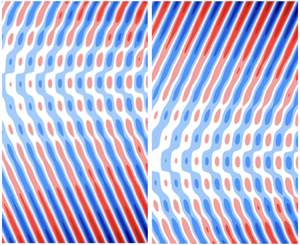
Figure 4. Spatio-temporal variation (Hovmöller diagram) of the perturbed axial velocity $u_z$ of the most unstable AMRI wave in the $(t, z)$-plane having the form of an asymmetric butterfly at $I=13$ kA (${\mathit {Ha}} \approx 101$) and $Re=1480$. In panel (a), $m=-1$ AMRI mode dominates at the bottom when the heat flux is directed from the outer to inner cylinder, while in (b) $m=1$ AMRI mode dominates at the top when the heat flux is directed from the inner to outer cylinder. This clearly shows symmetry breaking, or selection effect between the $m=\pm 1$ modes due to convection. This selection between these two modes depends on the direction of convective flow linked to the heat flux, which is consistent with the experimental findings in figure 3.

Figure 5. (a) Phase velocities and (b) normalized energy content $A^2$ (in a.u.) that is assumed to be proportional to the growth rate $\gamma _a$ of the absolute AMRI in the presence of convection at $Re=1480$. The heat flux is directed from the inner to outer cylinder. Green circles denote the experimental data, red-dashed lines correspond to the dominant $m=1$ mode, while blue lines to the subdominant $m=-1$ mode, implying symmetry breaking between these two modes in contrast to the case without convection (black dot-dashed line) where the growth rates of both $m=\pm 1$ AMRI modes are equal. Theoretical values of $A^2$ are normalized by its maximum for the dominant $m=1$ AMRI mode occurring at $Ha=116$ (corresponding to the highest growth rate $\gamma _{a,max}=0.0043$). Shaded regions are AMRI-stable.

The dynamics is significantly altered in the presence of a radial temperature gradient. The symmetry between the $m = \pm 1$ modes is broken due to convection velocity $u_{0z}$ – either of these two modes is preferred over the other depending on the direction of $u_{0z}$, as it is clearly seen in figure 4. When the heat flux is directed from the outer to inner cylinder (i.e. rising $u_{0z}>0$ near the outer cylinder and sinking $u_{0z}<0$ near the inner one), the $m =-1$ mode with ${\mathcal {I}}(k_{z,a})>0$ is dominant, that increases opposite the $z$-axis and has its phase velocity also directed opposite this axis (figure 4a). By contrast, for the reversed heat flux direction, the $m = 1$ mode with ${\mathcal {I}}(k_{z,a})<0$ is dominant, that increases along the $z$-axis and has its phase velocity also directed along this axis (figure 4b). As a result, for each direction of the heat flux, the butterfly diagram takes on a predominantly one-winged structure corresponding to the dominant mode, being mostly concentrated near the top (‘upper wing’ for $m=1$) or bottom (‘lower wing’ for $m=-1$) of the cylinder. This spatio-temporal variation of the wave velocity is in a qualitative agreement with the experimentally observed pattern of AMRI waves in figure 3.

Figure 5(a) compares the phase velocities $u$ of the AMRI waves as a function of $Ha$ from the experiments and the linear analysis in the presence of heat flux from the inner to outer cylinder. In the experiment, $u$ is measured near the outer cylinder using UDV. It is seen that the theoretical values of the phase velocities for $m=\pm 1$ AMRI-wave modes from the linear analysis match quite well with the experimental ones. This demonstrates the deviation of the phase velocity from the pure AMRI wave without convection. Due to symmetry breaking, the $m=1$ mode has somewhat larger phase velocity than the $m=-1$ mode, especially at higher $Ha$.

Figure 5(b) shows the normalized energy content $A^2$ of perturbations as obtained both from experiments and the linear stability analysis for the $m=\pm 1$ AMRI modes when the heat flux is directed from the inner to outer cylinder. The experimental data for $A^2$ represents the square of the measured r.m.s. of the axial velocity induced by AMRI, which are normalized by their maximum value with respect to $Ha$. On the other hand, the theoretical values are assumed to be proportional to the growth rate $\gamma _a$ of absolute AMRI, i.e. $A^2\propto \gamma _a$, as is typical of a slightly supercritical regime according to the Ginzburg-Landau theory of weakly nonlinear processes (e.g. Landau & Lifshitz Reference Landau and Lifshitz1987; Umurhan, Menou & Regev Reference Umurhan, Menou and Regev2007). The theoretical values of $A^2$ are also normalized by their maximum over $Ha$ corresponding to the $m=1$ AMRI mode, which is the dominant mode in this case, since its growth rate is enhanced by convection, as is seen in figure 5(b). This enhancement of the growth rate is due to the additional free energy provided selectively for the $m=1$ mode by the shear of the axial convective velocity, $u_{0z}'$. Such a normalization allows us to compare the relative magnitudes (growth rates) of the $m = \pm 1$ AMRI modes and the form of their dependence on $Ha$ in the presence and absence of convection as well as with the experimental data. Namely, the $m=1$ AMRI modes are the strongest, while the $m=-1$ AMRI modes the weakest, with the pure AMRI modes being between these two. This clearly demonstrates the nature of symmetry breaking between the $m=\pm 1$ modes caused by $u_{0z}$ – increase in the amplitude (growth rate) of one ($m=1$) mode and decrease in that of the other ($m=-1$). Note also that the critical $Ha_c\approx 62$ is lower than $Ha_c\approx 82$ for the AMRI without convection.

Thus, it is evident from figure 5 that the experimental data are in a good agreement with the theoretical results for the dominant $m=1$ AMRI mode for the radially outward heat flux both for the phase velocity and energy content, especially near the onset at $62\lesssim Ha\lesssim 100$, where the data points are closest to the $m=1$ mode curve.