


1. Introduction
Thomas (Reference Thomas2021) considered the valuation of no-negative equity guarantees (NNEG), essentially a form of long-term put option, in the presence of a lower reflecting barrier under the spot price. The pricing method was to integrate the option’s intrinsic value over a drift-neutralised density for the asset price at maturity. In Appendix B of that paper, I noted a puzzle: when the same method is applied to price a call option, the resulting pairs of call and put prices for the same strike do not satisfy the standard put-call parity. I suggested a number of pragmatic reasons why we should nevertheless adopt the price of the put for NNEG valuation, and assign some residual ambiguity to the price of the call. Similarly, in an antecedent paper, Hertrich (Reference Hertrich2015, pp. 239–240) writes that in the presence of a lower reflecting barrier “…the put price is unique and equals the risk-neutral price…the call market price can take on at least these two values, i.e. the risk-neutral call price and the imputed call price via the standard put-call parity.”
The failure of standard put-call parity hints that the barrier model allows some sort of arbitrage. Previous papers (Thomas, Reference Thomas2021; Hertrich & Zimmermann, Reference Hertrich and Zimmermann2017; Hertrich, Reference Hertrich2015; Veestraeten, Reference Veestraeten2008, Reference Veestraeten2013) all noted that the assumed instantaneous nature of reflection rules out the obvious arbitrage of buying when the spot price is exactly at the barrier, and then selling a moment later after it rises. However, this argument renders impractical only immediate arbitrage (arbitrage with no interim losses); it does not exclude arbitrage with interim losses, which requires credit to cover losses which may be incurred before an eventual gain.
Strategies of this type are indeed feasible in the barrier model. This raises economic and mathematical issues, which were not addressed in any of the previous papers just cited. Economically, it implies that the realism of the assumed price process depends on the government’s unlimited powers of intervention, and/or credit limits or other institutional features that limit scaling of the arbitrage. Mathematically, the existence of any arbitrage strategy, irrespective of its practicality of implementation, implies that no equivalent martingale measure for the asset exists; and therefore that the usual risk-neutral pricing arguments cannot be applied, at least in their standard form.
Nevertheless, delta hedging using the formulas in previous papers does exactly replicate option payoffs. The reasons are as follows. Although geometric Brownian motion (GBM) reflected at a lower barrier (“the observed price”) is not arbitrage-free, the underlying geometric Brownian motion (“the notional price”) is arbitrage-free. Furthermore, options on the observed price can be expressed as compound options on the notional price, and then expectations taken under a risk-neutral measure for the notional price. Although the notional price is not available for hedging, it turns out that for the hedging schemes we need to operate, hedging with the observed price achieves the same results as hedging with the notional price. This is because the deltas for options always tend to zero as the observed price approaches the localised irregularity at the barrier; and everywhere else, the observed price has the same standard GBM dynamics as the notional price.
The resulting replicating portfolios are martingales under the risk-neutral measure for the notional price. But the observed price is a sub-martingale under this measure, because of the interventions at the barrier (which push the observed price upwards, and are not cancelled by the removal of the drift in the standard risk-neutralisation). Similarly, the cheapest replication of a forward contract is a sub-martingale; this is because the cheapest replication of a forward contract has a static positive delta and so is positively exposed to the interventions at the barrier. These different dynamics of replicating portfolios – options martingale, forward contracts sub-martingale – inevitably mean that call, put and forward prices together will not satisfy the standard put-call parity.
Put-call parity can be restored by invoking the construct of synthetic replication for one of the options, in contrast with the more common direct replication. For a call, direct replication involves a continuously varying portfolio which is long a fraction of the underlying asset and short cash. Synthetic replication involves two elements: a long position in a forward contract and a long position in a put, both with the same strike as the call we wish to replicate. The synthetic call price is then determined as the lowest cost of replicating each of these two elements separately (via a static position for the forward and a dynamic position for the put). An analogous synthetic replication can be constructed for a put.
Under standard models for the asset price, direct replication and synthetic replication have the same costs. But in the presence of the reflecting barrier, their costs can differ. I argue that arbitrage will tend to enforce the lowest replication cost as the price for any derivative (I call this “the principle of the lowest price,” in contrast to the usual “law of one price”). For a put, direct replication always has a lower initial cost, and never produces interim losses. So direct replication is unambiguously the best way of replicating a put. For a call, synthetic replication always has a lower initial cost, but it produces interim losses. So the preferred replication strategy (and hence price) of a call depends on what margin payments need to be made on these losses.
If the price of a call is ambiguous, then put-call parity is also in general ambiguous. But we can define it if we assume that no margin payments are required on interim losses. In that case, synthetic replication becomes unambiguously preferable for a call, so put-call parity then takes the form Synthetic Call price – Put price = Forward Contract price.
Earlier work on option pricing in the presence of a lower reflecting barrier includes the following papers. For calls with a lower barrier, Veestraeten (Reference Veestraeten2008) derived the direct replication price, and Veestraeten (Reference Veestraeten2013) considered a combination of upper and lower barriers to represent a foreign exchange currency band. For puts with a lower barrier, Hertrich & Veestraeten (Reference Hertrich and Veestraeten2013) stated the result, and Hertrich (Reference Hertrich2015) and Hertrich & Zimmermann (Reference Hertrich and Zimmermann2017) gave a full derivation. Thomas (Reference Thomas2021) suggested an application to the valuation of no-negative-equity guarantees on equity release mortgages. Each of these papers focused mainly either on call options (Veestraeten, Reference Veestraeten2008, Reference Veestraeten2013) or on put options (Hertrich, Reference Hertrich2015; Hertrich & Zimmermann, Reference Hertrich and Zimmermann2017; Thomas, Reference Thomas2021), but not both; this may explain why the complications highlighted in the present paper have not previously been considered. In earlier actuarial literature, Gerber & Pafumi (Reference Gerber and Pafumi2000) and Imai & Boyle (Reference Imai and Boyle2001) considered the related problem of pricing of a dynamic guarantee on an investment fund, where the guarantee is modelled as a reflecting barrier under the fund price. Ko et al. (Reference Ko, Shiu and Wei2010) considered an investment fund with two reflecting barriers, representing a lower guarantee plus withdrawals to prevent the fund from exceeding an upper limit. The formulas for these related problems can be reconciled with those in this paper, see e.g. Appendix D of Thomas (Reference Thomas2021). Buckner et al. (Reference Buckner, Dowd and Hulley2022) draw attention to the arbitrage opportunities created by a reflecting barrier; I agree with this observation, but not with the inference that the option formulas have no justification.
The conclusions of this paper can be compared with those in the literature on option prices in the presence of a bubble in the price of the underlying asset (e.g. Cox & Hobson, Reference Cox and Hobson2005; Heston et al. Reference Heston, Loewenstein and Willard2007; Jarrow et al., Reference Jarrow, Protter and Shimbo2007; Protter, Reference Protter, Henderson and Sircar2013). In both settings, the standard put-call parity fails to hold. In a bubble, the current asset price exceeds its discounted expectation under the pricing measure at a future date; but with a lower reflecting barrier, this inequality is reversed. Protter (Reference Protter, Henderson and Sircar2013) distinguishes between “fundamental” and “market” prices for options in the presence of a bubble, where the fundamental price is the discounted expectation under the risk-neutral measure. For a put, market and fundamental prices in a bubble are the same (as in the barrier model); but for a call, market and fundamental prices differ by an amount equivalent to the difference Synthetic Call – Call in this paper (Protter, Reference Protter, Henderson and Sircar2013, Equation (80)). His difference has the opposite sign to ours: in a bubble, the current market price of the asset (or a call on the asset) exceeds its discounted expectation under the pricing measure, but with a lower reflecting barrier, the inequality is reversed.
The rest of this paper is organised as follows. Section 2 gives the set-up of the barrier model and the derivation of option prices and deltas, and reports simulations showing satisfactory convergence of pricing errors and replication errors. Section 3 considers put-call parity, and hence direct and synthetic replication; it concludes that a put should always be priced by direct replication, but the price of a call is ambiguous. Application of the points made in section 3 is illustrated in section 4 for a put, and section 5 for a call. Section 6 considers the arbitrage possibilities in the barrier model, and their susceptibility to credit limits and other institutional constraints. Section 7 gives further discussion, and section 8 states conclusions.
2. The Barrier Model
2.1. Concept
The barrier is a metaphor for policymaker actions, such as interventions to support prices after a large fall in the housing market (Thomas, Reference Thomas2021, section 2), or central bank currency purchases supporting a floor under an exchange rate (Hertrich, Reference Hertrich2015; Hertrich & Zimmermann, Reference Hertrich and Zimmermann2017). Alternatively, the barrier represents the different economic properties of underlying assets such as freehold land (an absolute claim), compared with the underlying assets such as equity (a residual claim) as in many other option valuations (Thomas, Reference Thomas2021, section 3).
We start with a standard geometric Brownian motion for the price process. We then impose a reflecting barrier somewhere below the lower of the spot price and the strike price (i.e. b < min (S, K)). The strike can be either lower or higher than the spot price, i.e. in or out of the money. If the spot price hits the barrier, reflection occurs instantaneously and with infinitesimal size. We can think of this as the State making a small purchase, just sufficient to prevent the price falling below the barrier. The instantaneous nature of the reflection means that the price does not spend any finite time at the barrier, so the obvious arbitrage of buying when the price is exactly at the barrier is not practically feasible (but there will be more to say about arbitrage later).
2.2. Derivations
The derivations make use of two price processes: a process for the observed price S t in a world with a reflecting barrier; and a process for the notional price N t of an asset with the same starting value today and same instantaneous dynamics, but in a world without a barrier.
We assume that the notional price N t is a geometric Brownian motion, specified as usual by
 \begin{align} \textrm{d} {N_t} = \left( {\mu - q} \right)\!{N_t}\textrm{d} t + \sigma {N_t}\;{\rm{d}}{W_t}\end{align}
where μ is the real-world expected total return on the asset, q is the yield (assumed to be continuous), σ is the diffusion, and dW t is the increment of a standard Wiener process. The solution of this is
 \begin{align} {N_t} = {N_0}\exp \!\left\{ {\left( {\mu - {{q - {\sigma ^2}} \big/ 2}} \right)\!t + \sigma \!{W_t}} \right\}\end{align}
where N 0 is the notional price today.
Now consider a lower reflecting barrier at price level b. Because of the barrier, the observed price process S t will be
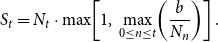 \begin{align} {S_t} = {N_t} \cdot \max\! \left[ {1,\;\mathop {\max }\limits_{0 \le n \le t} \!\left( {\frac{b}{{{N_n}}}} \right)} \right].\end{align}
In words: the process S t is equal to N t , if N t has never gone below the barrier; or an up-rated version of N t which “undoes” the maximum proportional deficit relative to the barrier, if it has. Figure 1 shows how it works, for one unfavourable simulation over 25 years.
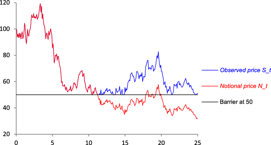
Figure 1. One simulation for the prices N t and S t .
Now transform to an arithmetic Brownian motion: divide Equation (3) by b (so that the barrier becomes 1) and then take logs (so that the barrier becomes zero)Footnote 1 . This gives:
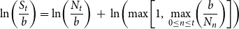 \begin{align} \ln\! \left( {\frac{{{S_t}}}{b}} \right) = \ln\! \left( {\frac{{{N_t}}}{b}} \right)\; + \;\ln\! \left( {\max\! \left[ {1,\;\mathop {\max }\limits_{0 \le n \le t} \!\left( {\frac{b}{{{N_n}}}} \right)} \right]} \right)\end{align}
or, writing Z t = ln(S t /b), Y t = ln(N t /b), and noting ln(max(a,b)) = max(ln a, ln b), and N n = b exp Y n :
 \begin{align} {Z_t} = {Y_t} + \max\! \left[ {0,\;\mathop {\max }\limits_{0 \le n \le t} \!\left( { - {Y_n}} \right)} \right]\end{align}
or
 \begin{align} {Z_t} = {Y_t} + {L_t}.\end{align}
Figure 2, which is the same simulation as in Figure 1 but with the transformation just given, shows how it works. Note that the blue line Z t is obtained by taking the red line Y t and then adding L t , the running maximum shortfall of Y t below zero. L t is a non-decreasing continuous process, which increases whenever Z t touches the barrier. This construction ensures that Z t never spends any finite time at the barrier, and there are no jumps. L t can also be thought of as the total quantum of the interventions at the barrier between time 0 and time t; this quantum is finite, despite the individual interventions being infinitesimalFootnote 2 .
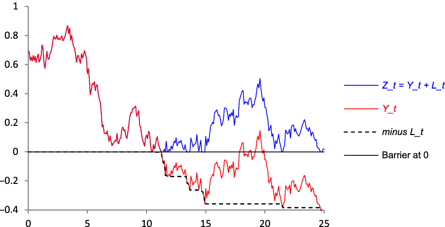
Figure 2. One simulation for the log prices Y t and Z t .
Now note that Y t is an arithmetic Brownian motion, for which Ito’s lemma gives
 \begin{align} \textrm{d}{Y_t} = {\rm{d}}\ln \!\left( {{{{N_t}} \big/ b}} \right) = {\rm{d}}\ln {N_t} = \left( {\mu - q - {{{\sigma ^2}} \big/ 2}} \right)\!{\rm{d}}t + \sigma {\rm{d}}{W_t}\end{align}
Then, note that Z
t
is a semi-martingale, because it can be decomposed into a martingale (the W
t
term) and two finite variation processes, the drift and the reflection. So we can also apply Ito’s lemma to ${Z_t} = f\!\left( {t,W,L} \right).$
This gives
${Z_t} = f\!\left( {t,W,L} \right).$
This gives
 \begin{align} {\rm{d}} {Z_t} = {\rm{d}}\ln\! \left( {{{{S_t}} \big/ b}} \right) = {\rm{d}}\ln\! \,{S_t} = \left( {\mu - {{q - {\sigma ^2}} \big/ 2}} \right)\!{\rm{d}} t + \sigma {\rm{d}}{W_t} + {\rm{d}} {L_t}\end{align}
which is the same as Equation (7), plus ${\rm{d}} {L_t}$
, and second-order terms involving
${\rm{d}} {L_t}$
, and second-order terms involving ${\rm{d}} L {\rm{d}}W,$ ${\rm{d}} L {\rm{d}} t,$
and
${\rm{d}} L {\rm{d}} t,$
and ${\rm{d}} L {\rm{d}} L$
which are all zero (because of the infinitesimal size of the increments at reflection).
${\rm{d}} L {\rm{d}} L$
which are all zero (because of the infinitesimal size of the increments at reflection).
Comparing Equations (7) and (8), we see that reflected Brownian motion Z
t
has the same stochastic process as the ordinary Brownian motion Y
t
, except for the extra ${\rm{d}} {L_t}$
term. This term is zero at all times, except when Z
t
touches the barrier (equivalently: Y
t
makes a new low below zero), where it generates an infinitesimal increment.
${\rm{d}} {L_t}$
term. This term is zero at all times, except when Z
t
touches the barrier (equivalently: Y
t
makes a new low below zero), where it generates an infinitesimal increment.
The equivalent equations for the non-logged variables are
 \begin{align} \textrm{d} {N_t} = \left( {\mu - q} \right){N_t}\textrm{d} t + \sigma {N_t}\;{\rm{d}} {W_t}\end{align}
and
 \begin{align} \textrm{d} {S_t} = \left( {\mu - q} \right)\!{S_t}\textrm{d} t + \sigma {S_t}\;{\rm{d}} {W_t} + {\rm{d}} {L_t}.\end{align}
By replacing the expected total return μ in Equation (9) with the risk-free rate r, we get a process for N
t
for a new measure $\mathbb{Q}$
N
, under which the geometric Brownian motion N
t
discounted at r – q is a martingale:
$\mathbb{Q}$
N
, under which the geometric Brownian motion N
t
discounted at r – q is a martingale:
 \begin{align} \textrm{d} {N_t} = \left( {r - q} \right){N_t}\textrm{d} t + \sigma {N_t}\;{\rm{d}} W_t^{{\mathbb{Q}_N}}\end{align}
where $W_t^{{\mathbb{Q}_N}}$
is a Wiener process under the new measure
$W_t^{{\mathbb{Q}_N}}$
is a Wiener process under the new measure $\mathbb{Q}$
N
Footnote
3
.
$\mathbb{Q}$
N
Footnote
3
.
Earlier papers (Thomas, Reference Thomas2021; Hertrich & Zimmermann, Reference Hertrich and Zimmermann2017; Hertrich, Reference Hertrich2015; Veestraeten Reference Veestraeten2008, Reference Veestraeten2013) implicitly proceeded on the basis that this change of measure also turned the discounted observed price S
t
into a martingale. But this is not correct, because of the ${\rm{d}} {L_{t.}}$
term in Equation (10). The discounted notional price (red line in Figure 1) is a martingale under
${\rm{d}} {L_{t.}}$
term in Equation (10). The discounted notional price (red line in Figure 1) is a martingale under $\mathbb{Q}$
N
(i.e.
$\mathbb{Q}$
N
(i.e. ${e^{ - \left( {r - q} \right)T}}{{\rm{E}}_{{Q_N}}}[{N_T}] = {S_0}$
), but the discounted observed price (blue line) tends to be pushed upwards at the barrier, and so is a sub-martingale under
${e^{ - \left( {r - q} \right)T}}{{\rm{E}}_{{Q_N}}}[{N_T}] = {S_0}$
), but the discounted observed price (blue line) tends to be pushed upwards at the barrier, and so is a sub-martingale under $\mathbb{Q}$
N
(i.e.
$\mathbb{Q}$
N
(i.e. ${e^{ - \left( {r - q} \right)T}}{{\rm{E}}_{{Q_N}}}[{S_T}] \geq {S_0}$
).
${e^{ - \left( {r - q} \right)T}}{{\rm{E}}_{{Q_N}}}[{S_T}] \geq {S_0}$
).
The earlier papers obtained pricing formulas for options on S
t
as discounted $\mathbb{Q}$
N
-expectations of terminal payoffs. The usual justification is that because the Black-Scholes partial differential equation for the price of an option does not depend directly on investor preferences, its solution must be consistent with the expected value of the option in a world of risk-neutral preferences. In the Black-Scholes model, we represent risk-neutral preferences by setting the expected total return on the asset to be the same as the risk-free rate r, or stated differently, changing the measure to make the stochastic process for the discounted asset price a martingale. But in the presence of the barrier, we have already noted that discounted S
t
is not a martingale under
$\mathbb{Q}$
N
-expectations of terminal payoffs. The usual justification is that because the Black-Scholes partial differential equation for the price of an option does not depend directly on investor preferences, its solution must be consistent with the expected value of the option in a world of risk-neutral preferences. In the Black-Scholes model, we represent risk-neutral preferences by setting the expected total return on the asset to be the same as the risk-free rate r, or stated differently, changing the measure to make the stochastic process for the discounted asset price a martingale. But in the presence of the barrier, we have already noted that discounted S
t
is not a martingale under $\mathbb{Q}$
N
(see previous paragraph). Furthermore, because of the interventions at the barrier, there is no change of drift that can make it so, and hence, the usual procedure does not work. Nevertheless, it turns out that
$\mathbb{Q}$
N
(see previous paragraph). Furthermore, because of the interventions at the barrier, there is no change of drift that can make it so, and hence, the usual procedure does not work. Nevertheless, it turns out that $\mathbb{Q}$
N
-expectations do give hedging schemes which exactly replicate option payoffs, albeit for subtly different reasons from the usual argument. These reasons will be explained in section 2.4 below; but first, I state the
$\mathbb{Q}$
N
-expectations do give hedging schemes which exactly replicate option payoffs, albeit for subtly different reasons from the usual argument. These reasons will be explained in section 2.4 below; but first, I state the $\mathbb{Q}$
N
-expectations and the corresponding deltas as in Thomas (Reference Thomas2021).
$\mathbb{Q}$
N
-expectations and the corresponding deltas as in Thomas (Reference Thomas2021).
For a call, the $\mathbb{Q}$
N
-expectation gives a price of
$\mathbb{Q}$
N
-expectation gives a price of
 \begin{align} {C_B} = {{\rm{e}}^{ - rT}}{{\rm{E}}_{{\mathbb{Q}_N}}}{\left[ {{S_T} - K} \right]^ + } = \;{e^{ - rT}}\int_K^\infty {\left( {{S_T} - K} \right)} \,f({S_T})\;{\rm{d}}{S_T}\end{align}
where the B-subscript on ${C_B}$
denotes that this is a call in the presence of a lower reflecting barrier. Conveniently, an expression is available for the density of Z
t
as a function of Y
t
, and hence also the re-transformed density for S
t
= b exp Z
t
, the observed priceFootnote
4
. This enables us to evaluate the integral as follows (for a full derivation, see Veestraeten, Reference Veestraeten2008):
${C_B}$
denotes that this is a call in the presence of a lower reflecting barrier. Conveniently, an expression is available for the density of Z
t
as a function of Y
t
, and hence also the re-transformed density for S
t
= b exp Z
t
, the observed priceFootnote
4
. This enables us to evaluate the integral as follows (for a full derivation, see Veestraeten, Reference Veestraeten2008):
 \begin{align} \begin{array}{l}{C_B} = S {e^{ - qT}}\,\Phi\!\left( {{z_1}} \right) - K {e^{ - rT}}\Phi\!\left( {{z_1} - \sigma \sqrt T } \right)\\[5pt] \quad \quad \quad + \dfrac{1}{\theta }\left\{ \begin{array}{l} S {e^{ - qT}}\,{\left( {\dfrac{b}{S}} \right)^{1 + \theta }}\Phi\!\left( {{z_2}} \right)\\[12pt] - K {e^{ - rT}}{\left( {\dfrac{b}{K}} \right)^{1 - \theta }}\Phi\!\left( {{z_2} - \theta \sigma \sqrt T } \right)\end{array} \right\}\end{array}\end{align}
with K= strike price, S = current spot priceFootnote 5 , T = term of the option, b = barrier price, r = risk-free rate, q = asset yield (“deferment rate,” in the NNEG context), σ = volatility, Φ(.) is the standard Normal cumulative distribution function, and
 \begin{align*} {z_1} = \frac{1}{{\sigma \sqrt T }}\left[ {\ln\! \left( {\frac{S}{K}} \right) + \left( {r - q + \frac{{{\sigma ^2}}}{2}} \right)T} \right],\,{z_2} = \frac{1}{{\sigma \sqrt T }}\left[ {\ln\! \left( {\frac{{{b^2}}}{{KS}}} \right) + \left( {r - q + \frac{{{\sigma ^2}}}{2}} \right)T} \right],\end{align*} $\quad \theta = 2\dfrac{{\left( {r - q} \right)}}{{{\sigma ^2}}}\;\;$
with r ≠ q.Footnote
6
$\quad \theta = 2\dfrac{{\left( {r - q} \right)}}{{{\sigma ^2}}}\;\;$
with r ≠ q.Footnote
6
We can make the following observations on Equation (13).
-
(i) The first line is the Black-Scholes formulaFootnote 7 for a call, and then there is the 1/θ term (say Call Adjustment). The Call Adjustment evaluates as positive, but reduces to 0 for b = 0, as expected.
-
(ii) The definition of S t in Equation (3) excludes the possibility of S t having touched the barrier in the past, i.e. before the time designated as zero. To be consistent with this set-up, we should always define time 0 as the current time when we do an option valuation, and define the initial notional price as the current price (i.e. N 0 = S 0). The density underlying Equation (13) assumes this, i.e. it does not incorporate the possibility of an uprating effect on S t from past barrier touches, which would require extra terms.
-
(iii) Some care is needed with the volatility parameter σ. From Equation (1), we can see that σ is the annualised standard deviation of the logarithmic price change of the notional price N t (i.e. the GBM volatility in the absence of the reflecting barrier). We can estimate σ by observing the standard deviation of short-term changes in the observed log price, $\ln\! \left( {{{{S_t}} \big/ {{S_{t - 1}}}}} \right)$
, over a period in which the barrier has not been touched, and then applying the usual
$\sqrt t $
-scaling to give an annualised value. But we cannot apply
$\sqrt t $
-scaling to σ to give the standard deviation of
$\ln\! \left( {{{{S_T}} \big/ {{S_0}}}} \right)$
over a long period T, because this will be reduced by the presence of the barrier. The usual
$\sqrt t $
-scaling is predicated on geometric Brownian motion, but that is not what we have in the observed priceFootnote
8
.
$\ln\! \left( {{{{S_t}} \big/ {{S_{t - 1}}}}} \right)$
, over a period in which the barrier has not been touched, and then applying the usual
$\sqrt t $
-scaling to give an annualised value. But we cannot apply
$\sqrt t $
-scaling to σ to give the standard deviation of
$\ln\! \left( {{{{S_T}} \big/ {{S_0}}}} \right)$
over a long period T, because this will be reduced by the presence of the barrier. The usual
$\sqrt t $
-scaling is predicated on geometric Brownian motion, but that is not what we have in the observed priceFootnote
8
.


Similarly, for a put, the $\mathbb{Q}$
N
-expectation gives a price of
$\mathbb{Q}$
N
-expectation gives a price of
 \begin{align} {P_B} = {{\rm{e}}^{ - rT}}{{\rm{E}}_{{\mathbb{Q}_N}}}{\left[ {K - {S_T}} \right]^ + } = \;{e^{ - rT}}\int_b^K {\left( {K - {S_T}} \right)} \,f({S_T})\;{\rm{d}}{S_T}\end{align}
which evaluates as
 \begin{align} \begin{array}{l}\quad {P_B} = K {e^{ - rT}}\Phi\!\left( { - {z_1} + \sigma \sqrt T } \right) - S{e^{ - qT}}\,\Phi\!\left( { - {z_1}} \right)\\[5pt] \quad \quad \quad\;- b{{\mathop{\rm e}\nolimits} ^{ - rT}}\Phi\!\left( { - {z_3} + \sigma \sqrt T } \right) + S{e^{ - qT}}\,\Phi\!\left( { - {z_3}} \right)\\[5pt] \quad \quad \quad \; + \dfrac{1}{\theta }\left\{ \begin{array}{l}b{e^{ - rT}}\Phi\!\left( { - {z_3} + \sigma \sqrt T } \right)\\[5pt] - S {e^{ - qT}}\,{\left( {\dfrac{b}{S}} \right)^{1 + \theta }}\left[ {\Phi\!\left( {{z_4}} \right) - \Phi\!\left( {{z_2}} \right)} \right]\\[12pt] - K {e^{ - rT}}{\left( {\dfrac{b}{K}} \right)^{1 - \theta }}\Phi\!\left( {{z_2} - \theta \sigma \sqrt T } \right)\end{array} \right\}\end{array}\end{align}
with
 \begin{align*} {z_3} = \frac{1}{{\sigma \sqrt T }}\left[ {\ln\! \left( {\frac{S}{b}} \right) + \left( {r - q + \frac{{{\sigma ^2}}}{2}} \right)T} \right],\,{z_4} = \frac{1}{{\sigma \sqrt T }}\left[ {\ln\! \left( {\frac{b}{S}} \right) + \left( {r - q + \frac{{{\sigma ^2}}}{2}} \right)T} \right].\end{align*}
For a full derivation, see Hertrich & Zimmermann (Reference Hertrich and Zimmermann2017), supported by Appendices A to C of Hertrich & Zimmermann (Reference Hertrich and Zimmermann2014).
The delta for a call is found by differentiating Equation (13) with respect to the price of the underlying asset:
 \begin{align} \quad \quad \quad {\delta _{{C_B}}} = \frac{{\partial {C_B}}}{{\partial S}} = {e^{ - qT}}\left\{ {\Phi\!\left( {{z_1}} \right) - {{\left( {\frac{b}{S}} \right)}^{1 + \theta }}\Phi\!\left( {{z_2}} \right)} \right\}.\end{align}
Similarly, the delta for a put is:
 \begin{align} \quad \quad \quad {\delta _{{P_B}}} = \;\frac{{\partial {P_B}}}{{\partial S}} = {e^{ - qT}}\left\{ {\Phi\!\left( {{z_1}} \right) - \Phi\!\left( {{z_3}} \right) + {{\left( {\frac{b}{S}} \right)}^{1 + \theta }}\left[ {\Phi\!\left( {{z_4}} \right) - \Phi\!\left( {{z_2}} \right)} \right]} \right\}.\end{align}
Derivations of Equations (16) and (17) are given in Appendix A (Supplementary Material).
2.3. Simulation
We now specify some example parameters which will be used where appropriate throughout the rest of the paper: let spot price S = 1, barrier b = 0.5, strike K = 1 (i.e. at-the-money), risk-free rate r = 0.015, asset yield q = 0.01, volatility σ = 13%, and term T = 25 years. These parameters are intended to be representative of the NNEG context as in Thomas (Reference Thomas2021).
Simulation is useful for two distinct purposes: to verify that the formulas are correct $\mathbb{Q}$
N
-expectations, and to show that delta hedging based on these formulas exactly replicates option payoffs.
$\mathbb{Q}$
N
-expectations, and to show that delta hedging based on these formulas exactly replicates option payoffs.
For the first purpose, we simulate the asset price using Equations (2) and (3), but with the drift μ replaced by r, a fixed large number of time steps, and then vary the number of simulations. We measure pricing error as mean discounted option payoff less the analytical option formula. This is illustrated for a put in Figure 3, a log-log plot of confidence intervals for the pricing error against the number of simulations N
s
. The slope of −0.5 shows that the Monte Carlo means converge on the analytical formulas in line with ${{1\,} / {\sqrt {{N_S}} }}.$
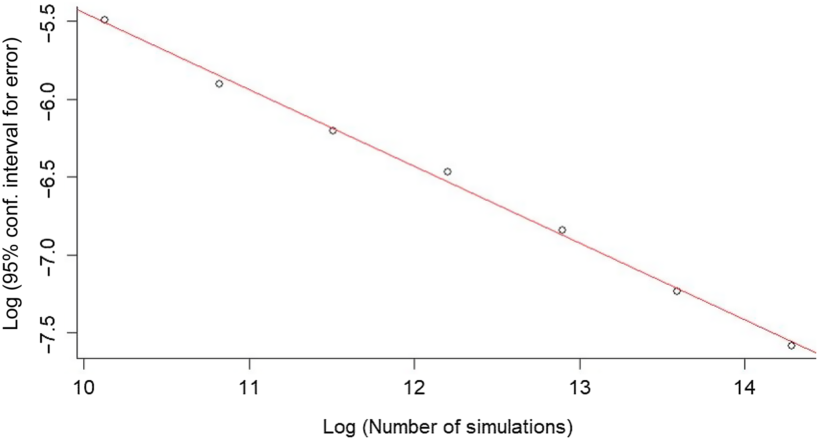
Figure 3. Convergence of put pricing errors to zero with increasing number of simulations.
For the second purpose, we again simulate the asset price using Equations (2) and (3), but with a real-world drift μ = 0.03 (say), a fixed number of simulations, and then vary the number of time steps. We find that replication schemes based on initial wealth as per the call and put formulas in Equations (13) and (15), and deltas as in Equations (16) and (17), exactly replicate option payoffs, for any simulated real-world drift of the asset price. This is illustrated for a put in a Figure 4, a log-log plot of standard deviations of replication errors against the number of time steps N
T
. The slope of −0.5 shows that the replication errors converge in line with ${{1\,} \big/ {\sqrt {{N_T}} }}.$
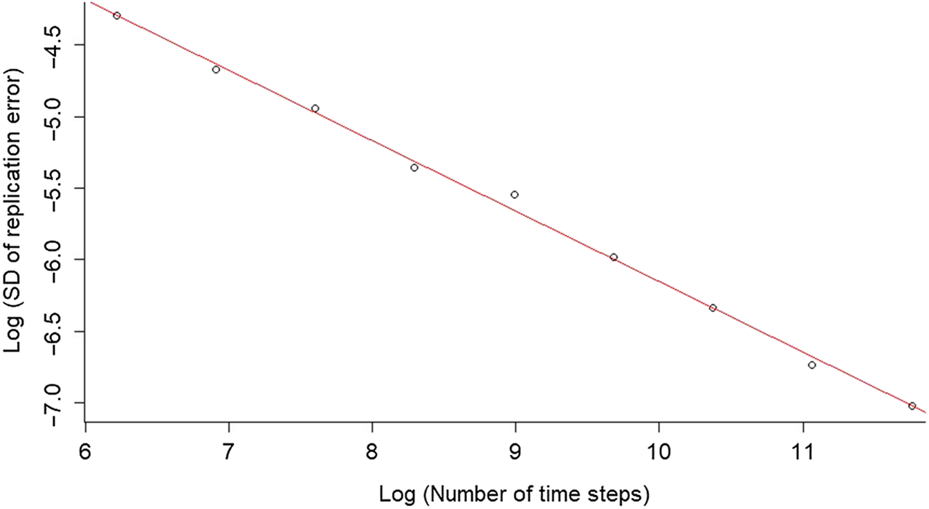
Figure 4. Convergence of put replication errors to zero with increasing number of time steps.
2.4. Why delta hedging exactly replicates option payoffs
Section 2.2 noted that because of the irregularity at the barrier, the observed price S
t
is not a martingale under $\mathbb{Q}$
N
, and so part of the standard justification for risk-neutral pricing does not apply to options on S
t
. To understand why option replication by hedging schemes based on
$\mathbb{Q}$
N
, and so part of the standard justification for risk-neutral pricing does not apply to options on S
t
. To understand why option replication by hedging schemes based on $\mathbb{Q}$
N
-expectations still works, first recall that the observed price S
t
is a function of the notional price N
t
. Specifically, the definition of S
t
in Equation (3) can be written as
$\mathbb{Q}$
N
-expectations still works, first recall that the observed price S
t
is a function of the notional price N
t
. Specifically, the definition of S
t
in Equation (3) can be written as
 \begin{align} {S_t} = {N_t} \cdot \max\! \left( {1,\;\mathop {\max }\limits_{0 \le n \le t} \!\left( {\frac{b}{{{N_n}}}} \right)} \right)\;\; = {N_t}.\exp \!\left\{ {\;{\rm{max}}\!\left[ {0,\ln b - \ln\! \mathop {\min }\limits_{0 \le n \le t} {N_n}} \right]\;} \right\}\end{align}
where the max[.] term on the right is a lookback put (with fixed strike ln b) on the log-minimum of N. So a put on S T can be expressed as a compound option on N T , with payoff of
 \begin{align} {\rm{max}}\!\left( {K - {S_T},0} \right) = \max\! \left( {\;K - {N_T}.\exp \!\left\{ {\;{\rm{max}}\!\left[ {0,\ln b - \ln\! \mathop {\min }\limits_{0 \le n \le T} {N_n}} \right]\;} \right\},0\;} \right)\end{align}
or in words, a put on S
T
is a put on: N
T
times the exponential of a logarithmic lookback put on the minimum of N
Footnote
9
. As for any derivative of N
T
, the discounted $\mathbb{Q}$
N
-expectation of this payoff is a risk-neutral price with reference to N
t
, and if N
t
were available for hedging, we could replicate its payoff by hedging against N
t
using a delta
$\mathbb{Q}$
N
-expectation of this payoff is a risk-neutral price with reference to N
t
, and if N
t
were available for hedging, we could replicate its payoff by hedging against N
t
using a delta ${{\partial {P_t}} \big/ {\partial {N_t}}}$
, where P
t
is the put price at time t. Then, note the following points:
${{\partial {P_t}} \big/ {\partial {N_t}}}$
, where P
t
is the put price at time t. Then, note the following points:
-
(i) By inspection of Equation (18):
-
(a) When N t is not at a new minimum below b, then S t is just a piecewise scaling of N t . Specifically, Equation (18) says
${S_t} = {N_t}{\tilde p_t}$
, where
${\tilde p_t}$
is the exponentiated payoff at time t of the logarithmic lookback put. The scaling factor,
${\tilde p_t} = {{\partial {S_t}} \big/ {\partial {N_t}}}$
for all S
t
≠ b, is constant throughout each interval when N
t
is not at a new minimum below b, corresponding to flat segments of the dashed line in Figure 2. -
(b) When N t hits a new minimum below b, substituting ln N t for
$\ln\! \mathop {\min }\limits_{0 \le n \le t} {N_n}$
in Equation (18) gives
${S_t} = {N_t}\!\left( {{b \big/ {{N_t}}}} \right) = b$
. In other words: whenever N
t
hits a new minimum below b (equivalently: S
t
touches the barrier), the dependence of S
t
on N
t
vanishes. So the derivative
${{\partial {S_t}} \big/ {\partial {N_t}}}$
must also vanish.
-
-
(ii) By the chain rule,
${{{\partial {P_t}} \big/ {\partial S}}_t} = {{\partial {P_t}} \big/ {\partial {N_t} \times {{{{\partial {N_t}} \big/ {\partial S}}}_t}}}$
(where P
t
is the call price evaluated at time t). So the option deltas with respect to S
t
and N
t
are related in the same way as in (i), but with the inverse scaling
${1 \big/ {\,{{\tilde p}_t}}}$
, and both must vanish when S
t
touches the barrier. -
(iii) Hence for the compound option in Equation (19), hedging with N t using a delta
${{\partial {P_t}} \big/ {\partial {N_t}}}$
(which we cannot do) gives the same results as hedging with S
t
using a delta
${{\partial {P_t}} \big/ {\partial {S_t}}}$
(which we can do). -
(iv) By inspection of Equation (17),
${{\partial {P_B}} \big/ {\partial {S_t}}} \to 0$
as
$S \to b$
, as expected from the “vanishing derivative” argument above. The same is true of
${{\partial {C_B}} \big/ {\partial {S_t}}}$
in Equation (16).


A further intuition for the vanishing derivatives is as follows. When N
t
(a geometric Brownian motion) is near its current lookback minimum, ${\tilde p_t}$
, it will almost surely go further below this before time T, thus establishing a new minimum. So infinitesimal changes in
${\tilde p_t}$
, it will almost surely go further below this before time T, thus establishing a new minimum. So infinitesimal changes in ${\tilde p_t}$
(and hence S
t
) at the current time will have no effect on the terminal value
${\tilde p_t}$
(and hence S
t
) at the current time will have no effect on the terminal value ${\tilde p_T}$
(and hence also, the terminal value S
T
). For a rigorous proof see the paper on lookback options by Goldman et al. (Reference Goldman, Sosin and Gatto1979).
${\tilde p_T}$
(and hence also, the terminal value S
T
). For a rigorous proof see the paper on lookback options by Goldman et al. (Reference Goldman, Sosin and Gatto1979).
Another way to look at this is via the stochastic process representations of N
t
and S
t
in Equations (9) and (10). Notice that when S
t
is above the barrier, it is just a scaled version of N
t
, with the same GBM dynamics. When S
t
touches the barrier, its dynamics deviate from those of N
t
, because of the ${\rm{d}} {L_t}$
reflection term; but at this point, the option delta goes smoothly to zero, so our replicating portfolio has no exposure to the
${\rm{d}} {L_t}$
reflection term; but at this point, the option delta goes smoothly to zero, so our replicating portfolio has no exposure to the ${\rm{d}} {L_t}$
term. Stated differently, under the measure
${\rm{d}} {L_t}$
term. Stated differently, under the measure $\mathbb{Q}$
N
, the discounted option replicating portfolios based on delta hedging using S
t
are martingales; but S
t
itself is a sub-martingale, because of the
$\mathbb{Q}$
N
, the discounted option replicating portfolios based on delta hedging using S
t
are martingales; but S
t
itself is a sub-martingale, because of the ${\rm{d}} {L_t}$
term.
${\rm{d}} {L_t}$
term.
The above arguments explain why hedging using deltas derived from $\mathbb{Q}$
N
-expectations successfully replicates option payoffs, despite the fact that S
t
is not a martingale under
$\mathbb{Q}$
N
-expectations successfully replicates option payoffs, despite the fact that S
t
is not a martingale under $\mathbb{Q}$
N
. But the difference in dynamics between replicating portfolios (martingales) and asset price (sub-martingale) under
$\mathbb{Q}$
N
. But the difference in dynamics between replicating portfolios (martingales) and asset price (sub-martingale) under $\mathbb{Q}$
N
hints at complications with put-call parity, which we examine next.
$\mathbb{Q}$
N
hints at complications with put-call parity, which we examine next.
3. Put-Call Parity
3.1. Intuition: calls are inefficient, puts efficient
We start with a graphical intuition that foreshadows much of what follows. Briefly, a call is an “inefficient” contract in the sense that its payoff may fail to give credit for the full effect of any interventions when the asset touches the barrier along the asset path to that payoff. A put does not have this feature, and so is “efficient.”
To see this, look at Figure 5. Each panel shows one sample path for the notional price N
t
(red), and the corresponding observed price S
t
(blue). Notice that in the left panel, the payoff of a call, $\max\! \left( {{S_T} - K,0} \right)$
, is less than the accumulated effect (S
T
– N
T
) of the interventions (or equivalently, the reflection) along the asset path. In contrast, in the right panel, the payoff of a put,
$\max\! \left( {{S_T} - K,0} \right)$
, is less than the accumulated effect (S
T
– N
T
) of the interventions (or equivalently, the reflection) along the asset path. In contrast, in the right panel, the payoff of a put, $\max\! \left( {K - {S_T},0} \right)$
, is reduced by the full accumulated effect (S
T
– N
T
) of the interventions, compared with the much larger payoff if there were no barrier (i.e. if the red line represented the observed price).
$\max\! \left( {K - {S_T},0} \right)$
, is reduced by the full accumulated effect (S
T
– N
T
) of the interventions, compared with the much larger payoff if there were no barrier (i.e. if the red line represented the observed price).
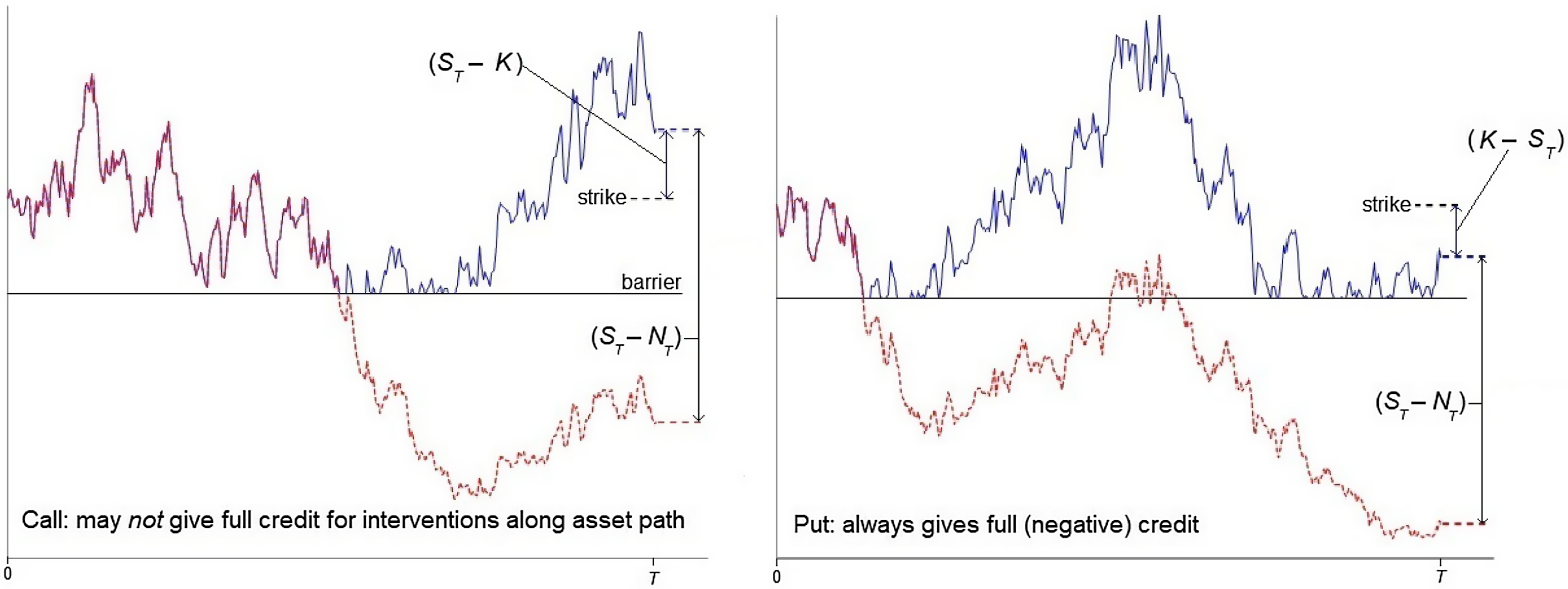
Figure 5. Calls are inefficient, puts efficient.
It is possible to draw paths where a call payoff includes the full effect of any interventions, and a put payoff includes none: the red line in each panel just needs to terminate above the strike. But for such paths, the put payoff is zero anyway (both before and after the interventions), so such paths are inconsequential for the valuation of a put. In general, whenever an option has a positive terminal payoff:
-
(i) a call payoff does not always include the full positive effect (left panel in Figure 5); but
-
(ii) a put payoff always does always include the full negative effect (right panel in Figure 5)
of any interventions along the path to that payoff.
Observations (i) and (ii) suggest that the barrier has, in some sense, a more fundamental effect on a put than on a call.
Also note that:
-
(a) for a call, the barrier redistributes the density of payoffs compared to that which prevails with no barrier, but without changing its support
$\left[ {0,\infty } \right]$
;but
-
(b) for a put, the barrier both redistributes the density of payoffs, and narrows its support from [0, K] to [0, K – b].

Observations (a) and (b) again suggest that the barrier has a more fundamental effect on a put than on a call.
Now recall that by parity, call and put payoffs are mutually redundant: if we have one plus the forward contract, we can always synthesise the payoff of the other. So rather than directly replicating a call, it might be cheaper to synthesise its payoff as a forward plus a put.
3.2. Definition of put-call parity
Instead of the usual general reasoning about payoffs, it is useful for our present purposes to derive put-call parity by explicitly differencing call and put prices:
 \begin{align} {\rm{Call\; price}} - {\rm{Put}}\,{\rm{price}} = {\rm{Forward\; Contract\; price}}\end{align}
In the Black-Scholes model appropriate for the notional price N t (a geometric Brownian motion), if the Black-Scholes call and put prices are C and P (assuming the same strike K as the forward contract), we have
 \begin{align} C - P = \left[ {N{e^{ - qT}}\Phi\!\left( {{z_1}} \right) - K{e^{ - rT}}\Phi\!\left( {{z_1} - \sigma \sqrt T } \right)} \right] - \left[ {K{e^{ - rT}}\Phi\!\left( { - {z_1} + \sigma \sqrt T } \right) - N{e^{ - qT}}\Phi\!\left( { - {z_1}} \right)} \right]\end{align}
and then noting that the sums of the Normal functions (e.g. $\Phi\!\left( {{z_1}} \right)$
+
$\Phi\!\left( {{z_1}} \right)$
+ $\Phi\!\left( { - {z_1}} \right)$
) each reduce to 1, this gives
$\Phi\!\left( { - {z_1}} \right)$
) each reduce to 1, this gives
 \begin{align} C - P = N{e^{ - qT}} - K {e^{ - rT}}\end{align}
where the right-hand side corresponds to the no-arbitrage price of a forward contract, as expected. In the Black-Scholes model, Equation (22) holds at all times over the term. Stated differently, all of the following are true:
-
(i) the terminal payoffs of (a) a long call, short put portfolio, and (b) a forward contract, are equal
-
(ii) the prices of (a) and (b) today are equal
-
(iii) the replicating portfolios for (a) and (b) are equal at all interim times, and hence have the same dynamics.
I shall refer to points (i) to (iii) as the “triple equivalence” of put-call parity.
For the barrier model, following the same approach of differencing call and put prices (Equations (13) and (15)), we obtain
 \begin{align} {C_B} - {P_B} &= S {e^{ - qT}}\Phi\!\left( {{z_3}} \right) - K {e^{ - rT}} + \,\;b{e^{ - rT}}\left( {1 - \frac{1}{\theta }} \right)\Phi\!\left( { - {z_3} + \sigma \sqrt T } \right) \nonumber\\ & \quad + \frac{1}{\theta }\left\{ {S{{\mathop{\rm e}\nolimits} ^{ - qT}}{{\left( {\frac{b}{S}} \right)}^{1 + \theta }}\Phi\!\left( {{z_4}} \right)} \right\}\end{align}
which is larger than the standard parity $S {e^{ - qT}} - K {e^{ - rT}},$
and reduces to that only for b = 0.
$S {e^{ - qT}} - K {e^{ - rT}},$
and reduces to that only for b = 0.
The right-hand side of Equation (23) can be replicated as the difference of the two replication strategies implied by the left-hand sideFootnote
10
. As with the constituent options, hedging against the observed price S
t
using a ${1 \big/ {\,{{\tilde p}_t}}}$
scaled delta is equivalent to hedging against the notional price N
t
using an unscaled delta. The replicating portfolio starts off higher than
${1 \big/ {\,{{\tilde p}_t}}}$
scaled delta is equivalent to hedging against the notional price N
t
using an unscaled delta. The replicating portfolio starts off higher than $S {e^{ - qT}} - K {e^{ - rT}},$
then evolves as a martingale under
$S {e^{ - qT}} - K {e^{ - rT}},$
then evolves as a martingale under $\mathbb{Q}$
N
(the difference of two martingales is itself a martingale) and reaches the payoff of a forward contract
$\mathbb{Q}$
N
(the difference of two martingales is itself a martingale) and reaches the payoff of a forward contract ${S_T} - X$
at maturity. If we denote this “martingale forward contract” as
${S_T} - X$
at maturity. If we denote this “martingale forward contract” as ${F_B},$
we then have:
${F_B},$
we then have:
 \begin{align} {C_B} - {P_B} = {F_B}\end{align}
which satisfies the triple equivalence of put-call parity.
But in the presence of the barrier, there is a simpler and cheaper way of replicating the payoff of a forward contract. Recall the static no-arbitrage argument that underlies the standard forward contract price $S{e^{ - qT}} - K{e^{ - rT}}$
: the payoff of a forward can be replicated by borrowing to buy
$S{e^{ - qT}} - K{e^{ - rT}}$
: the payoff of a forward can be replicated by borrowing to buy ${e^{ - qT}}$
units of the asset and continuously reinvesting the income, and this price is enforced because any other price creates a static arbitrage. Then note that in the presence of the barrier, the argument still works in the same way. The static hedge position in the asset means that whenever reflection at the barrier affects the spot price, it will affect the replicating portfolio in the same way. So a static position in the asset, funded by borrowing, still replicates the payoff of a forward contract in the presence of the barrier (and this is easily verified by simulation).
${e^{ - qT}}$
units of the asset and continuously reinvesting the income, and this price is enforced because any other price creates a static arbitrage. Then note that in the presence of the barrier, the argument still works in the same way. The static hedge position in the asset means that whenever reflection at the barrier affects the spot price, it will affect the replicating portfolio in the same way. So a static position in the asset, funded by borrowing, still replicates the payoff of a forward contract in the presence of the barrier (and this is easily verified by simulation).
The forward contract defined in this way, say ${}^S{F_B} = S {e^{ - qT}} - K {e^{ - rT}}$
, has the same terminal payoff as the martingale forward contract
${}^S{F_B} = S {e^{ - qT}} - K {e^{ - rT}}$
, has the same terminal payoff as the martingale forward contract ${F_B}$
in Equations (23) and (24), but a different initial price, and different interim dynamics. Because of the interventions at the barrier, the replicating portfolio for
${F_B}$
in Equations (23) and (24), but a different initial price, and different interim dynamics. Because of the interventions at the barrier, the replicating portfolio for ${}^S{F_B}$
is a sub-martingale (and hence the
S
-prefix). Note that the cheapness of this replication scheme arises because it fully exploits the interventions at the barrier. In contrast, for the martingale forward contract
${}^S{F_B}$
is a sub-martingale (and hence the
S
-prefix). Note that the cheapness of this replication scheme arises because it fully exploits the interventions at the barrier. In contrast, for the martingale forward contract ${F_B}$
, the replication scheme implied by the right-hand side of Equation (23) has the same property as the call and put replication strategies on the left-hand side: both deltas go to zero as the spot price approaches the barrier, and so the replication scheme gains no benefit from the interventions.
${F_B}$
, the replication scheme implied by the right-hand side of Equation (23) has the same property as the call and put replication strategies on the left-hand side: both deltas go to zero as the spot price approaches the barrier, and so the replication scheme gains no benefit from the interventions.
Now recall that the terminal payoff of a call can also be expressed synthetically as a forward contract plus a put, and similarly, the terminal payoff of a put can be expressed synthetically as a call less a forward. This suggests two further possible concepts of put-call parity in the presence of the barrier:
replicating the put synthetically:
 \begin{align} {C_B} - {}^S{P_B} = {}^S{F_B}\end{align}
or replicating the call synthetically:
 \begin{align} {}^S{C_B} - {P_B} = {}^S{F_B}\end{align}
each of which satisfies the triple equivalence of put-call parity. Other combinations such as ${C_B} - {P_B} = {}^S{F_B}$
would not satisfy the triple equivalence: the terminal payoffs of the two sides are equal, but the replicating portfolios at earlier times are not. The
S
-prefix in
${C_B} - {P_B} = {}^S{F_B}$
would not satisfy the triple equivalence: the terminal payoffs of the two sides are equal, but the replicating portfolios at earlier times are not. The
S
-prefix in ${}^S{C_B}$
and
${}^S{C_B}$
and ${}^S{P_B}$
can be thought of as denoting both that the payoffs are replicated synthetically, and that the sub-martingale forward is used in their replication.
${}^S{P_B}$
can be thought of as denoting both that the payoffs are replicated synthetically, and that the sub-martingale forward is used in their replication.
The three putative statements of put-call parity in Equations (24), (25) and (26) all reference the same terminal payoff, i.e. they are all the same as regards leg (i) of the triple equivalence of put-call parity. But they are not all the same as regards leg (ii) (current prices) and leg (iii) (interim dynamics). Equations (25) and (26) replicate the same terminal payoff as Equation (24), but using a cheaper replication strategy, which exploits the interventions at the barrier.
3.3. Principle of the lowest price
The fact that replication schemes are not unique does not necessarily mean that all replication schemes are equally sensible. Anyone offering to buy a derivative for more than its lowest cost of replication creates a potential arbitrage: sell to the person offering a higher price, replicate the contingent payoff you need to make by setting aside its lowest replication cost, and pocket the difference. And in contexts such as NNEG valuation, it seems reasonable that an insurer should be permitted to value a put at the cost of the cheapest strategy that replicates the payoff, rather than some alternative higher-cost strategy.
This argument suggests the principle that the market price of any derivative should be the cost of the cheapest replication scheme, that is, the scheme which best exploits the interventions at the barrier. We might call this the principle of the lowest price, in place of the conventional law of one price. This leaves aside the question of any margin or collateral required by each strategy, to which we shall return below.
3.4. Replication paths
It is now useful to examine some typical simulation paths for the various replicating strategies underlying Equations (24)–(26). Figure 6 shows (clockwise from top left): a single path for S t ; the corresponding paths for martingale and sub-martingale forward replications (green); the direct and synthetic put replications (blue); and the direct and synthetic call replications (red). I make the following observations (these points are general, despite only a single pair of paths being shown for each comparison).
-
(1) In each of the three coloured panels, the difference between the two initial costs, and the subsequent replicating paths, is the same
${F_B} - {}^S{F_B}$
. In other words, the fundamental point is that there are two ways of replicating the forward contract:
${F_B}$
which gains no benefit from the interventions, and
${}^S{F_B}$
which fully exploits the interventions. In each coloured panel, the initial difference is the (discounted) effect of the interventions on the asset price over the whole term. If we rely on the cheaper replicating strategy in each panel, we implicitly anticipate the effect of the free government interventions in our prices.Footnote
11
The initial value of the difference is Equation (23) less
${}^S{F_B}$
, that is:(27)which is independent of the strike K, as expected.
\begin{align} {F_B} - {}^S{F_B} &= b{e^{ - rT}}\left( {1 - \frac{1}{\theta }} \right)\Phi\!\left( { - {z_3} + \sigma \sqrt T } \right)- S {e^{ - qT}}\Phi\!\left( { - {z_3}} \right) \nonumber \\[5pt] \quad & + \frac{1}{\theta }\left\{ {S{{\mathop{\rm e}\nolimits} ^{ - qT}}{{\left( {\frac{b}{S}} \right)}^{1 + \theta }}\Phi\!\left( {{z_4}} \right)} \right\}\end{align}
-
(2) For a forward contract (green, upper right panel), the sub-martingale forward
${}^S{F_B}$
is at all interim times lower than the martingale forward
${F_B}.$
The difference arises from the different replication strategies:
${F_B}$
misses the interventions,
${}^S{F_B}$
captures them. But it might also be rationalised as a reflection of different mark-to-market risks:
${F_B}$
has a delta of
${\delta _{{C_B}}} - {\delta _{{P_B}}}$
, and
${}^S{F_B}$
has a higher delta of
${e^{ - q\left( {T - t} \right)}}$
at interim time t (visually,
${}^S{F_B}$
has larger drawdowns). Note that
${}^S{F_B}$
never exceeds
${F_B}$
; the extra mark-to-market risk is entirely downside risk. On the other hand,
${}^S{F_B}$
(a static position) has the advantage that it is much simpler to hedge than
${F_B}$
(a dynamic position). -
(3) For a put (blue, lower right panel), the direct replication
${P_B}$
is lower at all interim times than the synthetic replication
${}^S{P_B}$
. This is intuitive:
${P_B}$
has no exposure to the interventions at the barrier (because the delta goes to zero); but
${}^S{P_B}$
has a short position of
$ - {e^{ - q\left( {T - t} \right)}}$
(plus reinvestment of income) at the barrier and so suffers losses from the interventions. If someone offers to buy the put at the higher price
${}^S{P_B}$
, an arbitrageur can write the put at that price, replicate the contingent payoff he needs to make by setting aside an amount
${P_B}$
, and pocket the difference. Since direct replication is always cheaper, this suggests that a put should be replicated directly. -
(4) Conversely, for a call (red, lower left panel), the synthetic replication
${}^S{C_B}$
is lower at all interim times than the direct replication
${C_B}$
. This is again intuitive:
${}^S{C_B}$
has a long position of
${e^{ - q\left( {T - t} \right)}}$
when the spot price touches the barrier at interim time t, and so fully benefits from all the interventions, but
${C_B}$
misses out on all the interventions. Since synthetic replication is always cheaper, this suggests that a call should be replicated synthetically (but see the caveat at (6) below). -
(5) Now put the three previous points together, and apply the “principle of the lowest price” articulated in section 3.2 to each contract. This suggests that we can discard Equations (24) and (25), leaving Equation (26) as the preferred form of put-call parity in the presence of the barrier. That is, a call should always be replicated synthetically, and a put directly; and a forward contract should be replicated by a sub-martingale strategy (i.e. using the same formula as in the absence of the barrier).
-
(6) However, for a call (but not for a put) there is an important caveat: the red lower left panel in Figure 6 shows that the minimum-cost strategy
${}^S{C_B}$
has negative value at interim times during the term. In contrast, the direct replication strategy
${C_B}$
remains positive at all interim timesFootnote
12
. So a putative arbitrageur, who sells the call to a person offering the higher price
${C_B}$
and replicates the contingent payoff he needs to make for
${}^S{C_B}$
, may need to make margin payments to cover these interim losses. The negative interim value of the strategy does have a lower limit enforced by the barrier, but its magnitude can substantially exceed the initial saving
${C_B} - {}^S{C_B}$
plus interest to the interim timeFootnote
13
. In the presence of credit or margin constraints, this is a possible reason why there may be few or no sellers of the call at the price
${}^S{C_B}$
, or indeed at any price below
${C_B}$
. -
(7) It does not seem possible to give a general resolution of this point: the price of a call is ambiguous, depending on margin requirements in relation to interim losses of the strategy
${}^S{C_B}$
. Suppose the margin requirements are expressed as a fraction m (0 ≤ m ≤ 1) of the negative interim value of the strategy. We can then resolve the ambiguity for one extreme case: if there are no margin requirements (m = 0), it is always cheaper to replicate the call synthetically. On this assumption of “no margin requirements,” put-call parity takes the form given in Equation (26):(28)
\begin{align} {}^S{C_B} - {P_B} = {}^S{F_B}\end{align}
Figure 6. Clockwise from top left: paths of spot price, and replicating portfolios for forward, put and call.
Synthetic call price – Direct put price = Sub-martingale forward price.
But more realistically, for any other value of m, the best way to replicate a call depends on the availability of credit, and the configuration of S, K and b (and hence the maximum possible interim loss on the cheaper strategy
${}^S{C_B}$
). It might be thought that m = 1 (i.e. replication portfolios plus margin required to have non-negative value at all interim times) dictates that a call should be replicated directly. But this is not so, because for some configurations of S, K and b (particularly S → b or K → b), it may be cheaper to follow the strategy
${}^S{C_B}$
and also “pre-fund” the maximum possible margin payment. To see this, first consider a strike equal to the barrier (K = b). For this parameterisation, there are no possible interim losses on either strategy
${}^S{C_B}$
or
${C_B}$
, so the strategy
${}^S{C_B}$
is unambiguously cheaperFootnote
14
. Now consider a strike slightly above the barrier. By continuity with the previous case, the maximum possible interim loss of
${}^S{C_B}$
is very small; and so following this strategy (which captures the full effect of the interventions) and “pre-funding” the maximum margin payment will be cheaper than following strategy
${C_B}$
(which completely misses out on the interventions). On the other hand, if either the strike or spot price is well above the barrier (i.e. K >> b or S >> b), the maximum possible interim loss on the strategy
${}^S{C_B}$
is larger, and so for high enough S or K, the strategy
${C_B}$
will be cheaper than
${}^S{C_B}$
plus pre-funding of the maximum possible interim loss. Overall, for m = 1, the best strategy seems ambiguous: it depends on the configuration of S, K and b
Footnote
15
. -
(8) The ambiguity regarding the call as discussed at (6) and (7) does not affect the put. The direct replication strategy
${P_B}$
has the lowest initial cost, with any synthetic strategy having higher cost; and
${P_B}$
never has negative interim value; so
${P_B}$
always the best replication strategy for a put. This affirms the relevance of
${P_B}$
for NNEG valuation, notwithstanding the ambiguity about the price of a call.


The next two sections illustrate the principles outlined above, first for the more straightforward case of puts and then for calls.
4. Illustration for a put Option
We now return to the example parameters stated in section 2.3. Figure 7 illustrates the comparative costs of direct replication ${P_B}$
and synthetic replication
${P_B}$
and synthetic replication ${}^S{P_B}$
for a put option, for a range of barrier levels as a fraction of the initial spot price. We can make the following observations on Figure 7.
${}^S{P_B}$
for a put option, for a range of barrier levels as a fraction of the initial spot price. We can make the following observations on Figure 7.
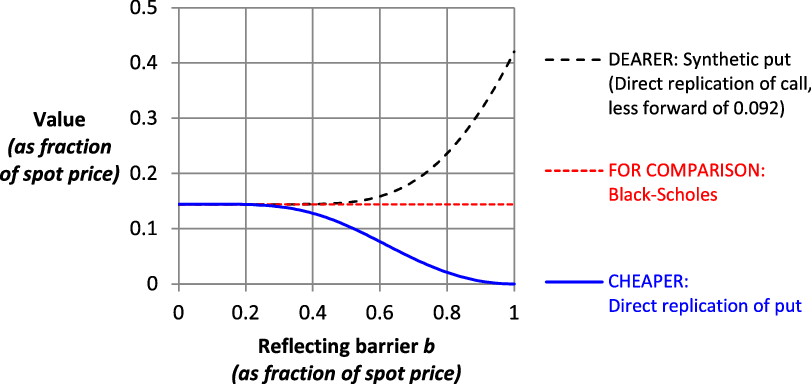
Figure 7. Put option: direct replication is cheaper than synthetic replication.
For a put, direct replication is always cheaper than synthetic replication. To understand this, note that the cheaper replication strategy is the one that is better positioned at the barrier. Then, observe that the deltas of the two replication strategies when the spot price touches the barrier at an interim time t are:
synthetic replication: $\delta \!\left( {{C_B} - {}^S{F_B}} \right) = {\delta _{{C_B}}} - \;{e^{ - q\left( {T - t} \right)}} = - \;{e^{ - q\left( {T - t} \right)}}$
direct replication: ${\delta _{{P_B}}} = \;\;0$
.
${\delta _{{P_B}}} = \;\;0$
.
So the synthetic strategy is always badly positioned at the barrier (short the asset, which is subject to positive interventions). This makes it more expensive.
The dashed straight red line representing the Black-Scholes price (i.e. ignoring the barrier) is shown in Figure 7 mainly to illustrate that our preferred valuation, the blue line ${P_B}$
, sensibly converges to the Black-Scholes price for b = 0. But perhaps surprisingly, replication based on the Black-Scholes delta will also exactly replicate option payoffs in the presence of a barrier b > 0, albeit at unnecessarily high cost. For a discussion of this point, please see Appendix B (Supplementary Material).
${P_B}$
, sensibly converges to the Black-Scholes price for b = 0. But perhaps surprisingly, replication based on the Black-Scholes delta will also exactly replicate option payoffs in the presence of a barrier b > 0, albeit at unnecessarily high cost. For a discussion of this point, please see Appendix B (Supplementary Material).
Another way of seeing that a put should be priced by direct replication is to note that a put is a bounded claim with a maximum payoff of K – b, and then consider the following extreme cases:
-
(i) Barrier equal to strike
For K = b, the put payoff becomes zero. In Figure 7, the strike is 1, and the direct replication price
${P_B}$
(blue line) goes to zero for b = 1, which is intuitively sensible. In contrast, the synthetic replication price
${}^S{P_B}$
(dashed black line) and Black-Scholes price (dashed red line) remain well above zero for b = 1. -
(ii) High volatility
For high volatility (e.g. σ > 0.290 in Figure 7), the synthetic replication price
${}^S{P_B}$
can exceed the maximum possible put payoff K – b. But this gives an immediate arbitrage, with no credit requirements: write the put for a cash credit of
${}^S{P_B}$
, which is larger than the maximum possible payoff you need to make. In contrast, the direct replication price
${P_B}$
is well-behaved for high volatility: it increases modestly towards a limit, but remains less than the Black-Scholes price.


5. Illustration for a Call Option
5.1. With no margin requirements: synthetic replication is preferred
Figure 8 illustrates the comparative costs of direct replication ${C_B}$
and synthetic replication
${C_B}$
and synthetic replication ${}^S{C_B}$
for a call option with the same parameters as in section 4, for a range of barrier levels.
${}^S{C_B}$
for a call option with the same parameters as in section 4, for a range of barrier levels.
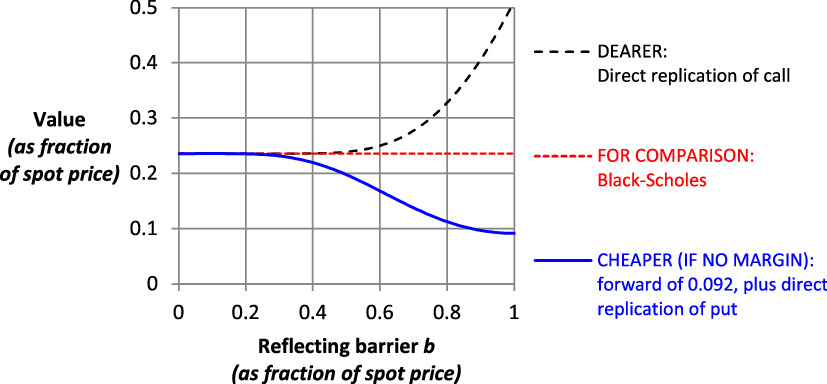
Figure 8. Call option: synthetic replication is cheaper than direct replication.
We can make the following observations on Figure 8.
For a call, if we assume m = 0 (i.e. no margin payments are required on interim losses of replication), synthetic replication always has a lower initial cost than direct replication. To understand this, note that the deltas of the replication strategies when the spot price touches the barrier at an interim time t are:
synthetic replication: $\delta \!\left( {{}^S{F_B} + {P_B}} \right) = {e^{ - q\left( {T - t} \right)}} + {\delta _{{P_B}}} = {e^{ - q\left( {T - t} \right)}}$
direct replication: ${\delta _{{C_B}}} = \;\;0$
So the synthetic replication strategy is always better positioned at the barrier (long the asset, which is subject to positive interventions).
It may seem counter-intuitive to say that in a world with a higher barrier, a call can be replicated at lower cost (as a fraction of the initial spot price)Footnote
16
. To understand this, look at Figure 9. This shows four possible paths for the notional price N
t
and the corresponding observed price S
t
(in the upper left panel, there are no barrier touches, so the two paths never diverge). In each panel, the effect of the intervention on the terminal price is ${S_T} - {N_T}$
, and the effect on the call payoff is:
${S_T} - {N_T}$
, and the effect on the call payoff is:
-
(i) upper left panel: no increase (because no barrier touches, so no interventions)
-
(ii) upper right panel: increase of
${S_T} - {N_T}$
; -
(iii) lower left panel: increase of less than
${S_T} - {N_T}$
; -
(iv) lower right panel: no increase (because terminal observed price below strike).


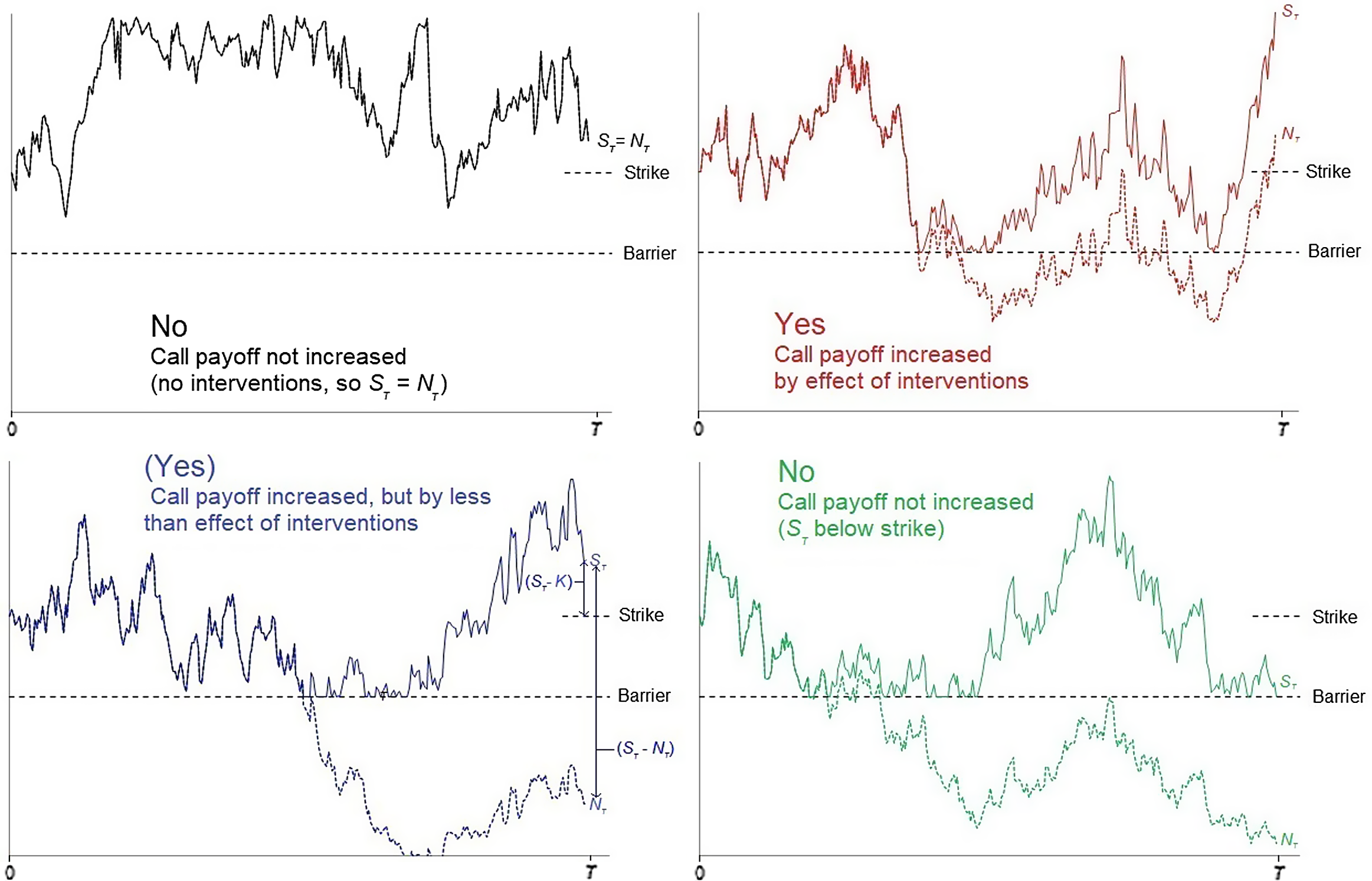
Figure 9. Call payoff, $\max\! \left( {{S_T} - K,0} \right)$
, may be less than accumulated effect of the interventions.
$\max\! \left( {{S_T} - K,0} \right)$
, may be less than accumulated effect of the interventions.
We can then see that the reduction in call replication cost, compared to a world with no barrier, arises from paths of type (iii). For these paths, the synthetic replication strategy ${}^S{C_B}$
fully captures the effect of the interventions, but the call payoff is increased by less than the effect of the interventions. As foreshadowed graphically in section 3.1, a call is an “inefficient” contract in the presence of the barrier.
${}^S{C_B}$
fully captures the effect of the interventions, but the call payoff is increased by less than the effect of the interventions. As foreshadowed graphically in section 3.1, a call is an “inefficient” contract in the presence of the barrier.
We can usefully consider the same extreme cases for the call as we did for the put:
-
(i) Barrier equal to strike
For K = b, the call is economically equivalent to a forward contract. The synthetic replication price
${}^S{C_B}$
then sensibly prices the call as a forward contract, (i.e.
${P_B} = 0$
, so
${}^S{C_B} = {}^S{F_B}$
); but the direct replication price
${C_B}$
gives an unnecessarily higher price. -
(ii) High volatility
For high volatility (e.g. σ > 0.409 in Figure 8), the direct replication price
${C_B}$
exceeds the spot price. This gives an immediate arbitrage, with no credit requirement: write the call and buy the stock for a cash credit
${C_B} - S$
, and then at maturity either deliver the stock and receive the strike (if the call is exercised), or keep the original cash credit (if the call is not exercised). On the other hand, the synthetic replication price
${}^S{C_B}$
sensibly remains less than the spot price for all volatilities.


5.2. With margin requirements: call price is ambiguous
The synthetic replication strategy ${}^S{C_B}$
is subject to the caveat discussed in section 3, i.e. the interim losses can exceed the initial saving
${}^S{C_B}$
is subject to the caveat discussed in section 3, i.e. the interim losses can exceed the initial saving ${C_B} - {}^S{C_B}$
plus interest to the interim date. This is more likely when the barrier is low, towards the left of Figure 8: the initial saving (i.e. the gap between the black and blue curves) is small, and the largest possible interim loss is large. To illustrate, let
${C_B} - {}^S{C_B}$
plus interest to the interim date. This is more likely when the barrier is low, towards the left of Figure 8: the initial saving (i.e. the gap between the black and blue curves) is small, and the largest possible interim loss is large. To illustrate, let ${V_t}\!\left( {{}^SC_B^{\,t}} \right)$
be the value of the synthetic replicating portfolio for a call at interim time t, and define the “Interim Loss Ratio” (ILR) of the strategy as
${V_t}\!\left( {{}^SC_B^{\,t}} \right)$
be the value of the synthetic replicating portfolio for a call at interim time t, and define the “Interim Loss Ratio” (ILR) of the strategy as
 \begin{align} {\rm{ILR}} = \mathop {\min }\limits_{0\, \le \,t\, \le T} \!\left( {\frac{{{V_t}\!\left( {{}^SC_B^{\,\,t}} \right)}}{{\!\left( {{C_B} - {}^S{C_B}} \right)\!{e^{rt}}}}} \right)\end{align}
where ILR < −1 indicates that the negative value of the strategy exceeds the rolled-up initial saving at some point during the term. Then on the assumptions at the start of section 2.3 (in particular, S = K = 1), for b = 0.7, the 25% conditional tail expectation of the ILR is −0.76 (and none of 10,000 simulations gives ILR < −1). So for b ≥ 0.7, strategy ${}^S{C_B}$
might be preferred: the maximum possible interim loss is smaller than the rolled-up difference in initial costs. But for b = 0.6, 0.5, 0.4, the corresponding 25% tail expectations of the ILR are −1.53, −2.98, −5.20. For these cases, the strategy
${}^S{C_B}$
might be preferred: the maximum possible interim loss is smaller than the rolled-up difference in initial costs. But for b = 0.6, 0.5, 0.4, the corresponding 25% tail expectations of the ILR are −1.53, −2.98, −5.20. For these cases, the strategy ${C_B}$
might be preferred: it has a slightly higher initial cost, but avoids a substantial chance of interim losses of several times the extra cost.
${C_B}$
might be preferred: it has a slightly higher initial cost, but avoids a substantial chance of interim losses of several times the extra cost.
To summarise this section: ignoring margin requirements, the initial cost of synthetic replication ${}^S{C_B}$
is always cheaper than that of direct replication
${}^S{C_B}$
is always cheaper than that of direct replication ${C_B}$
. But the strategy
${C_B}$
. But the strategy ${}^S{C_B}$
may have negative value at interim dates, and these losses can be much larger than the difference in initial costs plus interest to the interim date. If margin payments need to be made to cover interim losses, the price of a call seems ambiguous.
${}^S{C_B}$
may have negative value at interim dates, and these losses can be much larger than the difference in initial costs plus interest to the interim date. If margin payments need to be made to cover interim losses, the price of a call seems ambiguous.
6. Arbitrage and Limits to Arbitrage
The dual replicating strategies for puts, calls and forwards as discussed above point to the possibility for arbitrage strategies in the barrier model. This section examines these possibilities directly, and their practicality in the context of credit constraints.
6.1. Buying when the spot price touches the barrier (not feasible)
Theoretically, if we could buy at the instant when S t touches the barrier, and sell immediately after reflection, this would be an immediate arbitrage, with no risk of interim losses. However, we have already noted in section 2.1 that this is not practically feasible: the spot price spends no finite time at the barrier, so no-one can implement the strategy. From a mathematical viewpoint, the existence of this strategy has consequences: it rules out the existence of an equivalent martingale measure for the asset price. But from an economic viewpoint, a purely theoretical arbitrage opportunity seems of no consequence: if no-one can implement the arbitrage, it cannot affect the assumed price processFootnote 17 .
Although buying exactly when S t touches the barrier is not feasible, it may be possible to obtain some sort of approximation. Intuitively, we can do this by increasing a long position as S t approaches the barrier, and then reducing the position as S t moves away from the barrier. This type of strategy will be exposed to interim losses, because S t can fall further after we initiate the position, but the presence of the barrier will place a limit on the losses. All the strategies discussed below amount to some form of this approximation.
6.2. Net-delta strategy (arbitrage with interim losses)
In Figure 6, the pairs of replicating paths for forward, put and call all have the same initial difference, ${F_B} - {}^S{F_B}$
(which is independent of the strike K), and the differences shrink at the same rate in each panel as the replicating paths converge on the contract payoff. This is because the duality of replicating paths in each panel has the same underlying cause: the forward contract payoff can be replicated either in a cheaper way which exploits the interventions (
${F_B} - {}^S{F_B}$
(which is independent of the strike K), and the differences shrink at the same rate in each panel as the replicating paths converge on the contract payoff. This is because the duality of replicating paths in each panel has the same underlying cause: the forward contract payoff can be replicated either in a cheaper way which exploits the interventions ( ${}^S{F_B}$
), or in a dearer way which does not (
${}^S{F_B}$
), or in a dearer way which does not ( ${F_B}$
). It follows that if we run the cheaper strategy long and the dearer strategy short, we should be able extract the initial difference in prices
${F_B}$
). It follows that if we run the cheaper strategy long and the dearer strategy short, we should be able extract the initial difference in prices ${F_B} - {}^S{F_B}$
(also equal to
${F_B} - {}^S{F_B}$
(also equal to ${C_B} - {}^S{C_B}$
and
${C_B} - {}^S{C_B}$
and ${}^S{P_B} - {P_B}$
) plus interest over the term. Because the two strikes are equal and opposite, they do not need to be replicated; we can just do the delta trading on each side, funded wholly by borrowing. That is, starting from zero wealth, we borrow to fund a continuously varying “net-delta” position Δ, specified by differentiating minus Equation (27) with respect to the asset price:
${}^S{P_B} - {P_B}$
) plus interest over the term. Because the two strikes are equal and opposite, they do not need to be replicated; we can just do the delta trading on each side, funded wholly by borrowing. That is, starting from zero wealth, we borrow to fund a continuously varying “net-delta” position Δ, specified by differentiating minus Equation (27) with respect to the asset price:
 \begin{align} \quad \quad \quad \Delta = \frac{\partial }{{\partial S}}\!\left( {{}^s{F_B} - {F_B}} \right) = {e^{ - qT}}\left\{ {1 - \Phi\!\left( {{z_3}} \right) + {{\left( {\frac{b}{S}} \right)}^{1 + \theta }}\Phi\!\left( {{z_4}} \right)} \right\}\end{align}
which is always a long position, and gives the same terminal payoff whether or not the barrier is touched. The terminal payoff is a constant representing the $\mathbb{Q}$
N
-expectation of the effect of the interventions on the terminal asset price (i.e. the effect anticipated in our proposed option prices). The strategy reaches its maximum long position when the asset is at the barrier: it buys at an increasing rate as the asset approaches the barrier and sells at a decreasing rate as it rebounds, and so approximates a purchase exactly at the barrier.
$\mathbb{Q}$
N
-expectation of the effect of the interventions on the terminal asset price (i.e. the effect anticipated in our proposed option prices). The strategy reaches its maximum long position when the asset is at the barrier: it buys at an increasing rate as the asset approaches the barrier and sells at a decreasing rate as it rebounds, and so approximates a purchase exactly at the barrier.
The viability of this strategy is investigated in Appendix C (Supplementary Material). In summary:
-
(i) The strategy is difficult to scale if initiated when the spot price is well above the barrier, because the potential interim losses are very large relative to the terminal gain, especially when the strategy is run over shorter terms.
-
(ii) It becomes more scalable if initiated when the spot price is already close to the barrier. This is intuitive: the closer to the barrier a long position is initiated, the less it can lose.
-
(iii) To the extent that the strategy is implemented near the barrier, this may disrupt the assumed price process near the barrier. But this has little effect on the replication of a put, because
${\delta _{{P_B}}} \to 0\;{\rm{as}}\;S \to b$
, so that the put replicating portfolio
${P_B}$
has almost no exposure to the asset price near the barrier. -
(iv) Point (iii) also addresses the more general criticism that even market participants who do not pursue explicit arbitrage strategies may tend to buy as the spot price approaches the barrier, thus modifying the price process in this region. Yes, this may be so; but because the put replication portfolio has almost no exposure to the asset in this region, it makes little difference to the replication of a put.


6.3. Call paradoxes
The synthetic replication strategy for a call captures the full benefit of the interventions at the barrier along all possible paths for the asset, irrespective of the option strike. For a high strike, the $\mathbb{Q}$
N
-expectation of the call payoff tends to zero. It follows that the payoff can be funded starting from wealth of minus the discounted
$\mathbb{Q}$
N
-expectation of the call payoff tends to zero. It follows that the payoff can be funded starting from wealth of minus the discounted $\mathbb{Q}$
N
-expectation of the interventions. Stated differently, for a high strike, the synthetic replication strategy
$\mathbb{Q}$
N
-expectation of the interventions. Stated differently, for a high strike, the synthetic replication strategy ${}^S{C_B}$
tends to the net-delta arbitrage strategy in Equation (30), so we can start with wealth of minus the certain gain this will make.
${}^S{C_B}$
tends to the net-delta arbitrage strategy in Equation (30), so we can start with wealth of minus the certain gain this will make.
However, the putative “negative price” just suggested assumes that the call writer replicates by the synthetic replication strategy ${}^S{C_B}$
. This involves interim losses, which for a high strike can be a large multiple of the negative initial cost (particularly if the initial spot price is well above the barrier, as noted at 6.2(i) above). In contrast, the direct replication strategy
${}^S{C_B}$
. This involves interim losses, which for a high strike can be a large multiple of the negative initial cost (particularly if the initial spot price is well above the barrier, as noted at 6.2(i) above). In contrast, the direct replication strategy ${C_B}$
avoids any possibility of interim losses, and as we increase the strike, its initial cost tends to zero from above. As previously noted, the choice between the two strategies (and hence the price of a call) seems ambiguous. It may be reasonable to assume that in practice (a) any offered prices for calls will be strictly positive, but (b) there may be few buyers of calls with high strikes, because the payoff can potentially be replicated more cheaply (albeit with interim losses). In other words, calls with high strikes are likely to be illiquid.
${C_B}$
avoids any possibility of interim losses, and as we increase the strike, its initial cost tends to zero from above. As previously noted, the choice between the two strategies (and hence the price of a call) seems ambiguous. It may be reasonable to assume that in practice (a) any offered prices for calls will be strictly positive, but (b) there may be few buyers of calls with high strikes, because the payoff can potentially be replicated more cheaply (albeit with interim losses). In other words, calls with high strikes are likely to be illiquid.
The negative initial cost of replication (ignoring interim losses) for high strikes can also be understood graphically by looking at Figure 9. We have already noted that for paths of the lower left type, the call payoff is less than the quantum of the accumulated interventions, ${S_T} - {N_T}$
. Now think about what happens as the strike rises. The density of the types of paths shown in the top two panels falls: because the strike is high, very few of the underlying GBM paths for the notional price N
t
terminate above the strike. All the call payoff then arises from paths of the advantageous lower left type, where the payoff is more than fully funded by the free interventionsFootnote
18
.
${S_T} - {N_T}$
. Now think about what happens as the strike rises. The density of the types of paths shown in the top two panels falls: because the strike is high, very few of the underlying GBM paths for the notional price N
t
terminate above the strike. All the call payoff then arises from paths of the advantageous lower left type, where the payoff is more than fully funded by the free interventionsFootnote
18
.
The “high” strike postulated above is, more precisely, high relative to the forward price of $S{e^{\left( {r - q} \right)T}}$
. It follows that a negative call replication cost can also arise for q > r, or S sufficiently close to b. These effects can be understood as follows.
$S{e^{\left( {r - q} \right)T}}$
. It follows that a negative call replication cost can also arise for q > r, or S sufficiently close to b. These effects can be understood as follows.
For q > r, a debt-funded long position initiated sufficiently close to the barrier is an arbitrage: the barrier ensures that maximum possible capital loss at maturity is less than the accumulation of the carry q – r. Interim losses can occur, because the spot price can move closer to the barrier before much carry has accumulated, but the barrier limits the size of these losses.
For $S\; \to \;b$
, in terms of Figure 9, if S
t
is already close to the barrier, there will be a high density of future asset paths that receive a significant contribution from interventions at the barrier. Most asset price paths that produce positive call payoffs will then be of the advantageous lower left type.
$S\; \to \;b$
, in terms of Figure 9, if S
t
is already close to the barrier, there will be a high density of future asset paths that receive a significant contribution from interventions at the barrier. Most asset price paths that produce positive call payoffs will then be of the advantageous lower left type.
There is a possible economic interpretation of the negative call price. For a sufficiently strong combination of q > r and $S\; \to \;b$
, a long position in the asset funded wholly by debt can be entered at zero cost and gives a certain gain (provided that the margin requirement can be financed). A call option may then be a less attractive proposition than the zero-cost long position (especially for higher strikes, which make a positive call payoff less likely).
$S\; \to \;b$
, a long position in the asset funded wholly by debt can be entered at zero cost and gives a certain gain (provided that the margin requirement can be financed). A call option may then be a less attractive proposition than the zero-cost long position (especially for higher strikes, which make a positive call payoff less likely).
Any potential exploitation of the paradoxes highlighted in this section implies disruption of the assumed asset price process near the barrier. But as we have already noted in section 6.2(iv), the put replicating portfolio has almost no exposure to the asset in this region, so the exploitation should make little difference to the replication of a put.
6.4. Bounds on option prices
The modified form of put-call parity suggested in Equation (28):
 \begin{align} {}^S{C_B} - {P_B} = {}^S{F_B}\end{align}
Synthetic call price – Direct put price = Sub-martingale forward price
invalidates the standard lower bound: ${\rm{Put}}\; \geq \max\! \left( {K{e^{ - rT}} - S{e^{ - qT}},0} \right)$
. This bound is often described as “model-free,” but it depends on the standard put-call parity, and is not implied by the modified parity above. To see the invalidity of the standard lower bound, consider a put with a strike equal to the barrier, K = b. This put can never have any payoff, and so is sensibly valued at zero, as given by our formula P
B
; but if S is close to the barrier with K = b and r < q, the standard lower bound will be well above zero.
${\rm{Put}}\; \geq \max\! \left( {K{e^{ - rT}} - S{e^{ - qT}},0} \right)$
. This bound is often described as “model-free,” but it depends on the standard put-call parity, and is not implied by the modified parity above. To see the invalidity of the standard lower bound, consider a put with a strike equal to the barrier, K = b. This put can never have any payoff, and so is sensibly valued at zero, as given by our formula P
B
; but if S is close to the barrier with K = b and r < q, the standard lower bound will be well above zero.
For a call, the standard lower bound is ${\rm{Call}} \geq \max\! \left( {S {e^{ - qT}} - K {e^{ - rT}},0} \right)$
. The first limit remains valid in the presence of the barrier:
${\rm{Call}} \geq \max\! \left( {S {e^{ - qT}} - K {e^{ - rT}},0} \right)$
. The first limit remains valid in the presence of the barrier: ${}^S{C_B} \geq S {e^{ - qT}} - K {e^{ - rT}}$
, i.e. a call has optionality, so it is worth at least as much as a forward with the same strike. The second limit of zero is reasonable for offered prices of calls, albeit these will probably be illiquid, as discussed in section 6.3 above.
${}^S{C_B} \geq S {e^{ - qT}} - K {e^{ - rT}}$
, i.e. a call has optionality, so it is worth at least as much as a forward with the same strike. The second limit of zero is reasonable for offered prices of calls, albeit these will probably be illiquid, as discussed in section 6.3 above.
The inapplicability of the standard lower bound for a put also implies a modification to the standard upper bound for the valuation of an equity release mortgage, as in the “Principle II” promulgated by the Prudential Regulation Authority (2020) in the United Kingdom. This is covered in Appendix D (Supplementary Material).
7. Discussion
7.1. Mathematical versus economic perspectives on arbitrage
When considering the consequences of the various arbitrage possibilities in highlighted in section 6, it is useful to distinguish between mathematical and economic perspectives.
From a mathematical perspective, the feasibility of any form of arbitrage, even if incapable of practical implementation, negates the “No Free Lunch With Vanishing Risk” condition in the fundamental theorem of asset pricing (Delbaen & Schachermayer, Reference Delbaen and Schachermayer1994). It follows by the theorem that no equivalent martingale measure for the observed asset price S t exists; this negates the usual justification for using the computational technique of risk-neutral pricing. But in the barrier model, there is a different justification: we can apply risk-neutral arguments at the level of the notional price N t (not the observed price S t ), but then nevertheless hedge using S t , as explained in section 2.4.
From an economic perspective, the feasibility of arbitrage suggests that the assumed price process for S t might not be realistic, insofar as the actions of arbitrageurs may tend to eliminate the features which arbitrage exploits. But the importance of this economic concern depends on the extent to which the arbitrage can be scaled, and whether this eliminates the regularity which it exploits. On this, the following points can be made.
-
(1) The arbitrage represents a disequilibrium in the barrier model. But it is a disequilibrium funded by the government, and therefore, by assumption, a sustainable one. This sustainability derives from the government’s unlimited powers of intervention, as detailed in the next point.
-
(2) Whilst the existence of an explicit barrier would imply arbitrage opportunities as identified in section 6, the barrier is in reality not an explicit feature. Instead, it is a metaphor for the full range of possible policy responses to a large fall in house prices: changes in general monetary and fiscal policies, relaxation of prudential limits on mortgage lending, interest-free and/or non-recourse State loans to house purchasers, regulatory changes which incentivise or compel institutional investors to buy houses, printing money to buy houses, etc. The metaphorical nature of the barrier precludes arbitrage in practice.
-
(3) The arbitrage opportunities all involve interim losses (except for the impractical one of buying when the spot price is exactly at the barrier). Appendix C (Supplementary Material) shows that the credit requirements are generally substantial relative to the gains, and so the ability to scale the arbitrages will be limited by credit constraints. The credit requirements can be reduced by initiating the strategy only when the spot price is already very close to the barrier (essentially mimicking a purchase exactly at the barrier). But disruption to the price process in this region makes almost no difference to the replication of a put, because the put delta near the barrier is very close to zero.
-
(4) A number of authors have put forward models where credit constraints, margin requirements and other institutional features lead to the persistence of some arbitrage opportunities in equilibrium, e.g. Shleifer & Vishny (Reference Shleifer and Vishny1997), Loewenstein & Willard (Reference Loewenstein and Willard2000), Basak & Croitoru (Reference Basak and Croitoru2000), Liu & Longstaff (Reference Liu and Longstaff2004). Others have documented empirical evidence of persistent arbitrages in various markets, e.g. Gemmill & Thomas (Reference Gemmill and Thomas1997), Lamont & Thaler (Reference Lamont and Thaler2003), Mitchell et al. (Reference Mitchell, Pedersen and Pulvino2007), Mitchell & Pulvino (Reference Mitchell and Pulvino2012).
-
(5) Experience with currency barriers suggests that when the spot price approaches a lower barrier, there is often increased selling (not buying, as the logic of arbitrage would suggest), presumably predicated on speculation that the authorities may not continue to support the barrier. For example, Hertrich & Zimmerman (Reference Hertrich and Zimmermann2017) find that currency option prices shortly before the Swiss National Bank abandoned its lower barrier for the Euro/Swiss Franc rate in January 2015 were consistent with the put formula assuming a “true” barrier significantly below the official policy barrier. To the extent that such speculative selling occurs, it may offset any buying predicated on the logic of arbitrage.
7.2. Alternatives to the barrier model
The complications identified in this paper make the barrier model seem more conditional on practical limits to arbitrage than was apparent in previous papers (Veestraeten, Reference Veestraeten2008, Reference Veestraeten2013; Hertrich, Reference Hertrich2015; Hertrich & Zimmermann, Reference Hertrich and Zimmermann2017; Thomas, Reference Thomas2021). However, I suggest that its usefulness in applications such as NNEG valuation should be judged by comparison with available alternatives, not an abstract standard of perfection that no extant model attains. If one believes that the barrier assumption, or something like it, is a closer approximation of reality for house prices over the long term than an unrestricted geometric Brownian motion (for reasons, see Thomas, Reference Thomas2021, sections 2 and 3), there do not seem to be any wholly satisfactory approaches. Three possible alternatives are as follows.
-
(i) Standard Black-Scholes, as prescribed by the Prudential Regulatory Authority (2020) for NNEG valuation for certain regulatory purposes. This simply ignores the reality that interventions are likely after large falls in prices, and produces what one well-known writer of long-dated puts has called “wildly inappropriate values when applied to long-dated options” (Buffett, Reference Buffett2011). In the context of NNEG, Black-Scholes seems to me a short-term model stretched well beyond its sensible range of application, like trying to use an egg-timer as a calendar.
-
(ii) The “real-world” method typically used by UK insurers for NNEG valuation (Hosty et al., Reference Hosty, Groves, Murray and Shah2008). This makes an ad hoc adjustment to the Black-Scholes formula, replacing the forward house price
$S{e^{\left( {r - q} \right)T}}$
with a projected house price
$S{e^{g\,T}}$
, where g > r – q. This gives much lower put values than Black-Scholes. If calls are also valued by this method, then to be consistent with parity, the forward price must be
$S{e^{g\,T}}$
(this can be seen by reworking Equation (21) with r – q replaced by g, and is also discussed in Taleb, Reference Taleb2015). The real-world method therefore implicitly assumes the persistence of a large static arbitrage (i.e. parity-implied forward price
$S{e^{g\,T}}$
less no-arbitrage forward price
$S{e^{\left( {r - q} \right)T}}$
). This might be considered a more disconcerting assumption than the persistence of some limited dynamic arbitrage in the barrier model.To illustrate, in the representative example detailed in section 2.3 (in particular S = K = 1, b = 0.5), the value at inception of the arbitrage in the barrier model is 0.0416; this can be extracted only by a dynamic strategy that may incur substantial interim losses. But in the real-world model with a typical house price growth g = 2.5% and all other parameters the same, the value at inception of the arbitrage is 0.5052 (i.e. 12x larger); this can be extracted by a static strategy with no interim losses.
-
(iii) The benchmark approach originated by Eckhard Platen (e.g. Platen, Reference Platen2002; Buhlmann & Platen, Reference Buhlmann and Platen2003; Platen & Heath, Reference Platen and Heath2010; Fergusson & Platen, Reference Fergusson and Platen2022). This involves a change of numeraire to the “benchmark portfolio” which maximises expected log-utility of terminal wealth (in other literature, the “growth optimal portfolio”). The price of an option is then defined as its real-world conditional expectation in the benchmark numeraire; for long terms, the price is significantly less than Black-Scholes. Effectively, the benchmark approach anticipates the asset’s risk premium in general, rather than the prospect of intervention after a large fall in prices. There is no equivalent martingale measure, so some arbitrage is possible, but only with interim losses. There are some apparent paradoxes, but different ones from the barrier model: the price of a put approaches zero when the benchmark portfolio is low, and a modified form of put-call parity applies.


Notably, all of the barrier, real-world and benchmark models allow some form of arbitrage. This perhaps reflects an implicit view that the persistence of some arbitrage opportunities may be a reasonable feature of a long-term asset model, if the ability to scale them in practice is curtailed by credit limits, transaction costs, and other institutional constraints.
8. Conclusions
Putting sections 2–7 together, we can state the following conclusions.
-
(1) The observed price process S t (a reflected geometric Brownian motion) in the barrier model is not arbitrage-free. Arbitrage with interim losses is possible (or with no losses if one could buy exactly at the barrier, but this can never be implemented in practice).
-
(2) The arbitrage possibilities represent a disequilibrium in the barrier model. But it is a disequilibrium funded by the government, and therefore (by assumption) a sustainable one, based on the government’s unlimited powers of intervention.
-
(3) The possibility of arbitrage, whether or not it is implemented, implies (by the Fundamental Theorem of Asset Pricing) that there is no change of measure that will make the observed price S t a martingale. So the usual justification for risk-neutral option valuation does not apply to options on S t .
-
(4) Nevertheless, options on S t can be expressed as compound options on the underlying arbitrage-free notional price N t (a geometric Brownian motion), to which change of measure and other standard risk-neutral arguments can be applied. Although N t is not available for hedging, the required hedging schemes for the compound option have deltas which go to zero whenever N t attains a new minimum below the barrier (equivalently: whenever S t touches the barrier). Then because, everywhere above the barrier, S t is just a piecewise-scaled version of N t , hedging with S t and a piecewise-scaled delta gives the same results as hedging with N t .
-
(5) The price of a put is clear: direct replication has a lower initial cost than synthetic replication, and the replication portfolio always has positive value, so no extra funding is required for interim losses. This affirms the relevance of the cheaper direct replication price
${P_B}$
(rather than the dearer synthetic replication price
${}^S{P_B}$
) for NNEG valuation. -
(6) The price of a call is ambiguous: synthetic replication has a lower initial cost than direct replication, but the replication portfolio may give interim losses. So the preferred replication strategy, and hence price, of a call depends on what margin payments need to be made on these losses.
-
(7) It follows from points (4) to (6) that put-call parity is also in general ambiguous. However, if no margin payments are required on interim losses, we can think of parity as
${}^S{C_B} - {P_B} = {}^S{F_B}$
, that is Synthetic call price – Direct put price = Sub-martingale forward price.
-
(8) Potential arbitrage strategies in the barrier model are all predicated on borrowing to increase a long position as S t approaches the barrier and then reducing the position as S t moves away from the barrier. The practicality of scaling this strategy depends on credit limits and margin requirements. To the extent that arbitrage is implemented (and funded by the government), the assumed price process of reflected geometric Brownian motion may be disrupted, particularly near the barrier.
-
(9) The delta of the direct replication
${P_B}$
for a put tends to zero as the asset price approaches the barrier. This makes the strategy more robust to the possible disruption of the assumed price process near the barrier (as mentioned in the previous point).


Computer code
Code in the R programming language demonstrating Monte Carlo evaluation of the options and the associated replication schemes is available at https://github.com/guythomas7.
Acknowledgements
I wish to thank (without implicating) Markus Hertrich, Alan Reed, and Pradip Tapadar for comments on earlier drafts, and Dean Buckner and Kevin Dowd for useful criticisms of earlier papers.
Supplementary materials
For supplementary material for this article, please visit https://doi.org/10.1017/S1748499522000227


 Open access