


Introduction
In data-driven engineering design, the production of data across a product or system's life cycle is becoming abundant (McAfee and Brynjolfsson, Reference McAfee and Brynjolfsson2012). Data are generated from multiple sources, and it is becoming a common design practice to integrate sensors in products as well as product manufacturing. Simultaneously, with the advances in data analytics, the practices followed at different stages of product design are undergoing a transition. The discipline relies extensively on simulations to replace expensive prototyping. Simulation-based design evaluation is increasingly used when the cost of prototyping complex systems is high (Li et al., Reference Li, Zhao and Shao2012). However, simulations may become tedious and expensive when a large design space needs to be evaluated (Choi et al., Reference Choi, Lee and Kim2014). In that context, generating metamodels is often a suitable alternative. Metamodels are simplified models representing the essence of complex phenomena or complex simulation models (Bhosekar and Ierapetritou, Reference Bhosekar and Ierapetritou2018). In a production environment, it is advantageous to produce metamodels using machine learning methods because of its automation capabilities (Reference Cai, Ren, Wang, Xie, Zhu and GaoCai et al., n.d.; Sun and Wang, Reference Sun and Wang2019).
In data-driven design, the product development process should benefit from tools and approaches that can extract and integrate useful knowledge embedded in the data to produce models (Berman, Reference Berman2013; Brunton and Kutz, Reference Brunton and Kutz2019; Lee et al., Reference Lee, Cooper, Hands and Coulton2022). It will be beneficial for developed models to support reasoning through simulation. Simulation-based reasoning is a significant contribution to the early decision-making process (Felsberger et al., Reference Felsberger, Oberegger and Reiner2016). The decision-making process relies on human judgment and its global acceptance in any organization requires the production of rationales supporting the decisions (Chaudhuri et al., Reference Chaudhuri, Dayal and Narasayya2011). Models should facilitate the human cognitive processes (Miller, Reference Miller1956; Dadi et al., Reference Dadi, Goodrum, Taylor and Carswell2014). In human cognition, a natural tendency for humans is to develop a causal interpretation of events. Such causal interpretations can be valid or erroneous, but they represent a strong human cognitive pattern. Any tools developed to support decision making should also consider the human characteristic. Approaches such as graph-based representations and causal ordering for parsimonious models produced can facilitate the model's transparency and enable efficient human decision-making by being aligned with the human cognition (Goel et al., Reference Goel, Vattam, Wiltgen and Helms2012; Shekhawat et al., Reference Shekhawat, Jain, Bisht, Kondaveeti and Goswami2021).
The current research aims to leverage the potential of machine learning for the extraction and integration of knowledge gathered from different data sources in the development of engineering models matching human cognition and supporting automatic reasoning. In general terms, knowledge can be defined as awareness of facts or as practical skills. It may also refer to familiarity with objects or situations. Knowledge of facts is distinct from opinion because it benefits from justification provided through rationales. Such rationales are produced using a representation of the knowledge or the structure of knowledge which can be easily shared and understood. This research exploits two sources of knowledge, namely, data collected from a system and the fundamental units of the variables of the system. The article presents a two-part method for generating a structure of knowledge. First, oriented graphs representing the variables of the dataset as nodes and their interrelations as edges are developed. Second, a power-law representation is developed for the variables of the system. The power laws and the oriented graphs are composed together to construct the structure of knowledge wherein, the exponents of the power laws being associated with the nodes (i.e., the variables) and the multiplicative connections between variables are associated with the edges (i.e., variable interrelationships).
This research aims to extend the scope of the pre-existing dimensional analysis conceptual modeling framework (DACM) to develop oriented graphs. The goal is to exploit datasets as a new form of inputs for the framework. The DACM framework has been initially developed for generating oriented graphs combined with power-law equations using functional representation as a starting point for modeling of systems (Mokhtarian et al., Reference Mokhtarian, Coatanéa and Paris2017). Initially, it was developed for bringing simulation to the very early stage of the engineering design process. In the framework, a mathematical machinery based on qualitative reasoning using power laws has been implemented to incorporate qualitative objectives in the developed models (Bhaskar and Nigam, Reference Bhaskar and Nigam1990). The DACM propagation algorithm can propagate qualitative objectives into oriented graphs and detect physical contradictions as defined in theory of inventive problem solving (TRIZ) (Savransky, Reference Savransky2000). This is allowing the detection of design weaknesses at the early design conceptual stage (Eckert et al. Reference Eckert, Kelly and Stacey1999; Shahin, Reference Shahin2008; Jin and Benami, Reference Jin and Benami2010). TRIZ separation principle (Savransky, Reference Savransky2000) is used to modify the topology of the oriented graphs and consequently generate innovative solutions minimizing or removing the contradictions for ultimately creating better designs (Kryssanov et al., Reference Kryssanov, Tamaki and Kitamura2001; Mayda and Börklü, Reference Mayda and Börklü2014). However, to be able to generate a valid reasoning with this approach, a pre-requisite is to build the oriented graph to accurately represent the causal relationships in the system of interest. In the case of the exploitation of a dataset as the initial starting knowledge, classical machine learning methods cannot guarantee the validity of the causal ordering. Thus, the proposed method enables the development of oriented graphs with an accurate causal ordering of variables which can then be used in tandem with the DACM framework for qualitative reasoning.
The integration and exploitation of data in the DACM framework can provide a standardized way to approach early design reasoning; however, the usability of the models may be affected by the model fidelity. The objectives of the model and the designer, and relevant applications must be considered when developing engineering models (Ponnusamy et al., Reference Ponnusamy, Albert and Thebault2014). As mentioned above, a valid causal ordering is a necessary condition for qualitative reasoning using the DACM framework. Similarly, a lack of standardized approaches to integrate fidelity in modeling approaches can have detrimental effects, weakening the usability of the engineering models. Like fields such as metrology, which is constructed around standardized measurement approaches and fundamental concepts, the design of simulation models for engineering purposes, must also be facilitated by formalization and conceptualization to enable fidelity assessments. The problem has been recognized and an effort to formalize the discipline is ongoing in literature (Gross, Reference Gross1999; Gross et al., Reference Gross, Tucker, Harmon and Youngblood1999; Ponnusamy et al., Reference Ponnusamy, Albert and Thebault2014). In line with existing research, the current article develops a standardized process for machine learning-based modeling to develop simulation models and measure fidelity. The developed models are based on a causal representation of the system variables and can be used for engineering design reasoning and decision making.
The remainder of the article is organized as follows: Section “Background” presents the background on the development of simulation models and evaluation of fidelity. Section “Method” presents the modeling method with the help of a case study. DACM combined with a machine learning module is presented as a model creation and fidelity measurement approach. Section “Case study” presents the findings of this research and the potential applications of the developed approach. Section “Discussion and future work” discusses the conclusions and future development efforts.
Background
In this section, the importance of early decisions in engineering design are emphasized. DACM as a causal ordering framework is briefly introduced. Next, the concept of fidelity in simulation is analyzed and different methods to support the evaluation of some fidelity aspects are presented.
Early design decision support and the role of discovering causal ordering in engineering design and other disciplines
Herbert Simon introduced two concepts relevant for the entire design and manufacturing disciplines. First, the concept of bounded rationality was initially introduced in an economic context as a criticism of the classical economic theory and asserting the existence of a purely rational decision-maker, the homo economicus (Moon, Reference Moon2007). Research in fields such as economics or psychology has demonstrated that rationality is often an exception rather than a norm in human decision processes. Hypothesizing a purely rational behavior is a limitative factor to understanding the complexity of the human decision processes and consequently its branch of design decision making. The second important concept is the concept of satisficing (Simon, Reference Simon1956). The term satisficing is a combination of satisfying and suffice. This concept is important for practical reasons. Indeed, the design activity is a problem-solving activity, where solutions to problems are found in form of tangible or non-tangible artifacts. An artifact is an artificially created object. A satisficing solution to a design problem is a feasible solution produced within specified time limits and using specified and constrained bounded resources.
When working on solutions, certain stages of design can have a higher influence and induce constraints on the final performances of the designed artifacts. For example, design decisions taken at the early stages of the process are less costly but concurrently can also heavily constrain later decisions. Therefore, the early design stage is a strategic phase of the design activity, but also a challenging one, due to the limited availability of early knowledge combined with a high level of associated uncertainty. Early design decisions combine the potential for high added value and high risk due to the ill-defined nature of the early knowledge. Early knowledge combines characteristics such as fuzziness, scarcity, and qualitative nature. Despite the inherent uncertainty, early knowledge can provide crucial information during product development and the potential of this resource is rarely fully exploited in current design practices.
A central aim of the scientific activity is to develop methods to systematically unveil cause–effect relationships between variables of a problem. This is particularly relevant to the engineering design and manufacturing discipline. The discovery of potential confounding variables has been a major source of investigation (VanderWeele and Shpitser, Reference VanderWeele and Shpitser2013). In statistics, a confounding variable is a variable that influences both the dependent and independent variables. This is the source of a false association between variables. Confounding is a concept related to cause–effect relationships and this should not be mixed with the concepts of correlations or relations. The existence of confounders provides rationale for instances when a correlation does not always imply a causal relationship. A variety of approaches have been developed to generate causal ordering in literature (Finkbeiner et al., Reference Finkbeiner, Gieseking and Olderog2015; McCaffrey and Spector, Reference McCaffrey and Spector2018; Bhatt et al., Reference Bhatt, Majumder and Chakrabarti2021). The method proposed in this article contributes to the body of knowledge in causal ordering using oriented graphs and equations. Despite the success of existing causal ordering approaches to be effective and robust in an engineering context, a limiting factor could be the scope of the analysis that could be performed using the causal ordering. Methods such as bond graph causal ordering (Gawthrop and Smith, Reference Gawthrop and Smith1996) or causal ordering of equations via the direct use of Iwasaki and Simon algorithm (Iwasaki and Simon, Reference Iwasaki and Simon1994) or its extensions (Trave-Massuyes and Pons, Reference Trave-Massuyes and Pons1997), as well as work done in qualitative physics (Bhaskar and Nigam, Reference Bhaskar and Nigam1990), are few examples of causal ordering methods belonging to such a classification. Another approach applied more specifically to the social science context is also interesting for this limited literature review. This is a method searching for cause and effect relationships via models using structural equations modeling (SEM) (Pearl, Reference Pearl2000; Spirtes et al., Reference Spirtes, Glymour, Scheines and Heckerman2000). SEM derives from path analysis which was developed by the biologist S. Wright in the 1920s and has been often applied to analyze causal relations of non-experimental data using an empirical approach. Path analysis extends regression analysis by analyzing simultaneously many endogenous and exogenous variables of a system or problem. Path analysis was combined with factor analysis and latent variables to form the SEM approach to causal analysis. In path analysis, variables can be endogenous or exogenous. Relations between variables can be represented by a one-sided arrow when a relationship exists between variables and a two-sided arrow when a correlation exists between variables as presented in Figure 1. Factor analysis is integrated with latent variables in the SEM approach. Factor analysis is a statistical method used to describe variability among observed, correlated variables with the central idea that the variation of observed variables can also be reflecting the variations of unobserved variables name latent variables. Factor analysis may help to deal with datasets where there are large numbers of observed variables that are thought to reflect a smaller number of underlying/latent variables (Harman, Reference Harman1976). However, SEM is of confirmatory nature and researchers have first to model the true causal relationships based on other background knowledge before collecting or analyzing data (Goldberger, Reference Goldberger1972). This task is difficult, especially at the beginning of a design process because of the lack of background initial knowledge.

Fig. 1. Example of an SEM model.
Consequently, using SEM alone, it is often difficult to unveil the initial causal structure. Additionally, SEM suffers from another limitation because SEM assumes normality of the statistical distribution and only uses the covariance structure and cannot find causal direction between two highly correlated variables because the models produced will be equivalent using the SEM approach. Nevertheless, the SEM method constitutes the conceptual basis of several algorithms that are successful in the discovery of causal structure, especially in complex systems studied by sciences such as economics and sociology. This has also been used in medicine and more specifically in epidemiology.
The fundamental concepts of formalism are summarized in the following manner by Halpern (Reference Halpern2000). The construction of structural equations (SE) models requires three key steps. First, the problem being studied is represented by a finite set of variables, corresponding to the features of the problem. This can also be the function of a system to be designed as a solution for a specific design problem (Mobus, Reference Mobus and Mobus2022). There are two sorts of variables. Endogenous variables are such that their values are determined by other variables within the model, whereas the values of exogenous variables are determined in a way that is independent of other variables of the system. The structural equations describe the functional dependence of the endogenous variables on other variables (endogenous and exogenous) in the model (Kaplan, Reference Kaplan2008).
SEM use graphs to represent relations between observed variables and latent variables. Latent variables are not observed. Latent variables can be also residues or errors in the modeling and measurement process. Software specifically developed for SEM are existing to form the model. An SEM can take the following form presented in Figure 1. Each of the generic situations presented above must form each time a specific model. The β is the element of a correlation matrix. The λ is the coefficient allowing to model quantitatively the different properties in Figure 1.
The work presented in this article is an extension of previously developed framework namely, dimensional analysis conceptual modeling (DACM). DACM was used to build initial causal relationships from the available background knowledge using a framework integrating engineering design concepts such as functions, organs, elementary organs laws, variables’ classification, and dimensional analysis theory (DAT) (Coatanéa, Reference Coatanéa2015).
The DACM framework has been initially developed for generating oriented graphs combined with power-law equations. Currently, DACM uses as a starting modeling point, a functional representation. The framework has been used as a foundation of several publications, including one paper published in AIEDAM (Mokhtarian et al., Reference Mokhtarian, Coatanéa and Paris2017). Initially, it was developed for developing simulation capabilities at the very early stage of the engineering design process. In the framework, a mathematical machinery based on qualitative reasoning using power laws (Bhaskar and Nigam, Reference Bhaskar and Nigam1990) has been implemented to reason via qualitative objectives. The DACM propagation algorithm can propagate qualitative objectives into oriented graphs and detect physical contradictions as defined in TRIZ (Savransky, Reference Savransky2000). Contradictions is a way to detect design weaknesses at the early design conceptual stage. Via the use of TRIZ separation principle (Savransky, Reference Savransky2000), it is possible to modify the topology of the oriented graphs and generate innovative solutions minimizing or removing the contradictions for creating better designs. However, to be able to generate a valid reasoning with this approach, an initial condition needs to be met. In such models, the dimensional homogeneity of models is one property required to support reasoning. A second required property is the right causal ordering of the variables. The DACM method combines some SEM characteristics with dimensional analysis (DA) and qualitative physics and reasoning (Mokhtarian et al., Reference Mokhtarian, Coatanéa and Paris2017). This is an approach of choice for bringing automatic reasoning capabilities to the early design stages. Causal graphs can find applications in analyzing model fidelity as explained in the next subsection. In the case of the exploitation of a dataset as the initial starting knowledge, classical machine learning methods cannot guaranty the validity of the causal ordering. This is the key purpose of this article to overcome this limitation to ensure the production of a valid causal ordering in a dataset context.
The integration and exploitation of data in the DACM framework open new and interesting research domains but also generate new research difficulties and questions. One among them, is how to evaluate and measure model fidelity?
Models are developed to serve specified purposes and use. The objectives of the model, the designer, and relevant applications must be considered when developing engineering models (Ponnusamy et al., Reference Ponnusamy, Albert and Thebault2014).
Fidelity analysis of models
The process of designing a model, especially for applications in simulation domain includes understanding the type of performances and scenario to be evaluated, choosing a reference, and deciding how many details from this reference should be integrated into the model. The choice of a reference indicates a description of the context of the model and subsequently implies describing the purpose and intended use of the model. Ensuring the above-mentioned features during simulation model design and analysis is necessary to ensure fidelity in simulation results. Fidelity is at the center of what distinguishes computer simulations from other computer programs (Gross et al., Reference Gross, Tucker, Harmon and Youngblood1999). A computer simulation differs from other computer programs because it intends to represent a perceived reality (Horváth and Vroom, Reference Horváth and Vroom2015). A specification for a simulation is similar to a specification for any other computer program except that a simulation should also describe its objects of interest (performance variables) in the real or perceived world. The accepted level of accuracy for the result of the virtual representation of the performance variables should also be specified. The measure of exactness of the representation in simulation is often referred to as fidelity. To measure fidelity, adequate referencing and quantification are necessary for the modeling process (Ponnusamy et al., Reference Ponnusamy, Albert and Thebault2014).
Using an analogy with metrology, the measurement process is a comparison of an unknown quantity with a known fixed quantity (i.e., a reference) (Ostwald and Muñoz, Reference Ostwald and Muñoz2008). A reference is a multifaceted entity that can include a system of fundamental units and their derived units, a specified procedure of measure, an object of interest to be measured, an instrument of measure, and/or a specified environment. All explicit details of an object of interest are not captured by a metrological process but rather only the required features of the object are created for measurement to decide if the object of interest matches the required expectations/specifications. The decision process following a metrological control is universally accepted despite the gap existing between the virtual representation and the real object of interest due to the standardization in methods. Standardization allows for referencing and quantification of fidelity in metrology and can similarly support fidelity in simulation (Roca, Reference Roca2021). Both computer simulations and metrology processes create virtual representations of the objects of interest. Both simulation and metrology models are the results of interpretations of certain objects of interest. This is also the case for a machine learning (ML) models. Different representations are used to support the decision-making processes. Standardized measurement and specification of fidelity can support the validation of the virtual representations. Fidelity specification standardization initiatives for modeling and simulation have been investigated in literature for fidelity analysis and formalization in literature (Roza et al., Reference Roza, Voogd, Jense and Gool1999; Shephard et al., Reference Shephard, Beall, O'Bara and Webster2004; Ponnusamy et al., Reference Ponnusamy, Albert and Thebault2014; Roca, Reference Roca2021).
Ponnusamy et al. (Reference Ponnusamy, Albert and Thebault2014) present a simulation fidelity assessment framework to enable the verification and validation of simulation products to comply with the specifications and fitness for their intended use. The developed framework mathematically synthesizes abstractions (equations, relations, and numerical entities) consistent with the simulation objectives. The authors assess fidelity by a formal abstraction compatibility criterion between allowable and implemented abstractions. The consistency of abstractions to be compatible with the simulation objectives are developed in the perspective of semantic and syntactic compatibility based on the behavior and structure of the models, respectively. The authors propose that consistent and continuous improvement of simulation products will improve the product development life cycle by keeping the cost and risks in check.
Roca (Reference Roca2021) proposes a formal taxonomy for evaluating fidelity in simulation in the form of a semantic fidelity prism to explore the concept of fidelity beyond arbitrary measures of quality. The author draws on concepts from dimensional analysis, metrology, applied ontology, and other axiomatic formalisms that can define a semantic fidelity taxonomy for classifying quantifiable expressible entities used in computable models. Roca in his work defines fidelity in the simulation context as, “the specification of dimensional, metrological, and mathematical entities and relations that account for relevant axiomatic and hypothetical referent selections of simuland (i.e., things to be simulated) to be encoded into simulation-system, computable models aimed at informing decisions, questions, and/or skill development”. The author proposes that the transdisciplinary nature of modeling and simulation needs to be supported by standardized taxonomy promoting semantic fidelity by leveraging tested formalisms such as DA and metrology which are amenable to most engineers. Furthermore, the research proposes that fidelity measurements based on reusable modeling primitives using numerical entities and relations can promote interoperability in applications as opposed to arbitrary and subjective objects measuring accuracy for a single application.
Roza et al. (Reference Roza, Voogd, Jense and Gool1999) discuss the role of fidelity requirements in simulation and propose a formalized approach for the identification, specification, and validation of fidelity requirements in the simulation development process. The authors develop a guideline for deriving fidelity requirements in an iterative process. The research proposes that fidelity requirements represent the level of realism the simulations must encompass to fulfill the user needs and objectives without which validation and verification approach to measure simulation accuracy may become questionable.
Shephard et al. (Reference Shephard, Beall, O'Bara and Webster2004) present the technologies required to enable simulation-based design analysis in CAD and CAE tools. The authors specify that a direct integration of data transfer approaches in CAD tools cannot support the simulation-based design and can affect the accuracy of results during decision making. The authors propose functional components to be integrated into the simulation environment for engineering design such as, simulation model manager, simulation data manager, control tools (static and adaptive), and simulation model generators to carry out specific steps in the process of accurately evaluating design performance parameters (Chakrabarti et al., Reference Chakrabarti, Sarkar, Leelavathamma and Nataraju2005). The authors suggest that the functional components are required to carry out specific processes in the design evaluation and provide a suitable level of automation and accuracy in decision making.
The studies on fidelity specifications and standardization reiterate the concepts that the development of simulation models must integrate simulation context in the form of fidelity requirements, level of adherence to the real system, and development of references to measure and evaluate fidelity. In addition, the development of a reference that can enable interoperability in applications through numerical entities and relations can support multidisciplinary modeling and simulation. The use of AI and ML presents a unique challenge wherein, the lack of interoperability or explainability of models developed can also hinder the measurement of fidelity. Thus, this research aims to develop a machine learning approach combined with supporting frameworks and methods, such as DACM (Mokhtarian et al., Reference Mokhtarian, Coatanéa and Paris2017), Singular Value Decomposition (SVD) (Hotelling, Reference Hotelling1933), least absolute shrinkage and selection operator (LASSO) (Zou and Hastie, Reference Zou and Hastie2005), and ordinary least square regression (OLS) (Goldberger, Reference Goldberger1964) to model complex systems in the form of power laws, directly from data. The integration of DA and dimensionless primitives using the Vashy-Buckingham theorem (Szirtes, Reference Szirtes2007) in this research, enables the development of reusable modeling primitives for evaluating fidelity and to combine them in the form of a graph model. In the next section, two levels of fidelity at the variable and function level of the system are analyzed, respectively. The proposed approach is explained in the next section with the help of a case study.
Method
The methodology developed in this research introduces a new machine learning approach integrating two levels of fidelity to facilitate the development of engineering simulation models. We hypothesize that interrelationships between variables in a complex system can be modeled using a combination of power laws and oriented graphs. Power laws model proportional relationships between variables are exhibited by general classes of mechanisms present in science and engineering (Sornette, Reference Sornette2006). Power laws can be observed in seemingly unrelated systems. Subsequently, power laws can be used to identify the underlying natural phenomena occurring in a system of interest through the general transformations, interfaces, and storage mechanisms observed in artificial systems. Such an approach is presented in the path 1 of Figure 2. Power laws are highly suitable in modeling complex system behavior with nonlinear relationships. Power laws are combined with the DACM framework to leverage the multiplicative and additive relationships of bond graph organs in path 1 from Figure 2.
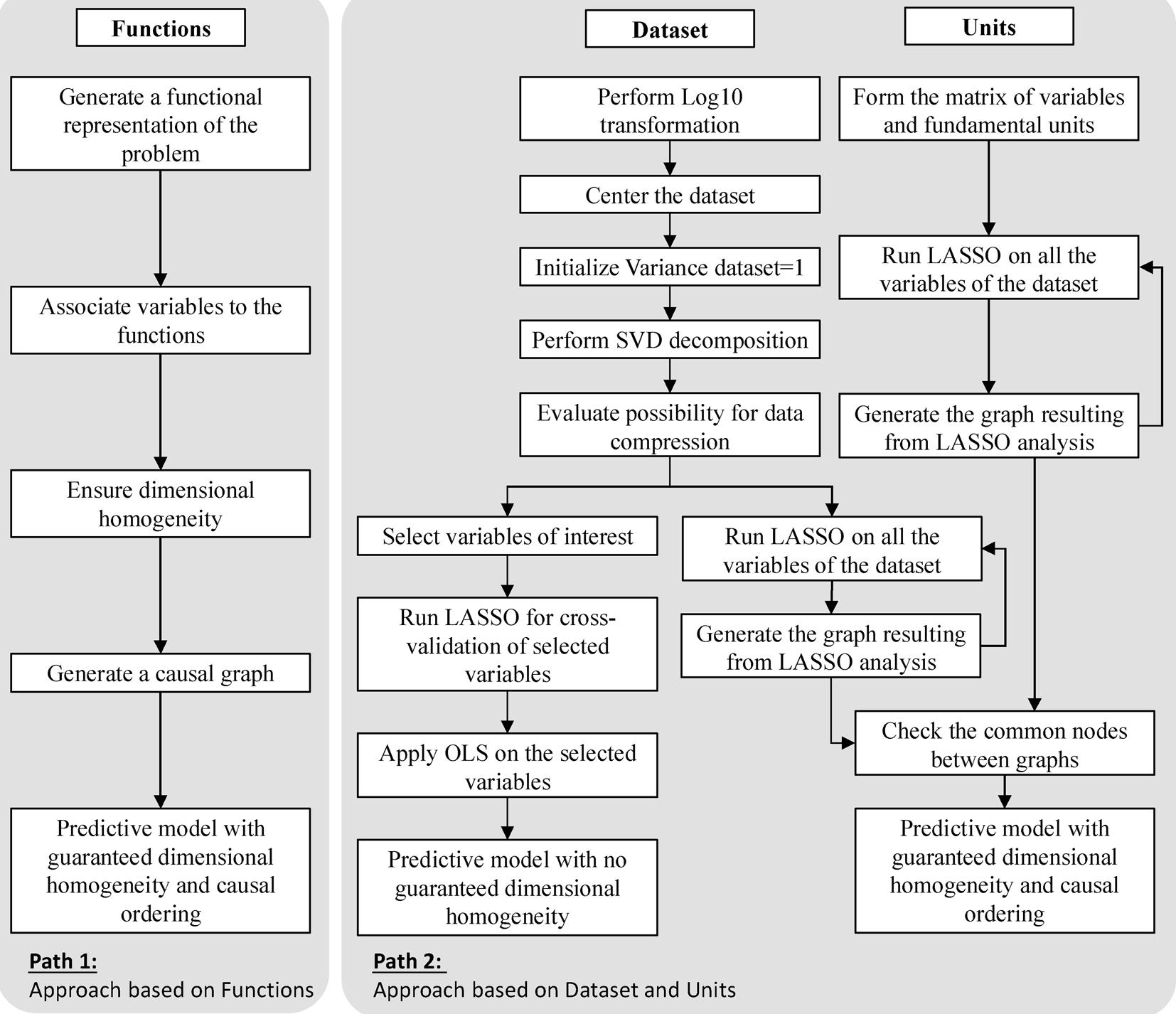
Fig. 2. General processes in DACM. Path based on functions and path 2 based on dataset and units.
The DACM framework is a modeling approach developed by the authors to produce models combining causally ordered graphs and power laws. In its functional-based usage, the DACM framework uses functional modeling combined with an algorithm-derived bond graph organs to create a causally ordered graph of a system associated with equations in form of power laws. It can also support the automatic search for physical contradictions as defined in TRIZ (Jordan, Reference Jordan1973; Savransky, Reference Savransky2000). In the functional part of the DACM theory, multiplicative relationships are used for all the modeling organs except between junctions (i.e., interfaces) where additive relationships are used.
Power laws can also be used to study natural phenomena in the form of probability distributions of variables. This is exemplified in the Bayesian usage of DACM in Figure 4. The overarching goal of this research is to provide a methodology for creating knowledge models combining the structure of causally ordered graphs and power laws. The sources of knowledge are dataset itself and the units of this dataset.
To do so, we need to measure and evaluate the semantic fidelity of simulation models as well as producing parsimonious and explainable models because those models are used later to reason and to propagate qualitative objectives. Non-causally ordered models may generate wrong predictions using this qualitative approach (Mokhtarian et al., Reference Mokhtarian, Coatanéa and Paris2017) and should consequently be avoided. Subsequently, the proposed modeling method can be viewed as a machine learning approach to develop integrated models with different levels of fidelity.
Figure 2 presents two separate modeling processes separated in two distinct paths, where path 2 is the focus of this paper. Additionally, Figure 3 summarizes possible usages of the resulting models that may help the readers to envision the potential applications of the research work presented in this article. The result of both paths 1 and 2 processes is a model combining an oriented graph and a set of power laws equations. In the case of path 2, two distinct models are produced using the approach presented in this work. One is a model produced using exclusively the information from the dataset but is not guaranteed to be dimensionally homogeneous. The other is a model formed of a causally oriented graph and power laws and is dimensionally homogeneous.

Fig. 3. Nature of the resulting models formed of a combination of an oriented graph and a power-law equation. The other predictive model with no guaranteed homogeneity does not differ in nature.
The implement of the method to generate models from dataset and its unit (i.e., path 2 shown in Fig. 2) is described step-by-step as follows. When working with generating power laws from dataset, it is practical to transform the initial dataset in order to ensure working with a linearized form. This is done by using the log10 transformations during the modeling process. The linear transformation allows using a large set of mathematical methods derived from linear algebra. The log10 transformation plays another role in the normalization phase that it allows reducing the scales of the different variables, thus, increasing the efficiency of the variable selection approach from data (i.e., the LASSO method which is an L1 regularization method). After the log10 transformation, the dataset is centered. This is followed by two classical operation in the process of preparing datasets, first centering the distribution and second obtaining a normalized variance of 1 for each column of the dataset (Freedman et al., Reference Freedman, Pisani and Purves2007). This is leading to the matrix presented in Appendix C (Variance analysis). This is useful especially when the numerical values associated with the variables exist in different order of magnitudes. After normalization, the method is followed by matrix decomposition, L1 regularization (i.e., LASSO), and L2 regularization (i.e., OLS) methods to enable complex system modeling. A more detailed account of the L1 and L2 regularization can be found in these publications (Xu et al., Reference Xu, Caramanis and Mannor2011; Pennington et al., Reference Pennington, Socher and Manning2014).
The matrix decomposition phase is using an SVD decomposition (i.e., an orthogonal decomposition ensuring that principal components are decoupled). The aim of the decomposition is to assess the potential benefit of a dimension reduction that could reduce the noise in the dataset and verify the validity of the hypothesis leading to the choice of the modeling in form of power laws. When this analysis is done, two actions are performed separately, first exploring the left branch of the path 2 process in Figure 2. LASSO is applied to select variables influencing the outputs of interest and the final regression using an OLS regression is applied to the set of influencing variables previously selected using LASSO. This process is leading to a model useful for making numerical predictions but not qualified for causal reasoning.
The right branch of the fork in path 2 is combined with the unit branch from path 2 and this combination is exploring the integration of the knowledge coming from the dataset and the fundamental units of the variables in the dataset to guarantee the dimensional homogeneity for the final model. This is done via a recursive use of LASSO on both the normalized dataset from Appendix C (Variance analysis and their fundamental units). The exploitation of Table 3 (the fundamental set of dimensions) in the case study is bringing several interesting properties such as sparsity, bringing stability of Table 3 to the LASSO selection process. As a result of the case study, two graphs are produced separately on the dataset and the dimensional unit's matrix of the variables in the case study in Figures 9 and 11. Those graphs are combined by retaining the common edges between graphs (i.e., shared connections between variables). This is allowing to generate a causally ordered graph integrating the additional knowledge source of the dimensional analysis.
Figure 3 presents an elementary exemplification of the final model produced by the DACM approach using the example of Newton's second law of motion. This law can be rediscovered using the approach described in path 2 of Figure 2.
The possible usages of such type of models are briefly summarized in Figure 4. The key purpose is to support synthesis and generation of novel solutions. The first usage is a qualitative usage. Using the mathematical machinery created by Bhaskar and Nigam (Reference Bhaskar and Nigam1990), it is possible to propagate backward the red objective in Figure 4 to find the green objectives that are resulting in our case from the positive exponents in the power-law relation F = m 1·a 1. This mechanism allows propagation in complex graphs and possible detection of physical contradictions (Savransky, Reference Savransky2000) appearing on individual nodes. It is possible using the TRIZ separation principle as well as other principles to reduce the contradictions. This is leading in the DACM framework to a modification of the graphs corresponding to a modification of the design and behavior of the designed system.
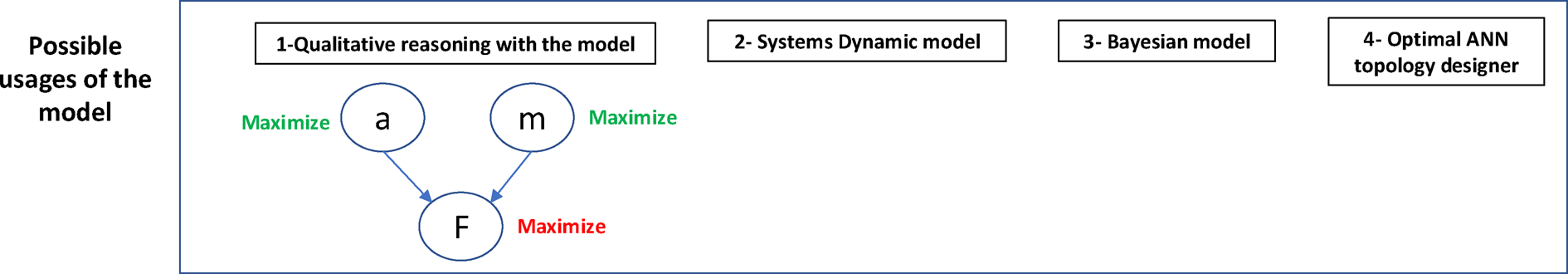
Fig. 4. List of possible design usages of the model produced.
The second usage of the graphs is a direct application of the model in the system dynamics framework (Sterman, Reference Sterman2001). The concept of stock and flow are not used but replaced directly by the variables of the model. The equations associated with the graph in Figure 3 are directly used to populate the system dynamics model. A third application is a direct usage as a Bayesian Network (BN) (Pearl, Reference Pearl2000). The training of the probability distributions in the BN uses the produced equation too. The topology of the BN is a direct result of the causal ordering from the DACM approach. Another related application is to use the DACM approach as a tool for optimizing the topology of artificial neural networks (ANNs). The equations produced in DACM can be used to generate a dataset itself employ to the train the ANN using a traditional supervised learning approach (Nagarajan et al., Reference Nagarajan, Mokhtarian, Jafarian, Dimassi, Bakrani-Balani, Hamedi, Coatanéa, Gary Wang and Haapala2018). The next section presents via a case study the path 2 from Figure 2. An initial analysis of the dataset is also done using a functional modeling perspective. This is allowing to reason about the transferability of the dataset to the desired case study. The message is that it is possible under certain conditions to use a dataset for design case slightly different from its initial production context.
Case study
Let us consider a physical phenomenon in which a stationary solid body is placed in a moving fluid. A drag force (w) is exerted on the sphere of diameter (l) due to friction generated by the moving fluid having the following characteristics of density (ρ), viscosity (ν), and velocity (V). The nonlinear physical phenomenon is illustrated in Figure 5.

Fig. 5. Pictorial representation of a stationary solid spherical body in a moving fluid.
The case study example is a classical problem in fluid dynamics in which the drag force resulting from the velocity of the flow of a certain fluid must be evaluated and modeled. In the example, the solid body is stationary whereas the fluid is in motion. To aid in the modeling and to facilitate the fidelity analysis, we can envision the case study example in the form of a product design case study. From a design context, the data regarding the variables of the system can be used to derive a design case study wherein, the solid body can be envisioned as a spherical underwater drone moving in seawater. The key difference with the initial case study description is that the drone (or solid body) is in motion with a velocity V and not the seawater (or fluid).
The underwater drone represented by the sphere of diameter (l) has a key function which is to navigate in the seawater. This movement is a source of friction due to the contact between the drone and seawater. Thus, from a system view, the desired function to move into the water can be defined, while an undesired function provided by the water can be defined to resist the movement of the drone. Using a taxonomy of functions presented in the DACM framework, a functional model of the original case study and the derived case study is presented in Figure 6. In both situations, the functions and their interaction remain the same.

Fig. 6. Functional representation of the case study in its original form (top) and derived form (down).
For the derived case study, the environment is made up of seawater with fundamental properties such as the density of the fluid (ρ) and the viscosity of the fluid (ν). The design objective for the drone would be to reduce the drag force (w) to facilitate the movement within the environment medium (seawater). By reducing the drag force, the energy consumption and maneuverability of the drone can be improved. The model to be created should use the experimental data collected (Appendix A) to derive relationships between the different variables of the system to compute the drag force as a function of different variables as presented in Eq. (1). It should be noted from the dataset (Appendix A) and Figure 6 that a unique dataset can be used to model two radically different engineering situations. In the original case study where the fluid is moving around a solid body while in the derived case study, a drone is traversing through a stationary seawater medium. Nevertheless, in both cases, the variables of the system and its environment remain the same, the difference is in the functional representation. From the perspective of fidelity, it is important to ensure that we would be able to differentiate between the two cases since they have different intended uses. Even though the model structure may appear similar, the individual variables are associated with different functions and parts of the system. Such a distinction is supported by the DACM framework by integrating a generic taxonomy of the variables (Mokhtarian et al., Reference Mokhtarian, Coatanéa and Paris2017). In DACM, the variables are classified as power variables and state variables. Power variables are decomposed into generalized flow and effort variables representing connections between different functions. Alternately, state variables are decomposed into generalized displacement, momentum, and connecting variables within a function. Using the variables of the system from the case study dataset (Appendix A), the functional representation of the derived case (Fig. 2) can be modified as shown in Figure 7. This dataset is a dataset produced by Prandtl and his team (Prandtl et al., Reference Prandtl, Wieselsberger and Betz1927) and used as it is for this article.

Fig. 7. Updated functional representation of the derived case study underwater drone moving in seawater.
Figure 7 can be presented mathematically [Eqs (1) and (2)] to show the behavior of each technical function described using verbs of action, to move, and to resist.
 $$V = f\;( {w, \;\rho , \;\nu , \;l} ), $$
 $$w = f\;( {V, \;\rho , \;\nu , \;l} ), $$
where V is the output of the desired function “to move” and w is the output of the non-desired function “to resist”. Using Eqs (1) and (2) and Appendix A, supplementary knowledge can be extracted about the fundamental dimensions (mass, length, and time) of the variables of the system. The variables of the system represented in the form of their fundamental dimensions are shown in Table 1. The encoding of the table is done in the following manner. For example, if the density ρ is considered, then its unit is in kg/m3. kg is a unit mass (M), and m is a unit of length (L). The exponent for kg is 1 and since kg is divided by m3, the exponent for m is −3. This is explaining the second columns of Table 1. The rest of the columns are constructed using a similar approach. For the last column, the force w measured in Newton (N), the reader should remember that a force, according to Newton's second law of motion, is a product of a mass (M) and an acceleration (L·T −2). As for w, the representation of variables using a combination of fundamental dimensions is also, for some variables, integrating the knowledge present in elementary laws of physics.
Table 1. Variables of the system represented in the form of fundamental dimensions

From Table 1, no columns are a linear combination of one another. The rank of the matrix in Table 1 corresponds to the maximal number of linearly independent columns of this matrix with a rank of five (5). Having three fundamental dimensions M, L, and T, it is possible to form 5–3 = 2 relations between the variables in the columns. Using the updated functional representation in Figure 7 and the dataset in Appendix A, a simulation model can be developed for the derived case study. The taxonomy developed in the DACM framework enables the clustering of variables and functions. A machine learning approach using the DACM framework is presented in this work to automate the generation of parsimonious models from datasets for the derived case study of the drone. First, the development of a simulation model from data is presented followed by an integration of dimensional homogeneity principles to measure and evaluate the fidelity of the developed model.
Modeling using power laws
The DACM framework was initially developed by the authors to generate oriented graph models for product-process modeling and metamodeling (Mokhtarian et al., Reference Mokhtarian, Coatanéa and Paris2017). The approach initially starts from a functional model which is used as the base upon which the oriented graphs are developed. The current article intends to move a step further to generate models directly from datasets to match current machine learning approaches for unsupervised and supervised learning applications (Pelleg and Moore, Reference Pelleg and Moore1999). The article leverage some key ideas, one of them, is to exploit the knowledge provided by the decomposition in form of fundamental dimensions presented in Table 1 as a supplementary knowledge complementing datasets and powered by the theory of dimensional analysis and the theorem of Vashy-Buckingham (Bhaskar and Nigam, Reference Bhaskar and Nigam1990; Szirtes, Reference Szirtes2007) presented in different forms in Eqs (3), (5), and (6) to detect potential confounders and to form valid causal ordering of the problem variables (Gilli, Reference Gilli1992). The final models produced by the approach presented in this article are in the form of a combination of oriented graphs associated with power laws (general form shown in Eq. (3)). The power laws provide a powerful tool to evaluate the dimensional homogeneity.
 $$Y = A\cdot X_1^{\alpha _1} \;\cdot X_2^{\alpha _2} \cdots X_n^{\alpha _n}, $$
where Y represents the output variable, A is a constant, Xi are the covariates, and α i represents the exponents of the covariates. The methodology developed in the article relies on classical tools from linear algebra facilitated by a normalization step using logarithmic transformation of the dataset. The log transformation proves advantageous for improving the efficiency of the different steps in the modeling approach. The normalization also aims at reducing the scale of the dataset using either a decimal or natural log transformation. However, it is important to ensure that the dataset does not contain negative or null values. Following the normalization procedure, the power-law expression in Eq. (3) can then be formulated as shown in Eq. (4).
 $${\rm log}\;Y = {\rm log\;}A + \alpha _1\cdot {\rm log}X_1 + \alpha _2\cdot {\rm log}X_2 + \cdots + \alpha _n\cdot {\rm log}X_n.$$
Subsequently, the equations for the model can be constructed in two ways as shown in Eqs (5) and (6). The knowledge extracted from the dataset in Appendix A is used to formulate Eq. (5) whereas, alternately, using the fundamental dimensions of the variable (shown in Table 1), the model can be formulated as Eq. (6).
 $$\pi _y = y_i\cdot x_j^{\alpha _{ij}} \cdot x_l^{\alpha _{il}} \cdot x_m^{\alpha _{im}}, $$
 $$\pi _y = [ D ] _i\cdot [ D ] _j^{\alpha _{ij}} \cdot [ D] _l^{\alpha _{il}} \cdot [ D ] _m^{\alpha _{im}}. $$
In Eq. (5), yi and xj,l,m represent the variables of interest. In Eq. (6), [D] represents the fundamental dimensions of the variables xj,l,m. In both equations, αi represents the exponents of the power law's form. The exponents in both equations can be similar or dissimilar depending on the nature of the source of information selected (i.e., the dataset or the fundamental dimensions). The exponents can be calculated directly from the experimental dataset, or the exponents can be calculated through dimensional analysis using the fundamental dimensions of the variables in the study. The fundamental dimensions are used in this research to improve the fidelity of the models produced as explained further in the section titled, Deriving a machine-learning model combining data and dimensions assources of information, starting with the analysis provided in Table 4. Thus, for the derived case study, two types of models can then be created using Eqs (5) and (6).
In the next subsection, the development of the simulation model directly from data is explained and demonstrated. The authors would like to highlight that the model developed in the next subsection uses only the experimental data and does not make use of the knowledge available regarding the dimension of the variables. Additionally, the clustering resulting from the use of the DACM taxonomy is not used in the next section. Instead, the DACM clustering is used as a cross-validation method to validate an automated clustering algorithm using LASSO directly from data.
Deriving a machine-learning model exploiting only the data source
In this section, a machine learning approach combining power laws and oriented graphs is presented to model the derived case study using the data from Appendix A. The modeling method follows the following steps namely, normalization of the dataset leading to the data in Appendix C, singular value decomposition (SVD), compression analysis, selection of the performance variables, selection of the variables influencing the performance variables, computation of the optimal relationships between selected parameters and performance parameters, and finally, the generation of the power models.
The normalization phase aims at linearizing the dataset to reduce the scale of the data but also to prepare the dataset for the use of linear algebra in the subsequent steps of the method. The SVD decomposition and compressibility analysis aim at applying compression, when possible, on the dataset to form a latent space. For many complex systems, the distribution of the principal components follows a long-tail distribution. Compression to the latent space can be beneficial for complex systems as it can remove noise in the signal and allow for a more efficient selection of important variables in the following data analytics phases. The compression to the latent space can be useful when the distribution of the variables is a long-tail distribution, otherwise, the compression step can be skipped.
The LASSO selection and its cross-validation are used to accurately select variables from the data which have a high influence on the performance variables thus, allowing for the development of parsimonious models. The performance variables are the variables selected by the modeler to assess the performance of the system.
The LASSO approach can be viewed as a variation of the OLS regression in which covariates not contributing to the output of the variables of interest are gradually discarded.
LASSO stands for Least Absolute Shrinkage and Selection Operator, in Eq. (8) below, the second term is the sum of the absolute value of the magnitude of exponents wj. A problem occurs since |w j| is not differentiable in 0. Updates of the coefficients w j are done in the following manner, when |w j| is becoming close to zero, a threshold condition is used to set w j to 0. The condition can be w j = 0 if |w j| < δ threshold.
LASSO provides sparse solutions. It is an excellent approach for modeling situations where the number of parameters to be analyzed is very high.
 $${\rm Min}\,\varepsilon ( w ) = \mathop \sum \limits_{i = 1}^n \displaystyle{1 \over {\sigma _i^2 }}\cdot ( {{\hat{y}}_i-y_i} ) ^2 + \lambda \mathop \sum \limits_{\,j = 0}^m \vert {w_j} \vert. $$
Thus, the approach works as a variable selection method contributing to the development of parsimonious models. Parsimony is an important principle in machine learning approaches due to their ability to support the generalization of models. LASSO acts as an L1-regularized regression method to support parsimony in the model development process but often at the cost of stability of the selection process. In the context of this paper, the stability of the selection algorithm can be seen as the method providing identical outputs on two datasets differing on only one sample value (Xu et al., Reference Xu, Caramanis and Mannor2011). Thus, to improve on the stability of the model development method, an L2-regularized regression (OLS) step is introduced to leverage the parsimony principle from LASSO but simultaneously improve the stability of the modeling approach.
The OLS regression phase brings stability to the model by providing an L2 regularization (i.e., computation of the optimal values of the coefficients in equations). The final power-law equations of the model are obtained by reversing the normalization steps.
The dataset follows the normalization approach presented in path 2 of Figure 2 and in the text above. The transformation of the dataset following the different steps in the modeling process is shown in Appendix B. The SVD is performed on the dataset after normalization at which point the variance of the dataset is equal to one (1). The goal of the SVD is to highlight the most important phenomena in the initial dataset and remove any secondary information or noise which is impertinent to the performance variables. The SVD decomposition for an input matrix [X] is shown in Eq. (8).
 $$[ X ] = [ U ] \cdot [ W ] \cdot [ V ] ^T.$$
Here, [X] is the input data matrix and [U], [W], and [V]T are the decomposed matrices resulting from the SVD. Following the SVD, the compressibility of the dataset is evaluated. Compression is possible if the decay of the eigenvalues of the input data matrix [X] follows a Pareto distribution. A Pareto distribution is a power-law distribution also called a long-tail distribution. Such distributions are often found in complex systems when hierarchy and subsystems are present. If such a distribution is not found, then LASSO variable selection is performed on a non-compressed dataset with the assumption that the noise or complexity of the dataset does not hinder the LASSO selection process. The compressibility check is performed by computing a linear fit (Fig. 8) for the decay of eigenvalues in the decomposed matrix [W] from Eq. (8). A log-log scale is used to ascertain the presence of a power law. An R-squared value computed for the fit can determine how well the regression fits with the observed data. A value closer to one (1) suggests that the regression fit matches well with the observed data and hence, can also suggest in our case the presence of power-law distribution (i.e., Pareto distribution).

Fig. 8. Linear fit for the decay of eigenvalues in log-log scale (vertical axis: eigenvalues and horizontal axis: singular values from first to fifth).
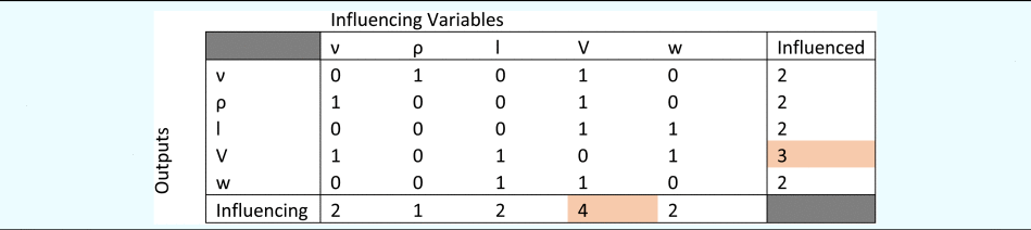
For the derived case study, the linear fit resulted in an R-squared value of 60.6% suggesting that the decay of eigenvalues does not follow a power-law (i.e., Pareto distribution). Thus, we can conclude that the benefit of applying compression to the current data set is limited or null. It can also be noticed that the design problem that we are studying is not integrating a hierarchy of subsystems at this level of analysis as reflected in the decay of Eigenvalues. This observation was verified using different compression levels during the LASSO selection parameter selection process explained further in the text. The compression appeared not to influence the LASSO process. Consequently, during the LASSO selection as well as the steps located after LASSO usage in path 2 of Figure 2, the dataset from Appendix C is exploited without compression. The result of the LASSO variable selection has been applied recursively to all the variables in the dataset is shown in Table 2.
Table 2. Variable selection using LASSO for the derived case study
It can be noted that the SVD decomposition and the linear fit for the decay of eigenvalues in log-log scale are also a measure of the conditioning of the dataset used in this article. This is impacting the numerical process and especially the matrix inversions and requires in specific cases to evaluate the number of digits required in the numerical process. Furthermore, sparse, well-structured, and well-conditioned matrixes are properties that are desired when processing matrixes (Kaveh, Reference Kaveh2018). The present article does not address those aspects but the exploitation of the dimensional analysis information from Table 1 has connections with those properties and is a practical way to use in addition of experimental datasets another source of information exhibiting those properties.
From Table 2, we can see that V, the speed of the underwater drone is shown to be the most influencing and influenced variable in the dataset. Thus, using Table 2, a graph-based representation is developed as shown in Figure 9 with V in the center.

Fig. 9. Graph-based representation of selected variables from LASSO for the derived case study.
Table 2 and Figure 9 will be reused for the fidelity analysis section of this article further. The LASSO selection is followed by the L2-regularized regression approach (i.e., traditional OLS) to model two outputs namely, V and w to represent performances of two key functions of the simulation model. Equations (9) and (10) show the general form in which the regression approach using OLS is computed.
 $${\log}\,V = {\log}\;A + \alpha _1\cdot \log \nu + \alpha _2\cdot \log l + \alpha _3\cdot \log w,$$
 $${\log}\;w = {\log}\;B + \beta _1.\log l + \beta _2.\log V,$$
Where log A and log B are the constants in the equation. Coefficients α i and β i are computed using the L2-regularized regression.
LASSO is an iterative approach wherein, a cut-off value for iterations must be specified to maximize the parsimony without reducing the precision of the model developed. The cut-off value for iterations is determined automatically at the point where the mean squared error (MSE) during selection starts to increase as shown for outputs V and w in Figure 10. The last values before having the MSE raising from 0 are selected so for V, the iteration 50 is selected and for w, the value 20 is selected in Figure 10.

Fig. 10. Iterations and their impact on the mean squared error (MSE) for output variable (V – top and w – bottom).
Following the OLS computation step, the final models for the output V and w with coefficients computed are shown in Eqs (11) and (12), respectively.
 $${\log}\;V = {-}0.039\cdot \log \nu -1.980\cdot \log l + 2.668\cdot \log w,$$
 $${\log}\;w = 0.747\cdot \log l + 0.370\cdot \log V.$$
The MSE for Eq. (11) was found to be 0.0039 with an R-square value of 0.996 and the adjusted R-square value of 0.9957. For Eq. (12), the MSE was found to be 7.46×10−04 with an R-square value of 0.999 and an adjusted R-square value of 0.999. The values suggest a very good fit to the observed data for both outputs. In both cases, the intercept values are null because of the normalization procedure performed in Appendix C. The final step in the model development method aims at converting Eqs (11) and (12) in the form of power laws. A denormalization approach is performed to enable the conversion. Equations (11) and (12) are first multiplied by the standard deviations for V and w, followed by adding to both equations the mean values for V and w. Finally, both equations must be exponentiated to obtain their respective power-law representation as shown in Eqs. (13) and (14) for outputs V and w, respectively.
 $$V = 7.328\cdot \nu ^{{-}0.01}\cdot l^{{-}0.57}\cdot w^{0.71},$$
 $$w = 0.107\cdot l^{1.032}\cdot V^{0.511}.$$
The computation of V and w for prediction purposes can be solved using a simple linear algebra method when the equations are in the linear format of Eqs (11) and (12), respectively. A simple algorithm is presented at the end of the section to ensure the computation of the unknown outputs for the derived case study.
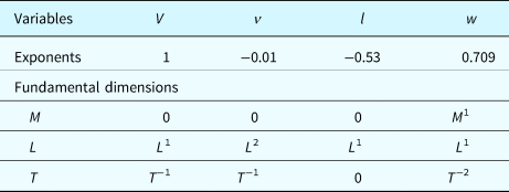
From Eqs (13) and (14), it is visible that both equations are not dimensionally homogeneous and cannot become dimensionally homogeneous even if a fundamental dimension is associated with the constants in the model as summarized in Table 3 for performance variable V.
Table 3. Dimensional homogeneity analysis for performance variable V in Eq. (13)
Deriving a machine-learning model combining data and dimensions as sources of information
From a fidelity perspective, a limitation of the models formed by Eqs (13) and (14) becomes apparent. The equations are not dimensionally homogeneous despite their usefulness for providing a good numerical prediction of the output variables. This is also a sign that the causality is not correct.
This can be due to the presence of confounding variables and relationships and/or from the incompleteness of the set of considered variables. Thus, this research further hypothesizes that integrating dimensional homogeneity can improve the fidelity of the developed models by supporting the detection of confounding variables and relationships. To do so, this research uses the DAT and Vashy-Buckingham theorem with the result of the LASSO analyses to improve the fidelity of the developed models. But first, we must tackle a fundamental problem faced by the DAT and the Vashy-Buckingham theorem. In the Vashy-Buckingham theorem, each Pi number produced [Eq. (5)] is the product of a performance variable and a subset of repeating variables. The Vashy-Buckingham theorem provides a necessary condition to create dimensionless numbers from a subset of variables. However, two problems not solved by the Vashy-Buckingham theorem remain: (1) How to select the performance variables meaningful to the study? and (2) How to build the associated subset of repeating variables, especially when multiple possible subsets are available? Figure 9 and Table 2 offer the start of an answer to both problems. From Table 2, we noticed that V is the variable having the most incoming edges and outgoing edges. From a DAT perspective, V is a desirable choice for a performance variable. In DAT, the problem is described using five variables and three fundamental dimensions. This is implying that two dimensionally homogeneous equations can be formed. Usually, two performance variables are selected to build those equations. Nevertheless, Figure 6 provides a useful piece of information. The speed V of the drone is provided first before getting feedback in form of a drag force w generated by the water. From Figure 6, it can be seen that the entire behavior of the system and the environment reaction described in the functional models are initiated by the speed V. w is then the consequence of V and one unique performance variable V can be considered in this case study. Figure 9 and Table 2 have been able to unveil this aspect automatically. Thus, the first question can be answered to determine the performance variable as highlighted using Table 2. The centrality measure in graph theory will allow to highlight such performance variables after producing Table 2 (Tutte, Reference Tutte2001). The authors would like to clarify that this result requires more extensive validation efforts using more case studies to be generalized. In our context, V is used as a performance variable for the two dimensionless equations that can be produced from the list of variables and their dimensions (i.e., five variables and three dimensions resulting in two equations). The next step is to select the appropriate repeating variables for which Figure 9 and Table 2 provide base knowledge. The performance variable must be connected with other repeating variables. Figure 9 can be used for this analysis but in its current state does not integrate any dimensional homogeneity principles. Thus, another iterative LASSO selection applied to the entire set of variables represented in the form of their fundamental dimensions from Table 3 is performed to create Table 4.
Table 4. Variable selection using LASSO for fundamental dimensions of variables in Table 1

The information from Table 4 is presented in the form of a graph in Figure 11. From the table and graph, choosing V as the unique performance variable, we have two directions in which we can move in Figure 11 to select the subset of repeating variables. The performance variable V with fundamental dimensions LT −1 has two DOFs, L and T. Thus, we would need to ensure that the choice of repeating variables can match the same dimensions of the performance variable (V). Moving up from speed (V) in Figure 11, the first choice of repeating variable would be the viscosity (ν). Following this, the length (l) would also need to be added to the first subset of repeating variables alongside viscosity (ν) to ensure dimensional homogeneity. Similarly, if we choose to move down from V in Figure 11, the first choice for repeating variable would be the drag force (w). However, the addition of drag force introduces another fundamental dimension which is mass (M) implying an additional DOF.

Fig. 11. Graph-based representation of variable selection from Table 4.
Thus, two more repeating variables namely density (ρ) and length (l) would be needed to ensure dimensional homogeneity in this case. For the performance variable (V), two dimensionless equations can be developed using the two different subsets of repeating variables as explained above. The method followed in this article provides an automatic mechanism to select the minimal subset of repeating variables required to ensure dimensional homogeneity. However, the authors would like to mention that the performance of the presented approach may be limited when several variables of the system contain the same dimensions and/or are a linear composition of other variables. In which case, the LASSO approach might randomly select one variable using the information available in Table 1. Thus, to ensure accurate selection of variables, a cross-validation approach is also included in the methodology by combining the results of Tables 2 and 4 as explained below. The idea is to provide a supplementary cross-validation mechanism to detect potential remaining confounders.
The cross-validation of the selection approach is performed by evaluating the shared similarity between Table 2 (selection based on data) and Table 4 (selection based on fundamental dimensions). By doing so, Table 5 can be developed which can validate the immediate connections for each variable.
Table 5. Cross-validation approach evaluating the shared similarity between LASSO selection results from Tables 2 and 4
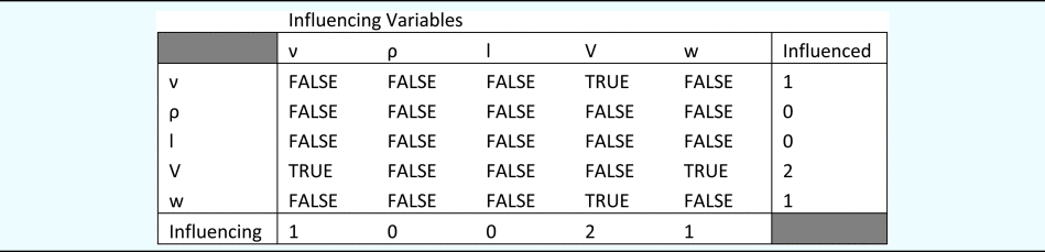
The “TRUE” values in the different cells in Table 5 implies that shared similarity was identified between the corresponding cells in Tables 2 and 4. Similarly, “FALSE” values imply a lack of shared similarity. Thus, for performance variable (V), the two choices for the first repeating variable would either be viscosity (ν) or drag force (w). Thus, Table 5 provides a validation of the LASSO selection results in Table 4. An alternate way to look at the connections determined by Table 4 and Figure 9 is that the direct link between ν → l in Figure 9, is established with the path ν → V → l in Figure 7. Similarly, the direct link between l → ρ in Figure 9, is established with the path l → V → ρ in Figure 7. Finally, the direct link between w → ρ in Figure 9 is associated with the path w → V → ρ in Figure 7 thus, providing the similarity of knowledge extracted directly from data and the fundamental dimensions of the variables in the data. In our case, it reinforces the confidence of the direct connections between variables provided by Figure 9, since it is cross-validated by indirect paths in Figure 7 through the intermediate node (V) in the graph.
Following the cross-validation of the variable selection process, we can develop the two dimensionless equations (i.e., 5 variables − 3 dimensions = 2 equations) for performance variable (V) using the two subsets of repeating variables chosen. The first subset contains viscosity (ν) and length (l), while the second subset contains drag force (w), density (ρ), and length (l) as repeating variables. The fundamental dimensions of each subset of repeating variables identified are shown in Tables 6 and 7, respectively.
Table 6. Fundamental dimensions of the first subset of repeating variables

Table 7. Fundamental dimensions of the second subset of repeating variables

The two tables above allow the computation of the exponents α i for Eq. (8). Two identical approaches can be used to achieve this objective. The vectors of the performance variable V are named [A] and the vectors matrixes of the repeating variables are collected in [B]. The following general relationship exists between the matrixes [Eq. (15)].
 $$[ A ] = [ B ] \cdot [ \alpha ], $$
where [α] represents the unknown coefficients ensuring the dimensional homogeneity which can be computed using Eq. (16).
 $$[ \alpha ] = [ B ] ^{{-}1\ast }\cdot [ A ], $$
where [B]−1* represents the Moore-Penrose pseudoinverse. The use of pseudoinverse is required since matrix B is not always a square matrix. The pseudoinverse is calculated as shown in Eq. (17).
 $$[ B ] ^{{-}1\ast } = ( {{[ B ] }^T[ B ] } ) ^{{-}1}\cdot [ B ] ^T.$$
The calculation of the [α] using the Moore-Penrose pseudoinverse can also be substituted by OLS regression to obtain the coefficient values. Thus, from the vector and matrix representations in Tables 6 and 7 and using Eqs. (15)–(17), the two dimensionless equations for performance variable (V) are shown in Eqs (18) and (19), respectively.
 $$V = \pi _{\rm Re}\cdot \nu ^1\cdot l^{{-}1},$$
 $$V = \pi _{\rm Cd}\cdot w^{1/2}\cdot \rho ^{{-}1/2}\cdot l^{{-}1}.$$
Both equations can be rearranged in the following form [Eqs (20) and (21)] in which π Re and π Cd are two dimensionless values resulting from the ratio of the variables in Eqs (18) and (19), respectively. From the perspective of fluid dynamics for the derived case study, π Re represents the Reynolds number (Re) commonly used to predict flow patterns. The second one is the drag coefficient, also a dimensionless value used to quantify the resistance of an object in a fluid environment.
 $$\pi _{\rm Re} = \displaystyle{{Vl} \over \nu },$$
 $$\pi _{\rm Cd} = \displaystyle{w \over {\rho V^2l^2}}.$$
From Eqs (20) and (21), we have four variables which are unknowns namely, V, w (original outputs of the derived case study as shown in Eqs (13) and (14)), π Re, and π Cd (the dimensionless numbers developed in Eqs (20) and (21)). Thus, Eqs (13), (14), (20), and (21) must be computed conjointly to solve the system of equations. The initial modeling objective in this article for the derived case study aimed at modeling the speed (V) and drag force (w) which can be accurately predicted with the parsimonious models developed in Eqs (13) and (14). However, Eqs (20) and (21) developed using DAT overlay an additional layer of information to the model. Evaluating in the context of the functional model developed for the derived case study, Eqs (13) and (14) only assess one parameter in each function of the drone. However, the second set of models was developed using DAT in Eqs (20) and (21) assess globally each of the functions of the drone shown in Figure 4. The current representation in Eqs (20) and (21) provide a dimensionally homogeneous expression fulfilling the required specification of a function thus, suggesting a higher level of fidelity in the developed approach.
The two sets of models [Eqs (13) and (14), and Eqs (20) and (21)] can be represented graphically (Fig. 10) to holistically represent the model. In Figure 10, arrows represent the connection between variables.
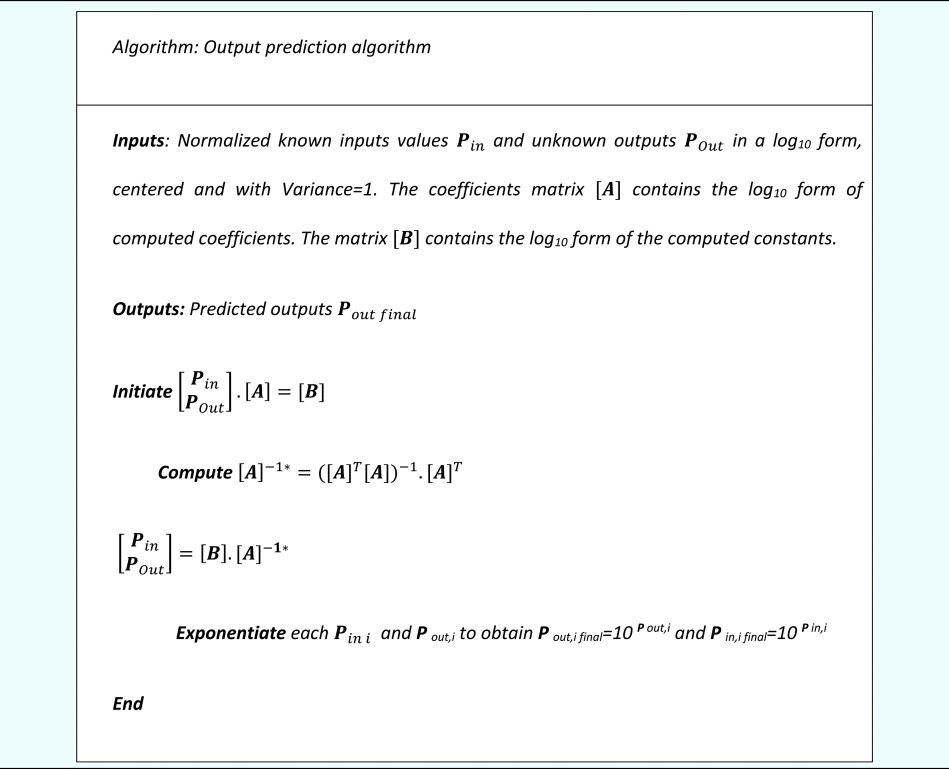
Solid arrows represent the lower fidelity connections of the system model where fitting using data and parsimony criteria are fulfilled. The dotted arrows combine the fitting and parsimony criteria but in addition, integrate dimensional homogeneity to enable a causal ordering. The graph-based model shown in Figure 10 can be used as a pretrained topology for an ANN model. The prediction of the unknown outputs V, w, π Re π Cd in Figure 10 is done using the algorithm presented in Tables 6 and 7. The algorithm is generic and can be applied to all problems analyzed using this approach. Figure 12 associated with Eqs (13), (14), (20), and (21) is a specific type of ANN. This type of ANN differs from traditional ANN due to the topology design of the structure of the oriented graph. It differs also in the way the training of the weights is done and in the nature of the equations governing the modeled phenomena. The algorithm for computing unknown output is presented in Table 8.

Fig. 12. Final oriented graph model for the derived case study showing two levels of fidelity (1 – lower fidelity, variable level: yellow; and 2 – higher fidelity, function level: gray).
Table 8. Algorithm for computing the unknown outputs for the derived case study
The graph model (Fig. 10) can also be used to define a BN topology wherein, the equations can be used to determine the conditional relations between different variables (represented as nodes in a BN) to facilitate the Bayesian inference mechanism. The final graph model produced in this section integrates two levels of fidelity. The first level facilitates computation at the variable level and is not dimensionally homogeneous. The second level provides the required granularity to holistically assess a function's performance and behavior concerning the system of interest. Additionally, this second level of fidelity also ensures dimensional homogeneity as well as a valid causal ordering compliant with modeler expected usage of the model. Those aspects will be studied further in future studies. Selection of the variables influencing the performance variables, computation of the optimal relationships between selected parameters and performance parameters, and finally, the generation of the power models.
Discussion and future work
This research presented a modeling and machine learning method to create simulation models with measurable levels of fidelity for engineering design. The method is a machine learning method serving as a basis for evaluating the fidelity of different types of models. The developed approach generates parsimonious explainable models that enable generic knowledge representation in the form of oriented graph with valid causal ordering, associated with power laws. The approach uses data as initial knowledge to model the system using power laws and graph-based representations of the modeled equations. The graph-based representation is a synthetic manner of representing the different equations increasing the interpretability of the model. The research also highlights the use of the graph-based representation as a precursor to generating the graph topology for more classical machine learning approaches such as BNs and ANNs. The graph representation used in this work is an approach to create optimal topologies for BN and ANNs as well as training the specific form of ANN presented in this work.
From the viewpoint of model fidelity, the developed method demonstrated the existence of different levels and sources of knowledge (i.e., the experimental dataset and the dimensions of the variables). The models produced using the two sources of knowledge are different and provide two levels of granularity in the demonstrated case study. The first level of granularity was at a variable level to predict the key performance parameters of the derived case study presented in Figure 3. The second level of granularity is achieved for the computation of system-level criteria, the key functions (desired and non-desired) of the system of interest for the derived case study. The two levels of granularity in the developed model can be associated as two intricated layers of fidelity, an initial layer, with a lower fidelity and not adhering to the dimensional homogeneity criteria, and a second level matching the homogeneity criteria. Together, the two levels of the model can be represented in form of a synthetic graph. A part of this graph is an oriented graph representing the first layer of fidelity, while the second part is an oriented graph with a validated causal ordering representing the second layer of fidelity. This causal ordering is compliant with the intentional use of the model by the modeler as presented in the background section.
The developed method can be coined as a machine learning method for its ability to automatically model the system based on experimental data. In addition, the method enables simulations using the graph presentation and the output computing algorithm (Table 8) presented in the paper. The developed approach will be applied in future work to the dynamic control of manufacturing systems. One requirement for such an application is the need for the control system to be able to respond to sensors information in close to real-time. The parsimonious nature of the models developed using this method can offer the benefit to be light and can be integrated into decentralized control systems located as close as possible from sensors. Additionally, an interesting characteristic of the developed method is the composability of the models providing a modular approach where elementary building blocks can be assembled to form extended models.
The research developed in this article presents a novel combination of known and validated methods to generate an actionable framework contributing to the fidelity evaluation of models. Tangible criteria relying on dimensional analysis and their interrelations with the concept of variables and functions have been leveraged in the developed modeling approach to represent two specific levels of fidelity. Additionally, this supplementary knowledge was used to direct the causal ordering of the second model. It is claimed that a direct link exists between a higher fidelity and a valid causal ordering. It was also demonstrated that the higher fidelity model was corresponding to a representation of the behavior of functions of the studied system. The developed approach demonstrates that simulation at lower granularity level (i.e., variable level) can be performed efficiently with a lower model fidelity while function level models requires a higher model fidelity, at least for the case study exemplified in this research. Higher fidelity in the models can be achieved by using the supplementary knowledge provided by the fundamental dimensions of the variables. The analysis presented in this research has voluntarily been focused on engineering models.
The key contributions of the research are highlighted as follows:
1) A machine learning approach for engineering modeling using data, for generating parsimonious and explainable models has been presented. A cut-off criterion is defined to combine the parsimony and precision of the model. The different steps of the machine learning method have been exemplified in the case study.
2) It has been shown that the LASSO graphs resulting from an experimental dataset and a supplementary information in form of a dimensional dataset (i.e., Table 1) can be used as a cross-validation method for the selection of the variables forming the performance and repeating variables in the higher fidelity model. This contribution is effective in the exemplified case in this research but needs to be validated further for other complex case studies.
3) Two interrelated models have been developed and aggregated via a graph-based representation. Obtaining the highest level of fidelity implies the fulfillment of supplementary constraints requiring a holistic set of variables related to the different functions of a system. The research enables modeling at distinct levels of fidelity, integrated into a single graph-based model which supports simulation.
4) Finally, an algorithm for predicting the unknown outputs for the distinct levels of fidelity in the models has been presented as a new form of ANNs.
The method developed in this article can be viewed as a reverse engineering approach capable of extracting explainable knowledge in a parsimonious form from diverse types of collected datasets. The log transformation used in the dataset normalization enables the use of linear algebra algorithms to analyze highly nonlinear problems. The modeling method combines conjointly L1 and L2 normalization to support the optimal selection between parsimony and stability in the models produced. The developed approach is computationally efficient and is scalable for larger datasets. In the current research, the size of the datasets handled by the method is potentially small. In this respect, the method demonstrates that efficient modeling of problems where data are very limited can be performed. Like human learning, only a small number of experiments are requested for new learnings.
The idea underlying the paper is to propose a method coming closer from the number of cases required by the human learning process. Samples of the size of two digits in our case can be considered as small. Small dataset is associated with poor statistical validity of the models produced. Therefore, we need to exploit other sources of knowledge not directly present in the dataset. We exploited the units of the variables from the dataset. Those units allow us to generate sparse matrixes, well-conditioned matrixes and well-structures matrixes (Kaveh, Reference Kaveh2018) bringing stability to the algorithms together with the L2 regularization used by OLS regression. They can compensate for the limited size of the dataset and for the inability of the machine learning methods to integrate the dimensional analysis homogeneity.
A limitation of the current work not discussed in the paper, but of fundamental importance for the scope of the approach, is that metrics are not always available to measure variables in a dataset. Multiple situations in design, and social sciences exist where getting a measure metric for variables in a dataset is a challenge. The authors are developing an approach allowing the exploitation of linguistic definitions to generate the type of matrixes presented in Table 1. This development is a significant expansion of the scope of the work presented in the paper and significantly increase the application domain of the approach.
Future work will assess different case studies and problems where collinearity between variables exists. This is important to make the approach robust and validate the generic principles emerging from this study. Second, the presented approach has established a link between fidelity, the nature of the knowledge, and the nature of the models. Nevertheless, the concept of fidelity is broader, and a real operationalization of that concept needs to be associated with quantified tolerances. For operational use, it is important to define the minimal and maximal fidelity acceptable for a model. Additionally, it is important to be able to measure the fidelity of the model and to compare it with given tolerances. To do so, the authors plan to expand on the framework proposed to quantify fidelity by transforming criteria such as dimensional homogeneity, completeness of variables set, types of datasets, produced models into quantifiable and measurable criteria or levels.
Data availability statement
The data used in the article is reproduced at the end of the article in the appendix. This dataset was produced by Prandtl et al. (Reference Prandtl, Wieselsberger and Betz1927) and reused by the authors.
Financial statement
The research presented in this article was funded for H.N. by the DIGITBrain project from H2020 (EU commission) and for D.W. and S.P. by the Smaragdi project (Business Finland).
Conflict of interests
No competing interests related to the presented research exist for the authors of the article.
Dr. Eric Coatanéa received his BS degree in mechanical engineering in 1990 from the University of West Brittany, Brest, France, his MS in mechanical engineering from INSA Toulouse, France in1993, and his teaching certification from Ecole Normale Supérieure of Cachan, France in 1994. Dr. Coatanéa worked for 11 years as a teacher of manufacturing engineering at the University of West Brittany, Brest, France while in parallel being very active in track and field. He embarked in joint doctoral studies in 2002 and received his joint PhD degree in mechanical engineering from Helsinki University of Technology, Finland (nowadays Aalto University) and the University of West Brittany, Brest, France in 2005. Currently, Dr. Coatanéa is a Professor of Manufacturing Engineering and Systems Engineering at the Faculty of Engineering and Natural Sciences, Tampere University, Finland. He was Marie-Curie fellow in 2005–2007. He held several visiting professorships at different universities. Dr. Coatanéa is in charge of the Manufacturing research group at Tampere University. His research interests include design and manufacturing activities, system thinking, and system engineering. More specifically, the research focus is given to the early integration of simulations and decision support tools during the initial design phases.
Hari Nagarajan is a research scientist in advanced manufacturing technologies at the Technical Research Centre of Finland, VTT. He received his PhD in mechanical engineering from Tampere University (Finland) in 2022. His research interests include Life Cycle Engineering, Material Processing using Additive Manufacturing, Metamodelling Framework Development for Additive Manufacturing, and Sustainability Evaluation.
Hossein Mokhtarian is a University Lecturer at Tampere University. He holds a double PhD degree from Tampere University (Finland) and Grenoble Alpes University (France) in mechanical engineering and industrial engineering. His research interests include the intersection of digital design and advanced manufacturing. He has a passion and solid pedagogical background.
Di Wu is a post-doctoral researcher at Tampere University. He got his PhD degree from Simon Fraser University (Canada) in mechanical engineering. His research major is multi-disciplinary design optimization, machine learning/deep learning methods, and their applications in engineering designs.
Suraj Panicker is a doctoral researcher working at Tampere University, Finland. His research interests include metal additive manufacturing, sustainable manufacturing, and data analytics in manufacturing.
Andrés Morales-Forero is a PhD candidate in industrial engineering at Polytechnique Montreal, Canada. His research focuses on Causal Machine Learning and Safe, Ethical, and Explainable AI. He is currently working on different projects to find mathematical and statistical models for complex challenges in research, industry, and society.
Samuel Bassetto is a Canadian professor of industrial and system engineering at Polytechnique Montréal. He is born and made his scholarship in France. He earned PhD in 2005, from ParisTech – Arts et Métiers. He got his MSc in artificial intelligence from the University of Lorraine in 2001 and his BIng in mechanical engineering from ParisTech also in 2001. He worked for several industrial companies from 2001 to 2006. Since 2006 in the University of Savoie in France and in 2011 in Polytechnique Montréal in Canada. He has directed more than 100 MSc and PhD students, co-published more than 70 scientific papers, and earned several awards for his research. Now he directs the LABAC, his R&D laboratory of process control. He focuses the research on the design of intelligent alarms (data science and artificial intelligence) and relevant actions (psychiatry and neuroscience). He is also a caver and a climber.
Appendix A. Experimental data

Appendix B. Log10 transformation

Center the dataset

Appendix C. Variance analysis


 Open access