


1. Introduction
We consider a falling liquid film in contact with a laminar counter-current gas flow within a narrow rectangular channel inclined at an angle  $\beta$ (figure 1). This configuration can be considered as a prototype for compact devices found in engineering applications, such as reflux condensers and distillation columns with structured packings (Valluri et al. Reference Valluri, Matar, Hewitt and Mendes2005). It is well known that the interaction between the wavy film and the gas flow can promote flooding events leading to a deterioration in the process performance. Depending on the geometry and/or ratio of liquid and gas flow rates (or superficial velocities), we can observe film atomization (Zapke & Kröger Reference Zapke and Kröger2000), wave or liquid flow reversal (Tseluiko & Kalliadasis Reference Tseluiko and Kalliadasis2011) or obstruction of the channel (Vlachos et al. Reference Vlachos, Pars, Mouza and Karabelas2001). In order to prevent or delay such events, it is crucial to characterize the dynamics of interfacial waves and in particular their linear and nonlinear responses to the gas flow.

Figure 1. Sketch of the experimental set-up. The liquid loop appears in blue and the gas path is highlighted by a red arrows in the channel gap.
Many theoretical and experimental works dedicated to the linear stability of falling films are reported in the literature since the seminal work of Kapitza (Reference Kapitza1948) on the different wavy flow regimes. The linear stability analysis of a liquid film in a passive atmosphere was initiated by Benjamin (Reference Benjamin1957) and Yih (Reference Yih1963). They found that the film is unstable to long-wave disturbances when the Reynolds number is greater than  $5/6 \cot \beta$ through an inertia-driven mechanism. This threshold for the so-called Kapitza instability was confirmed experimentally by Liu, Paul & Gollub (Reference Liu, Paul and Gollub1993). Recent theoretical investigations (Lavalle et al. Reference Lavalle, Li, Mergui, Grenier and Dietze2019) have shown that the impact of the gas phase on the linear stability threshold becomes non-negligible in weakly inclined and/or strongly confined channels by causing a stabilizing effect and ultimately the full suppression of the Kapitza instability. This linear stabilization due to confinement was confirmed experimentally in Lavalle et al. (Reference Lavalle, Li, Mergui, Grenier and Dietze2019) for a water film in contact with quiescent air in a slightly inclined channel ( $\beta =1.69^{\circ }$) of height $H=5$ mm. The main ingredient involved in the stabilization mechanism was found to be the tangential viscous stress exerted by the gas on the film surface, as suggested by Tilley, Davis & Bankoff (Reference Tilley, Davis and Bankoff1994). The strong stabilizing effect induced by a counter-current air flow on a wavy water film is reproduced by Trifonov (Reference Trifonov2019) at small inclination and strong confinement. Kushnir et al. (Reference Kushnir, Barmak, Ullmannl and Brauner2021), via a comprehensive parametric study, have recently established that regimes of linear stabilization in the case of a zero net gas flow occur for channel heights $H \leqslant 10$ mm at $\beta =1^{\circ }$ and $H \leqslant 2$ mm at $\beta =10^{\circ }$ in a water–air system.
Furthermore, when the gas flows in a counter-current fashion, it was shown in Lavalle et al. (Reference Lavalle, Li, Mergui, Grenier and Dietze2019) that the linear stabilization is intensified over the entire range of unstable wavenumbers when the confinement is sufficiently strong. For intermediate confinement levels, the linear effect of the gas flow can become non-monotonic, i.e. the cutoff wavenumber of the Kapitza instability first decreases and then increases with the gas flow rate (Vellingiri, Tseluiko & Kalliadasis Reference Vellingiri, Tseluiko and Kalliadasis2015; Trifonov Reference Trifonov2017; Lavalle et al. Reference Lavalle, Li, Mergui, Grenier and Dietze2019). The stabilizing effect observed at low gas flow rate arises at all wavenumbers. By contrast, when the gas flow rate is large, short waves are attenuated while long waves are amplified, in accordance with the experiments of Alekseenko et al. (Reference Alekseenko, Aktershev, Cherdantsev, Kharlamov and Markovich2009) and Vellingiri et al. (Reference Vellingiri, Tseluiko and Kalliadasis2015) on linear waves in a vertically falling liquid film, which were conducted in a vertical tube with a turbulent counter-current gas flow. Finally, for weak confinement, a monotonic increase of the cutoff wavenumber is observed and the destabilization of the film arises at all wavenumbers.
The nonlinear response of surface waves has also been studied in a number of works, usually involving a turbulent counter-current gas flow in the context of flooding (Vlachos et al. Reference Vlachos, Pars, Mouza and Karabelas2001; Drosos, Paras & Karabelas Reference Drosos, Paras and Karabelas2006; Trifonov Reference Trifonov2010; Tseluiko & Kalliadasis Reference Tseluiko and Kalliadasis2011; Kofman, Mergui & Ruyer-Quil Reference Kofman, Mergui and Ruyer-Quil2017). These studies, which concerned weak confinement levels or vertical configurations, revealed that the amplitude of nonlinear waves increases and steepens with increasing gas flow rate while their speed decreases. The authors also observed that capillary ripples in front of the solitary waves are damped, in line with the linear stabilization of short waves observed by Alekseenko et al. (Reference Alekseenko, Aktershev, Cherdantsev, Kharlamov and Markovich2009). In the weakly confined setting, flooding manifests itself in experiments as wave reversal or wave breaking phenomena (Drosos et al. Reference Drosos, Paras and Karabelas2006; Kofman et al. Reference Kofman, Mergui and Ruyer-Quil2017) emerging from the interfacial shear stress imposed by the gas flow. By contrast, in strongly confined vertical channels, flooding is usually associated with a wave-induced local obstruction of the channel cross-section (Vlachos et al. Reference Vlachos, Pars, Mouza and Karabelas2001; Dietze & Ruyer-Quil Reference Dietze and Ruyer-Quil2013), which can coincide with wave reversal events (Lavalle et al. Reference Lavalle, Grenier, Mergui and Dietze2020). In such configurations, the counter-current gas flow amplifies the wave height and thus increases the flooding risk. Recent numerical investigations suggest that this trend could be inverted in weakly inclined channels. For example, Trifonov (Reference Trifonov2019) identified a non-monotonic variation of the interfacial velocity, mean film thickness and interphase friction coefficient with increasing counter-current gas velocity, although the trend of the wave amplitude remained monotonic and increasing. Lavalle et al. (Reference Lavalle, Mergui, Grenier and Dietze2021) have identified regimes where the nonlinear wave height and the linear growth rate both decrease with increasing gas flow rate. Such regimes, if confirmed experimentally, could avoid catastrophic flooding events, while exploiting the benefits of surface waves (e.g. intensification of heat and mass transfer).
The main aim of the current manuscript is to confirm the existence of such regimes through experiments. We study the effect of a counter-current laminar air flow on forced two-dimensional (2-D) solitary waves resulting from the Kapitza instability in a weakly inclined ( $\beta = 4.9^{\circ }$) strongly confined channel of $5$ mm height. A particular attention has been paid to the boundary conditions, specifically designed to avoid flooding due to outlet effects at the end of the test section, thus allowing us to focus on the wave dynamics in the core of the channel. Temporal forcing is applied at the liquid inlet to force surface waves within a buffer zone before they come into contact with the air flow. The influence of the gas shear stress on the shape, amplitude and velocity of these nonlinear waves is investigated and contrasted with the experiments of Kofman et al. (Reference Kofman, Mergui and Ruyer-Quil2017), which were performed in a weakly confined channel ( $H=19$ mm) where the gas flow was turbulent. Furthermore, we are interested in the effect of the surface waves on the mean film thickness when the gas velocity is increased.
The paper is organized as follows. The experimental set-up and the measuring techniques are presented in § 2. Results are presented in § 3, where we discuss the response of nonlinear surface waves to an increase in counter-current gas flow rate. In § 3.1, we focus on the role of the confinement level, by contrasting our results with the weakly confined experiments of Kofman et al. (Reference Kofman, Mergui and Ruyer-Quil2017). In § 3.2, we focus on the effect of the counter-current gas flow on the dynamics of precursory capillary ripples. In § 3.3, we discuss the role of the liquid Reynolds number and finally in § 3.4 we assess the effect of surface waves on the mean film thickness. Conclusions are drawn in § 4.
2. Experimental set-up and measurement methods
A general view of the experimental apparatus is sketched in figure 1: a liquid film falling on the bottom plate of an inclined rectangular channel in contact with a counter-current gas flow. Figure 2 displays a cross-sectional view of the channel. The liquid-related part is the same as the one used in Lavalle et al. (Reference Lavalle, Li, Mergui, Grenier and Dietze2019). In § 2.1, we recall briefly its main characteristics. Then in § 2.2 we describe the part related to the gas phase.
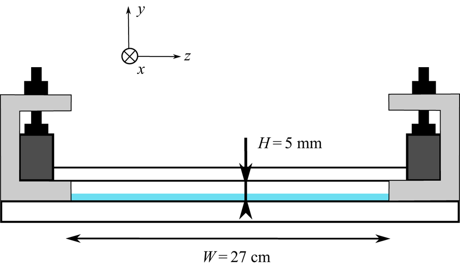
Figure 2. Sketch of the channel cross-section.
2.1. Liquid loop
The liquid-related part consists of an inclined glass plate ( $L=150$ cm long, $W=27$ cm wide and $5$ mm thick) placed on a massive framework mounted on rubber feet to dampen environmental vibrations. The inclination angle $\beta$ can be changed in the range $0^{\circ }\unicode{x2013}20^{\circ }$ and is measured using an inclinometer with a precision of $0.05^{\circ }$. In this work $\beta$ is fixed to $4.9^{\circ }$. At the channel exit, the glass plate is extended with a porous medium that drains the liquid away, allowing us to avoid flooding events due to exit effects. A gear pump brings the liquid from the outlet tank located at the exit of the plane to an inlet tank, from which the liquid overflows and runs onto the plane. The volumetric liquid flow rate, $q_l$, is changed by varying the pump power and is measured by using a magnetic-induced flow meter. The liquid Reynolds number is calculated as
 \begin{equation} \textit{Re}_l = \frac{q_l}{\nu_l W}, \end{equation}
where  $\nu _l$ is the kinematic viscosity of the liquid.
In this study,  $\textit {Re}_l$ is varied in the range 20–49. A temporal periodic forcing of the film is introduced at the inlet to trigger surface waves of prescribed frequency $f$. This is achieved through a thin aluminium plate fixed to the membrane of two loudspeakers thus generating harmonic vibrations above the liquid surface across the whole width of the inlet tank (Kofman et al. Reference Kofman, Mergui and Ruyer-Quil2017). The choice of the forcing frequency depends on $\textit {Re}_l$ and is based on the aerostatic case (without counter-current gas flow). We adjust it such that 2-D saturated travelling waves are observed at the end of the unsheared zone while avoiding secondary subharmonic or side-band instability (Liu & Gollub Reference Liu and Gollub1994). The waves then form a regular wave train over the working area and appear as a large hump preceded by capillary ripples.
Water is used as working liquid. The temperature of the liquid is measured in the outlet tank and upstream of the inlet tank. The surface tension is regularly monitored by taking a water sample then using a drop shape analyser. A one-point temporal measurement of the film thickness based on the confocal chromatic imaging (CCI) technique (Cohen-Sabban, Gaillard-Groleas & Crepin Reference Cohen-Sabban, Gaillard-Groleas and Crepin2001) is performed through the bottom glass plate with a spatial precision of  $250$ nm and a temporal resolution up to $2$ kHz. The CCI probe is mounted on a linear translation stage in order to perform measurements along the streamwise axis of the glass plate. In this study, the film thickness is measured at the midwidth and at $x=60$ cm from the inlet (see figure 1). An example of a CCI time trace is shown in figure 3(a). From such temporal measurements, we can extract the time-averaged film thickness, $h_m$ (blue line) and the film thickness range, given by $h_{max}$ and $h_{min}$, which correspond to the statistical mean of the maximum and minimum wave height values measured over the duration of the signal (red line and green line). The temporal fluctuations of $h_{max}$ and $h_{min}$ are quantified from the standard deviation of the statistical measurements and are used to include error bars in the relevant figures.

Figure 3. Film thickness time trace measured with the CCI technique. Here  $\textit {Re}_l=35$, $f=2.8$ Hz, $\eta _0=11.1$, without counter-current gas flow. (a) The blue line corresponds to the time-averaged film thickness over the duration of the signal. Open and filled circles correspond to the minimal and maximal height of each wave in the signal, respectively. (b) Enlargement of the signal presented in (a). Squares and downward triangles mark the maximum positive free-surface slope magnitude, located at the back of the first capillary wave and at the main wave tail. Upward triangles mark the maximum negative free-surface slope magnitude, located at the main wavefront.
In addition, we can extract the local free-surface temporal slope,  $\partial _t h$, and calculate the statistical mean of its maximum and minimum values over the duration of the signal, as well as the related standard deviation. Figure 3(b) represents a blown-up view over three wave periods, where we have highlighted the maximum (positive) and minimum (negative) free-surface slope magnitude, located at the back of the first capillary wave (square) and at the main front (upward triangle), respectively. The maximum free-surface slope magnitude is also indicated (downward triangle).
For a given liquid Reynolds number, we quantify the relative confinement of the liquid film with the global parameter
 \begin{equation} \eta_0 = \frac{H}{h^{0}_m}, \end{equation}
where  $h_{m}^0$ is the time-averaged film thickness measured in the case of a quiescent gas (superscript 0), i.e. without imposing a counter-current gas flow.
In addition to the pointwise CCI film thickness measurement, we visualize the film surface with shadowgraphy. For this, the film is illuminated with an oblique white light sheet and imaged from the top either by a 2-D camera to provide shadowgraphs over whole width and length of the working area (figure 4a) or by a linear CCD camera focused on the central axis ( $z=0.5W$) to obtain spatiotemporal diagrams (figure 4b) from which the wave speed, $c$, is determined. At least two spatiotemporal diagrams are acquired for each experiment and we measure the velocity of several waves around $x=60$ cm on each diagram. Then $c$ is the mean of the set of measurements and the related error is given by corresponding the standard deviation. The wave speed can also be used to convert the temporal slope $\partial _t h$ of the film surface to the spatial slope $\partial _x h=\partial _th/c$.

Figure 4. Typical experiment:  $\textit {Re}_l=35$, $f=2.8$ Hz, $\eta _0=11.1$, without counter-current gas flow (aerostatic case). (a) Visualization of the gas–liquid interface over the entire test section. The white arrow marks the length over which spatiotemporal diagrams are constructed. The filled white circle marks the location for the CCI measurements ( $x=60$ cm). (b) Spatiotemporal diagram obtained using a linear camera located in the midplane ( $z=13.5$ cm).
2.2. Gas loop
The gas flow is confined between the surface of the falling liquid film, which flows on the bottom glass plate, and an upper  $5$ mm thick glass plate placed at a distance $H$ from the bottom one. The uniformity of $H$ is regularly checked both in the streamwise and the transverse directions, based on measurements with the CCI method. From one experiment to another, $H$ can vary from $5$ mm to $5.2$ mm depending on the force applied by the screws used to fix the top plate, but its variation for a given experiment is less than $0.5\,\%$. Ambient air is sucked through the channel using a fan (see figure 1). The gas flow enters the channel at the lower end and leaves through an outlet slot spanning the entire width of the top plate. This slot ranges from $x=39$ cm to $x=42.5$ cm and opens into a buffer box to which the fan is connected via a flexible pipe. Upstream of the slot ( $x<39$ cm), the liquid film is allowed to develop without being disturbed by the gas flow.
The air flow rate,  $q_g$, is controlled by the fan power and is quantified based on a calibration curve, which was obtained by measuring velocity profiles over the channel height with a hot-wire anemometer, at different fan powers. The procedure is detailed in Appendix A. These calibration measurements were performed in the absence of a liquid film and we define a gas Reynolds number as
 \begin{equation} \textit{Re}_g = \frac{q_g}{\nu_g W}, \end{equation}
where  $\nu _g$ is the kinematic viscosity of the gas and $q_g$ is the gas flow rate measured in a dry channel at the same fan power.
For the range of parameters used in this study, we assume that for a given fan power, the air flow rate is not significantly affected by the presence of the liquid film in the channel and thus the  $\textit {Re}_g$ values are representative of the gas flow rate in the falling liquid film experiments. This statement is discussed at the end of Appendix A.
In this paper,  $\textit {Re}_g$ was varied up to $1350$, beyond which flooding occurs in the channel for the liquid Reynolds number values considered. Experiments performed by Patel & Head (Reference Patel and Head1969) in a rectangular channel of aspect ratio $W/H=48$, which is comparable to the confined channel used in this paper ( $W/H=54$), showed that the flow remains laminar up to $\textit {Re}_g=1300$ and becomes fully turbulent for $\textit {Re}_g>2800$. Velocity measurements conducted in our channel and presented in Appendix A confirmed that the laminar–turbulent transition starts at $\textit {Re}_g>1200$. We can thus conclude that the gas flow is laminar in the experiments presented in this paper.
The mean gas velocity,  $u_g$, is defined as the spatially averaged velocity over the gas cross-section and is determined from $q_g$ as follows:
 \begin{equation} u_g = \frac{q_g}{W (H-h_m)}, \end{equation}
where  $h_{m}$ is the time-averaged film thickness measured in the presence of the counter-current gas flow, and remains almost constant along the central axis of the channel in the sheared region (i.e. downstream of the slot) for a given gas flow rate, as shown in figure 5 (filled circles). So we can consider that the mean gas velocity does not depend on the streamwise position. Figure 5 also shows that the liquid film is not affected by the counter-current gas flow in the unsheared zone upstream of the slot ( $x<39$ cm). Finally, this figure highlights the influence of the waves on the mean film thickness. We observe that the measured mean film thickness without imposed counter-current gas flow (empty circles) matches the primary-flow solution (dashed line) near the liquid inlet, then it decreases in the streamwise direction as the surface waves develop due to secondary instability.

Figure 5. Streamwise evolution of the time-averaged film thickness,  $h_m$, along the central axis of the channel, in the aerostatic case ( $\textit {Re}_g=0$, empty circles) and with counter-current gas flow ( $\textit {Re}_g=942$ ( $u_g=3.05\ {\rm m}\ {\rm s}^{-1}$), filled circles). The horizontal dashed-line indicates the Nusselt thickness (flat-surface film thickness without gas flow) associated with the prescribed liquid Reynolds number. The opening slot through which ambient air is sucked spans from $x=39$ cm to $x=42$ cm (highlighted by vertical dot-dash lines). Here $\textit {Re}_l=35$, $f=2.8$ Hz, $\eta _0=11$.
3. Results
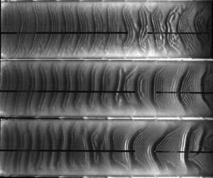
Figure 6 displays shadowgraphs of the film surface and the corresponding spatiotemporal diagrams for different gas velocities at  $\textit {Re}_l=35$ and $f=2.8$ Hz. Increasing the gas velocity generates interactions between waves that can induce coalescence events, clearly visible in figure 6( f), resulting in solitary waves of high amplitude preceded by numerous capillary ripples in the downstream portion of the plane (figure 6c,e). The initial regular wavetrain is progressively disrupted by the counter-current gas flow as one moves downstream, but it remains globally 2-D before merging occurs. In this study, we are interested in this region of 2-D travelling waves, so measurements are performed at the location indicated by the white mark in figures 6(a), 6(c) and 6(e). In particular, we wish to know the nonlinear response of these waves to the strongly confined counter-current gas flow.

Figure 6. (a,c,e) Shadowgraphs of the gas–liquid interface over the entire test section for three different gas velocities, (b,d, f) associated spatiotemporal diagrams. Here (a,b)  $u_g=1.9\ {\rm m}\ {\rm s}^{-1}$ ( $\textit {Re}_g=587$), (c,d) $u_g=3.4\ {\rm m}\ {\rm s}^{-1}$ ( $\textit {Re}_g=1023$), (e, f) $u_g=4.1\ {\rm m}\ {\rm s}^{-1}$ ( $\textit {Re}_g=1242$). These figures are the continuation of the aerostatic case ( $u_g=0$) presented in figure 4. The white dot and arrow are the same as those described in the caption of figure 4. Here $\textit {Re}_l=35$, $f=2.8$ Hz, $\eta _0=11.1$.
3.1. Effect of confined counter-current gas flow on 2-D saturated travelling waves
In this section, we confront the results obtained in our strongly confined channel with previous experiments conducted in a larger channel (Kofman et al. Reference Kofman, Mergui and Ruyer-Quil2017). We consider a liquid film flowing at  $\textit {Re}_l=35$ on which we force travelling waves of frequency $f=2.8$ Hz through our coherent inlet forcing. We are interested in studying the effect of the counter-current gas flow on these waves, and, in particular, how this effect changes depending on the channel height.
Figure 7 confronts time records of the film thickness for the  $H=19$ mm channel (figure 7a–c), which corresponds to a relative confinement $\eta _0=39$ (Kofman et al. Reference Kofman, Mergui and Ruyer-Quil2017), with those measured in our strongly confined $H=5.2$ mm channel (figure 7d–f), where $\eta _0=11.1$. The measurement point was located at $x=60$ cm from the liquid inlet in both experiments. Without imposed gas flow ( $u_g=0$, figure 7a,d) the wave train is identical in both cases, consisting of waves with a large-amplitude asymmetric hump preceded by three capillary ripples. Thus, the level of confinement is inconsequential for the aerostatic configuration. Starting from this reference state, we compare the response of solitary waves with a gradual increase of the gas velocity for both confinements (figure 7b,e,c, f). The striking difference between the two cases is that the maximum film height gradually increases with $u_g$ in the large channel whereas it levels off in the strongly confined case. We also observe that the counter-current air flow attenuates the capillary ripples ahead of the main hump, as discussed in Kofman et al. (Reference Kofman, Mergui and Ruyer-Quil2017). This effect is much more pronounced in the strongly confined channel.

Figure 7. Influence of the gas velocity  $u_g$ on nonlinear wave profiles for two confinement levels: $\eta _0=39$ ( $H=19$ mm) and $\eta _0=11.1$ ( $H=5.2$ mm); $\textit {Re}_l=35$, $f=2.8$ Hz, $x=60$ cm. Here (a) $\eta _0 = 39$, $u_g = 0\ {\rm m}\ {\rm s}^{-1}$; (b) $\eta _0 = 39$, $u_g = 3.3\ {\rm m}\ {\rm s}^{-1}$; (c) $\eta _0 = 39$, $u_g = 4.4\ {\rm m}\ {\rm s}^{-1}$; (d) $\eta _0 = 11.1$, $u_g = 0\ {\rm m}\ {\rm s}^{-1}$; (e) $\eta _0 = 11.1$, $u_g = 3.4\ {\rm m}\ {\rm s}^{-1}$; ( f) $\eta _0 = 11.1$, $u_g = 4.4\ {\rm m}\ {\rm s}^{-1}$.
Figure 8 quantifies the gas effect on the wave characteristics for these two confinement levels. Figure 8(a) displays the effect of the gas on the wave velocity,  $c$, and figure 8(b) its effect on the minimal ( $h_{min}$), averaged ( $h_{m}$) and maximal ( $h_{max}$) values of the film thickness. We find that the slowing of the waves caused by the counter-current flow is more pronounced in the strongly confined channel than in the larger one. Figure 8(b) shows that $h_{min}$ and $h_{max}$ are influenced by the confinement. $h_{min}$ slightly increases with $u_g$ in the strongly confined channel while it remains constant in the large channel, or even slightly decreases for high gas velocities. As shown in figure 7, $h_{max}$ in the strongly confined channel increases with $u_g$ in a first stage ( $u_g < 2.1\ {\rm m}\ {\rm s}^{-1}$ for $\eta _0=11.1$) then saturates, whereas it continuously increases in the large channel. By contrast, $h_m$ increases by the same amount with $u_g$ in all experiments, regardless of the confinement level. In order to account for this increase in the mean film thickness, we report in figure 9 the normalized quantities
 \begin{equation} \delta_{max} = \frac{h_{max}}{h_{m}} \end{equation}
based on the data from figure 8(b).

Figure 8. Influence of the gas velocity  $u_g$ on: (a) wave celerity $c$, (b) minimum $h_{min}$ (downward triangles), mean $h_{m}$ (squares) and maximum $h_{max}$ (circles) film thickness for $\eta _0=39$, $\eta _0 =11.1$ and $\eta _0 =9.9$ (white, grey and black symbols, respectively). Here $\textit {Re}_l=35$, $f=2.8$ Hz, $x=60$ cm. Error bars are drawn for all symbols, but most of them are shorter than the symbol size in panel (b) and thus invisible.

Figure 9. Influence of the gas velocity  $u_g$ on $\delta _{max}$ (3.1) for $\eta _0=39$, $\eta _0 =11.1$ and $\eta _0 =9.9$ (white, grey and black symbols, respectively). Here $\textit {Re}_l=35$, $f=2.8$ Hz, $x=60$ cm.
For  $\eta _0=39$ ( $H=19$ mm), $\delta _{max}$ monotonously increases with $u_g$ (open circles). Thus, increasing the gas flow rate amplifies the nonlinear waves, which implies a destabilizing (nonlinear) effect. This behaviour has been reported in several numerical studies (Trifonov Reference Trifonov2010, Reference Trifonov2019; Tseluiko & Kalliadasis Reference Tseluiko and Kalliadasis2011). By contrast, for the strongly confined channel, $\delta _{max}$ first increases but then clearly decreases with $u_g$ (filled circles), in particular for $\eta _0=9.9$. These results confirm experimentally the numerical finding of Lavalle et al. (Reference Lavalle, Mergui, Grenier and Dietze2021) that increasing the counter-current gas flow can attenuate nonlinear waves.
For the strongly confined channel, the attenuation of nonlinear waves observed in figure 9 sets in at  $u_g > 2\ {\rm m}\ {\rm s}^{-1}$. As shown in figure 8(a), this coincides with a sharp drop in wave celerity under the effect of the gas which is much more pronounced in the strongly confined channel than in the large channel. In figure 9, the wave amplitude curve $\delta _{max}(u_g)$ exhibits a saw-tooth shape during the stabilizing stage ( $u_g > 2\ {\rm m}\ {\rm s}^{-1}$) that will be discussed in the next subsection. For $\eta _0=11.1$ (grey symbols) the increase in $\delta _{max}(u_g)$ which reflects a redestabilization of the waves between $u_g=2.9\ {\rm m}\ {\rm s}^{-1}$ and $u_g=3.3\ {\rm m}\ {\rm s}^{-1}$ is correlated to the modulation in the wave celerity depicted in figure 8(a) (grey symbols) which means that the stabilization mechanism is very sensitive to the wave celerity.
3.2. Effect of the counter-current gas flow on precursory capillary ripples
The saw-tooth shape exhibited in figure 9 for the strongly confined channel at  $u_g > 2.1\ {\rm m}\ {\rm s}^{-1}$ is correlated to the wave celerity and results in a sequential suppression of capillary ripples under the effect of an increasing gas flow, as shown in figure 10, where wave profiles at different gas velocities are displayed for $\eta _0=9.9$ (black symbols in figure 9). For $u_g<2.1\ {\rm m}\ {\rm s}^{-1}$ the effect of the counter-current gas is to increase the wave amplitude without significantly affecting the wave speed and the number of capillary ripples remains unchanged (in this case, three capillary ripples are observed ahead of the main hump). For $u_g>2.1\ {\rm m}\ {\rm s}^{-1}$, the wave speed drops significantly, which reduces the wavelength of the main waves ( $f=2.8$ Hz is constant here). Both effects are known to reduce the number and amplitude of precursory capillary ripples (Dietze Reference Dietze2016), and this is observed in figure 10 ( $\eta _0=9.9$): we move from three to two capillary ripples between $u_g=2.9\ {\rm m}\ {\rm s}^{-1}$ (alternation of two or three capillary ripples) and $u_g=3.1\ {\rm m}\ {\rm s}^{-1}$ (two capillary ripples) and from $2$ to $1$ at $u_g=3.8\ {\rm m}\ {\rm s}^{-1}$ just before flooding. For $\eta _0=11.1$ (grey symbols in figure 9) the transition $3\to 2$ and $2\to 1$ occurs at $u_g \simeq 2.6 {\rm m}\ {\rm s}^{-1}$ and $3.6\ {\rm m}\ {\rm s}^{-1}$. The change in the number of capillary ripples correspond to the troughs of the saw-tooth shape in figure 9.

Figure 10. Influence of the gas velocity  $u_g$ on nonlinear wave profiles measured at $x=60$ cm for $\textit {Re}_l=35$, $f=2.8$ Hz, $\eta _0=9.9$, corresponding to the experiment presented in figure 9 (black symbols). Here (a) $u_g = 0\ {\rm m}\ {\rm s}^{-1}$; (b) $u_g = 0.8\ {\rm m}\ {\rm s}^{-1}$; (c) $u_g = 1.6 {\rm m}\ {\rm s}^{-1}$; (d) $u_g = 2.1\ {\rm m}\ {\rm s}^{-1}$; (e) $u_g = 2.4\ {\rm m}\ {\rm s}^{-1}$; ( f) $u_g = 2.7\ {\rm m}\ {\rm s}^{-1}$; (g) $u_g = 2.9\ {\rm m}\ {\rm s}^{-1}$; (h) $u_g = 3.1\ {\rm m}\ {\rm s}^{-1}$; (i) $u_g = 3.4\ {\rm m}\ {\rm s}^{-1}$; (j) $u_g = 3.7\ {\rm m}\ {\rm s}^{-1}$; (k) $u_g = 3.8\ {\rm m}\ {\rm s}^{-1}$; (l) $u_g = 4\ {\rm m}\ {\rm s}^{-1}$.
To confirm that the number of capillary ripples is indeed governed by the wave speed, figure 11 compares the maximum positive slope,  $\mathrm {max}\{\partial _xh\}$, for the two confinement levels $\eta _0=11.1$ (grey symbols) and $\eta _0=39$ (white symbols). This maximum is observed at the back of the first capillary ripple (squares in figure 3b) and is an indicator of the compression of the capillary wave train due to the decrease of the wavelength. Figure 11(a) displays $\mathrm {max}\{\partial _xh\}$ (square symbols) as a function of $u_g$, and figure 11(b) as a function of the normalized wave velocity $\hat {c}$, i.e.
 \begin{equation} \hat{c}=\frac{c_0 - c}{c_N}, \end{equation}
where  $c_N= {g h_N^2 \sin \beta }/{\nu _l}$ is the speed of kinematic waves in a passive atmosphere, $c_0$ corresponds to the measured wave speed in the case of a quiescent gas, and $h_N=({3\,q_l\,\nu _l}/{\sin \beta g})^{1/3}$ is the Nusselt thickness (the flat-surface film thickness in the passive-gas limit).

Figure 11. Influence of the gas velocity  $u_g$ in (a) and the normalized gas velocity $\hat {c}$ (3.2) in (b), on the maximum positive free-surface slope $\mathrm {max}\{\partial _xh\}$ at the back of the first capillary ripple (squares) and at the main hump tail (downward triangles), and on the maximum negative slope $\mathrm {min}\{\partial _xh\}$ at the front of the main hump (upward triangles), for $\eta _0=39$ (white symbols) and $\eta _0 =11.1$ (grey symbols). The number of capillary ripples is indicated. Vertical dashed lines in (b) indicate the values of $\hat c$ related to the wave profiles presented in figure 12. Here $f=2.8$ Hz, $\textit {Re}_l=35$, $x=60$ cm.

Figure 12. Influence of the confinement on wave profiles at given values of  $\hat {c}$ (3.2) marked by vertical dashed lines in figure 11(b). Here (a) $\hat {c}=0.13$; (b) $\hat {c}=0.23$. Thin solid line, $\eta _0=39$ ( $u_g=4.4\ {\rm m}\ {\rm s}^{-1}$ in (a) and $5.5\ {\rm m}\ {\rm s}^{-1}$ in (b)); thick solid line, $\eta _0=11.1$ ( $u_g=2.8\ {\rm m}\ {\rm s}^{-1}$ in (a) and $4\ {\rm m}\ {\rm s}^{-1}$ in (b)). Same parameters as in figure 11.
Figure 11(a) shows that for a given value of  $u_g \neq 0$, the slope magnitude at the back of the first capillary ripple as well as the number of capillary ripples depend on the confinement. By contrast, figure 11(b) shows that for a given value of $\hat {c}$ these quantities are identical regardless of the confinement, which is also clearly visible from wave profiles presented in figure 12 for $\hat {c}=0.13$ and $\hat {c}=0.23$ (marked by vertical dashed lines in figure 11b). This behaviour implies that the capillary region is not directly affected by the gas shear-stress but is controlled by the indirect effect of the gas-induced slowing of the large waves. In figure 11 we have also plotted the maximum negative slope $\mathrm {min}\{\partial _xh\}$ at the main hump front (upward triangles) which is an indicator of the steepness of the wave, and the maximum (positive) slope at the wave tail (downward triangles). In the large channel (white symbols) the front inclination remains unchanged as the gas velocity is increased, while the tail steepens, thus resulting in a more symmetrical wave (thin solid curves in figure 12). By contrast in the strongly confined channel (grey symbols), the front inclination weakens while the tail slope remains unchanged under the action of the counter-current flow, and the resulting wave is less symmetric than in the large channel (thick solid curves in figure 12).
3.3. Influence of the liquid Reynolds number
We now investigate the effect of the counter-current gas flow on the response of nonlinear waves for different values of the liquid Reynolds number  $\textit {Re}_l$ and the forcing frequency $f$, in the strongly confined channel. As shown in figure 13 for the quiescent-gas reference case, these parameters clearly affect the mean film thickness and consequently the confinement level $\eta _0$ (2.2), the maximum film thickness $h_{max}$ and the number of precursory capillary ripples. The forcing frequency has been empirically adjusted from the aerostatic case according to the liquid Reynolds number, in order to generate 2-D saturated quasi-solitary waves in the working zone. The resulting wavelength of the unsheared wave train is specified in the caption of figure 13 provided that wave velocity measurements are available.

Figure 13. Wave profiles for different values of the liquid Reynolds number  $\textit {Re}_l$ and forcing frequency $f$ in the strongly confined channel for the aerostatic case. From left to right, the resulting wavelength is $6.5$ cm ( $\textit {Re}_l=22$), $6.5$ cm ( $\textit {Re}_l=35$), $7.3$ cm ( $\textit {Re}_l=44.6$), not available for $\textit {Re}_l=49$. Here (a) $R_l = 22$, $f = 2.2\ {\rm Hz}$, (b) $R_l = 35$, $f = 2.8\ {\rm Hz}$, (c) $R_l = 44.6$, $f = 2.8\ {\rm Hz}$, (d) $R_l = 49$, $f = 3.05\ {\rm Hz}$.
We report in figure 14 the variation of  $c$ (figure 14a) and $\delta _{max}$ (figure 14b) in terms of $\textit {Re}_g$ for different $\textit {Re}_l$ and forcing frequency $f$. For $\textit {Re}_l=44.6$ (grey triangles), we observe the same overall behaviour as for $\textit {Re}_l=35$, which was presented in the previous section. In a first stage, $\delta _{max}$ increases with $\textit {Re}_g$ (the gas flow is nonlinearly destabilizing) then decreases when $c$ is significantly reduced (the gas flow is nonlinearly stabilizing), with saw-tooth modulations associated with the change in the number of capillary ripples, whereas the variation of $c$ with $\textit {Re}_g$ remains monotonous. For a higher liquid flow rate, $\textit {Re}_l=49$ (crosses), the destabilizing stage at low gas velocity is replaced by a stabilizing one. For the lowest Reynolds number, $\textit {Re}_l=22$ (open triangles), there are only two capillary waves to start with (figure 13a) and we observe a weak stabilization until $\textit {Re}_g\approx 600$, associated with the suppression of one capillary wave. Then $\delta _{max}$ increases to reach a constant value while maintaining one capillary wave until the experiment breaks down due to flooding downstream.

Figure 14. Influence of the liquid Reynolds number  $\textit {Re}_l$ on: (a) wave celerity, $\textit {Re}_l=22$, $\eta _0=11.5$ (white triangles) – $\textit {Re}_l=35$, $\eta _0=11.1$ (black triangles) – $\textit {Re}_l=44.6$, $\eta _0=10.3$ (grey triangles); (b) $\delta _{max}=h_{max}/h_{m}$, same parameters as (a) for white and grey triangles, $\textit {Re}_l=35$, $\eta _0=9.9$ (black circles) – $\textit {Re}_l=49$, $\eta _0=10.3$ (crosses). strongly confined channel.
We now introduce the local relative confinement parameter  $\eta _{max}$ as
 \begin{equation} \eta_{max}=\frac{H}{h_{max}}. \end{equation}
 Figure 15 displays  $\eta _{max}$ as a function of $\textit {Re}_g$ for the same parameters as figure 14. The gas-induced stabilization at $\textit {Re}_l=22$ is associated with a relative confinement $\eta _{max} \approx 9$. For $\textit {Re}_l=35$, $45$ and $49$ the stabilizing effect occurs for smaller confinement levels.


3.4. Effect of the surface waves on the mean film thickness
We now wish to gauge the effect of the gas-sheared surface waves on the mean film thickness  $h_m$. In particular, we wish to know whether $h_m$ is decreased or increased versus the primary-flow thickness. In the case of a passive gas or a quiescent unconfined atmosphere, it is well known that $h_m$ is smaller than the primary-flow thickness. This is known as wave-induced effective film thinning (Miyara Reference Miyara1999). In our current case of a counter-current gas flow, it turns out that the wave effect depends on the confinement level. To group our measurement data for the $H=5$ mm channel, where the gas flow is laminar, and the data of Kofman et al. (Reference Kofman, Mergui and Ruyer-Quil2017) for an $H=19$ mm channel, where the gas flow is turbulent, we introduce the Froude number $Fr_{g,l}$, which relates interfacial shear stress ( ${\sim }\rho _g u_{g}^2$) to gravitational effects,
 \begin{equation} Fr_{g,l}=\sqrt{\frac{\rho_g u_{g}^2}{\rho_l g \sin \beta h_N}}, \end{equation}
and the normalized film thickness  $\hat {h}$, i.e.
 \begin{equation} \hat{h}=\frac{h_m}{h_{m}^0}-1. \end{equation}
 Figure 16(a) displays  $\hat {h}$ as a function of $Fr_{g,l}$, for all experiments conducted in the $H=5$ mm channel (different $\textit {Re}_l$ and $f$), as well as the experiments of Kofman et al. (Reference Kofman, Mergui and Ruyer-Quil2017) conducted in a $H=19$ mm channel (square symbols). The experimental data collapse onto two different trends, one for the narrow channel and another for the wide channel. This is due to the different flow regimes in the two configurations, the gas flow being laminar in the former case and turbulent in the latter.

Figure 16. Relative mean film thickness  $\hat {h}$ (3.5) measured in the $H \approx 5$ mm channel and in the $H \approx 19$ mm channel (Kofman et al. Reference Kofman, Mergui and Ruyer-Quil2017, square symbols), as a function of: (a) the Froude number $Fr_{g,l}$ (3.4); (b) the modified Froude number, $Fr_{fric}$ (3.6). The solid (laminar gas flow) and dashed (turbulent gas flow) curves correspond to the flat-film solution $\hat {h}_{flat}$ according to (B13) with $\epsilon =0$ ( $\hat {h}_{flat}=\tilde {h}_{flat}-1$).
To account for this, we improve our approximation of the interfacial shear stress used in (3.4) in a modified gas–liquid Froude number,  $Fr_{fric}$, based on the friction velocity, $u_{fric}$, as follows:
 \begin{equation} Fr_{fric}=\sqrt{\frac{\rho_g u_{fric}^2}{\rho_l g \sin \beta h_N}}=\sqrt{\frac{C_{f,i}}{2}} Fr_{g,l}, \end{equation}
where  $u_{fric}$ is based on the tangential interfacial gas shear stress of the primary flow (no waves), $\tau _i$, as
 \begin{equation} u_{fric}=\sqrt{\frac{\tau_i}{\rho_g}}. \end{equation}
 Here  $\tau _i$ is related to the global skin-friction coefficient, $C_{f,i}$, as follows:
 \begin{equation} C_{f,i}=\frac{\tau_i}{1/2 \rho_g u_g^2}. \end{equation}
 In the strongly confined channel, the gas flow is laminar and we approximate  $C_{f,i}$ by the relation for Poiseuille flow through a plane dry channel,
 \begin{equation} C_{f,i}=12 \textit{Re}_g^{{-}1}. \end{equation}
In the large channel the gas flow is fully turbulent and we use an experimental correlation established by Patel & Head (Reference Patel and Head1969) in a wide rectangular horizontal dry channel,
 \begin{equation} C_{f,i}=0.0376 \textit{Re}_{g}^{{-}1/6}. \end{equation}
 Using these correlations for  $C_{f,i}$, we assume that the liquid–gas interface can be considered as immobile. To validate this motionless interface assumption, we have compared the film thickness of a flat-surface film subject with a counter-current laminar gas flow as obtained by numerical solution of the fully coupled two-phase primary flow (Lavalle et al. Reference Lavalle, Li, Mergui, Grenier and Dietze2019) with the thickness obtained by assuming an interphase skin friction coefficient according to (3.9). Details on this flat-film model are given in Appendix B. The two predictions are in excellent agreement and this holds over the entire range of experimental conditions studied in this work (see figure 23 in Appendix B).
In figure 16(b),  $\hat {h}$ (3.5) is plotted as a function of $Fr_{fric}$, according to (3.6). We observe that the new scaling is more appropriate to describe the effect of the shear stress exerted by the gas on the interface, as the laminar and turbulent data are now gathered. The two additional solid and dashed curves correspond to the flat-film model $\hat {h}_{flat}$ (according to (B13) with $\epsilon =0$, $\hat {h}_{flat}=\tilde {h}_{flat}-1$) for the laminar gas flow in the strongly confined channel (solid line) and for the turbulent gas flow in the large channel (dashed line). This model represents a reference solution for comparison with the wavy experimental data.
The mean film thickness results from two opposing intricate effects: the well-known effective thinning due to nonlinear surface waves, illustrated in figure 5 for the aerostatic case; and the thickening effect of the counter-current gas flow produced by the interfacial shear-stress. The relative competition of these two effects determines the mean film thickness ultimate behaviour.
In the large channel (square symbols) the experimental data lie slightly below the flat-film prediction. Thus, surface waves tend to reduce the mean film thickness, as in the case of a quiescent atmosphere.
In the strongly confined channel, at high liquid Reynolds number values  $\textit {Re}_l$ and high Froude numbers ( $Fr_{fric} \geqslant 0.35$), experimental data are clearly above the flat-film prediction which means that the mean wavy film thickness grows faster than the reference flat-film thickness. This behaviour occurs in the nonlinear stabilizing regime for strong relative confinement levels, where surface waves promote a significant variation of the gas cross-section, which in turn affects the local tangential shear stress. This is the basis for the linear stabilization mechanism described by Lavalle et al. (Reference Lavalle, Li, Mergui, Grenier and Dietze2019). In this regime, the gas effect tends to reduce the nonlinear amplitude of the main hump and thus the thinning effect of the waves, while it increases the residual flat film thickness between two humps. In figure 14(b), we observe that during this stage, the interaction between the liquid film and the counter-current gas flow generates strong disturbances of the wave train as highlighted by the large temporal fluctuations measurements for $\textit {Re}_l=44.6$ and $49$.
$49$.
By contrast, when  $\textit {Re}_l$ and thus the wave amplitude is small, experimental data are well predicted by the flat-film model over the entire range of the Froude number. In this case, the mean thickness of the wavy film increases at the same rate as the flat film thickness when the gas flow rate is increased, indicating that the thinning effect of the surface waves balances the overall thickening effect due to the gas shear stress. This balance can also be observed at higher $\textit {Re}_l$ and moderate Froude number values ( $Fr_{fric} \leqslant 0.35$, crosses) for experiments concerned with the monotonously nonlinear stabilizing regime (see crosses in figure 14b).
Further, we conclude that the interfacial shear stress effect on the nonlinear surface waves changes by increasing the gas velocity in the strongly confined channel. This behaviour could be related to the observations of Trifonov (Reference Trifonov2019), who performed simulations of nonlinear waves for a set of parameters similar to our experimental conditions ( $\beta =5^{\circ }$, $H=5$ mm, $\textit {Re}_l=5$, $15$ and $40$, see the supplementary material associated with the cited article). The author demonstrates the existence of a local minimum of the mean film thickness and of the gas friction coefficient in terms of the gas superficial velocity. More specifically, at $\textit {Re}_l=40$, he found that the decrease of the friction coefficient deviates from the decreasing trend of the waveless solution ( $\propto 1/ \textit {Re}_g$) at a gas velocity comparable to the experimental values associated with the deviation of $h_m$ from the flat-film solution observed in figure 16(b).
The experimental data corresponding to the black filled circles deviates from the other data at similar liquid Reynolds numbers. For this experiment the Kapitza number is lower (by 13 % due to a different ambient temperature) and the channel height  $H$ is slightly lower (by $4\,\%$). These variations do not significantly affect the primary flow, as can be inferred from the right-hand-pointing triangles which correspond to an experiment performed the same day without inlet forcing, and which lie on the solid curve related to the primary flow solution. However, the destabilizing effect of the gas on the nonlinear waves at moderate Froude number values may be enhanced, which could favour the wave-induced effective film thinning effect (these data lie below the solid curve).
4. Conclusion
In this paper, experiments were conducted on water films falling along the bottom wall of a weakly inclined ( $\beta =4.9^{\circ }$) rectangular channel of height $H \approx 5$ mm interacting with a laminar counter-current air flow. Surface waves were excited via coherent inlet forcing before they come into contact with the air flow to promote travelling waves consisting of a large-amplitude hump preceded by capillary ripples. We focused on the sheared region of the film where the waves were 2-D without interaction between them. Local film thickness time traces and wave celerity measurements have been performed together with visual observations.
The effect of the air flow on the height, shape and speed of the waves was investigated and contrasted with results obtained by Kofman et al. (Reference Kofman, Mergui and Ruyer-Quil2017) in a channel of height  $19$ mm, where the counter-current gas flow was turbulent. The stronger confinement level studied here versus the experiments of Kofman et al. (Reference Kofman, Mergui and Ruyer-Quil2017) not only changes the geometrical constriction of the gas flow but also leads to a laminar flow regime in the gas instead of a turbulent one. In experiments, these two effects, which play their own distinct roles, cannot be decoupled. However, Trifonov (Reference Trifonov2010) has shown via numerical simulations that the main effect of turbulence is to shift the onset of wave-induced critical events (e.g. the flooding onset) towards lower superficial gas velocities.
In our experiments, no confinement-induced effect was detected on the wave dynamics in the case of a quiescent gas. Indeed, the shape, amplitude and velocity of the nonlinear waves excited at a prescribed frequency are almost identical for the two confinement levels. When a counter-current gas flow is imposed, striking differences are observed. For all the experiments conducted in the weakly confined channel, the effect of the gas on the travelling nonlinear waves was destabilizing (see Kofman et al. Reference Kofman, Mergui and Ruyer-Quil2017), whereas a monotonic stabilizing effect or a non-monotonic trend was observed in the strongly confined channel, depending on the liquid Reynolds number  $\textit {Re}_l$.
For small  $\textit {Re}_l$ in the strongly confined channel, inertia is weak and the relative confinement is quite low without gas flow ( $\eta _{max}>9$). Under these conditions, the wave amplitude first slightly diminishes as the gas velocity is increased and then increases to reach a plateau sustaining one capillary ripple until onset of flooding. In that case, the stabilizing mechanism induced by the variation of the gas shear stress at the interface is quite weak.
For moderate  $\textit {Re}_l$, the wave amplitude first increases with the gas velocity while the number of capillary ripples ahead of the main hump and the wave celerity remain unchanged. Upon increasing the gas velocity further, the wave amplitude diminishes and a gradual reduction of the number of capillary ripples is observed. For higher values of $\textit {Re}_l$, a monotonically gas-induced wave attenuation is observed.
These experimental observations are in line with recent numerical results obtained by Lavalle et al. (Reference Lavalle, Mergui, Grenier and Dietze2021) in a superconfined channel, where monotonic gas-induced amplification (attenuation) of the nonlinear wave amplitude was detected for larger (smaller)  $H$, and a non-monotonic trend was observed for intermediate $H$.
$H$.
To quantify the effect of surface waves on the mean film thickness in a universal form, a modified Froude number has been constructed which relates viscous drag based on the skin friction coefficient and gravity. We have compared the normalized measured mean film thickness  $\hat {h}$ with the primary-flow solution $\hat {h}_{flat}$ obtained in the limit of a frozen (immobile) liquid–gas interface. In the case of a turbulent gas flow, which corresponds to experiments conducted in the large channel, $\hat {h}_{flat}$ is greater than $\hat {h}$. In these experiments, waves are significantly amplified by the counter-current flow and the wave-induced film thinning effect (Miyara Reference Miyara1999) is dominant compared with the thickening effect of the gas shear stress. In the laminar configuration, which corresponds to experiments conducted in the strongly confined channel, $\hat {h}$ and $\hat {h}_{flat}$ correspond when $\textit {Re}_l$ is small, which implies that the thinning effect of the waves on the mean thickness is balanced by the shear-stress thickening effect, and the experimental behaviour is well predicted by the model. For higher liquid Reynolds number values, $\hat {h}_{flat}<\hat {h}$ in the range of parameters where the nonlinear stabilization occurs.
Large-scale three-dimensional flow structures may arise in the gas flow and generate a non-zero spanwise tangential Reynolds/viscous stress at the liquid–gas interface. This stress may produce/enhance a spanwise variation of the film height and thus have a direct effect on the mean height  $\hat {h}$ plotted in figure 16(b). Such an effect is not accounted for in $Fr_{fric}$ (3.6), which is based on the streamwise tangential stress at the liquid–gas interface. In our current strongly confined experiments, where the gas flow is laminar, we can exclude a three-dimensional effect, as the wavefronts shown in figure 6 are quasi-2-D across the measurement range. In the weakly confined case of Kofman et al. (Reference Kofman, Mergui and Ruyer-Quil2017), where the gas flow is turbulent, wavefronts do display spanwise variations beyond a certain gas velocity (see figure 3 in that paper). Nonetheless, the corresponding data points in figure 16(b) are closely grouped. This either means that the effect of the spanwise component of the interfacial tangential gas shear stress on the film height is much weaker than that of the streamwise component for the studied conditions, or that the two effects are correlated.
Funding
This work was supported by the ANR WavyFilm project, grant ANR-15-CE06-0016-01 of the French Agence Nationale de la Recherche. The authors are grateful to J. Amrani, A. Aubertin, L. Auffray and R. Pidoux for their contribution to build the experimental set-up.
Declaration of interests
The authors report no conflict of interest.
Appendix A. Measurement of the gas flow rate
In this section we describe the procedure that has been used to quantify the air flow rate  $q_g$ generated by the fan in the inclined strongly confined channel of figure 1. This quantity is used to evaluate the gas Reynolds number according to (2.3). This was done based on a calibration curve between a given fan power and the corresponding gas flow rate obtained from velocity measurements in the dry channel, i.e. without the liquid film. The porous medium at the end of the bottom glass plate was replaced by a Plexiglas plate with an opening to allow access for a hot-wire anemometer probe (see figure 17). With this probe, we measured the wall-normal profile of the streamwise velocity $u(y)$ at the midwidth of the channel and $4.5$ cm from the air inlet. Figure 18 displays profiles obtained for different fan powers and for the inclination angle used in the experiments, $\beta =4.9^{\circ }$. Each dot corresponds to a time-averaged measurement over $30$ s and the error bars are included according to the uncertainty of the probe given by the manufacturer. A polynomial fit is performed for each profile from which we compute the air flow rate,
 \begin{equation} q_g=W \int_{0}^{H} u(y) \, \mathrm{d} y, \end{equation}
where  $W=27$ cm is the channel width. The calibration curve presented in figure 19 gives the air flow rate per unit width as a function of the imposed fan power, $P_f$. The gas Reynolds number, $\textit {Re}_g$, is then calculated using (2.3). When the fan is switched off ( $P_f=0$), there is no gas flow in the dry channel, and, thus, $\textit {Re}_g=0$ according to our procedure, even though a small non-zero gas flow would be generated in the presence of a falling liquid film.

Figure 17. Location of the anemometer used to measure the air velocity at the end of the channel (gas inlet).

Figure 18. Air velocity profiles measured for different fan powers (in Watts) in the dry channel:  $P_f=1.3$ (circles); $3.9$ (squares); $6.5$ (upward triangles); $7.8$ (downward triangles); $10.4$ (open circles); and $13$ (open squares). Solid lines correspond to polynomial fits. Here $\beta =4.9^{\circ }$.

Figure 19. Calibration curve used to quantify the gas flow rate  $q_g$ (A1) per unit of channel width from the imposed fan power $P_f$. Here $\beta =4.9^{\circ }$.
In figure 18, we have plotted several examples of measured velocity profiles for laminar flow conditions (black symbols), i.e.  $\textit {Re}_g<1300$ according to the laminar–turbulent transition threshold determined by Patel & Head (Reference Patel and Head1969) in a high-aspect-ratio channel. Table 1 reports the corresponding values of the velocity ratio $u_g/u_{max}$, where the mean velocity $u_g$ has been defined in (2.4) and $u_{max}$ is the maximum velocity. The aerodynamic entry length, $L_d$, is also reported, which is defined as the length needed for the boundary layers along the two horizontal channel walls to join at $y=H/2$. Based on the presumption that air enters the channel with a uniform velocity profile and using the Blasius correlation, it is straightforward to show that
 \begin{equation} \frac{L_d}{H}=0.01 \textit{Re}_g. \end{equation}
Table 1. Ratio between the mean and the maximum air velocity issued from the measured velocity profiles (black symbols in figure 18) and the corresponding aerodynamic entry lengths given by (A2).

Based on this data, it is clear that the gas flow is fully developed in the entire region of the channel used for our falling liquid film experiments.
A specific velocity measurement series has been performed to confirm the laminar–turbulent transition threshold determined by Patel & Head (Reference Patel and Head1969). The top glass plate of the channel was replaced by a Plexiglas plate with an opening to allow access for the probe far from the air entrance (approximately  $1$ m away). In this campaign, only the maximum air velocity, $u_{max}$, has been measured for different fan powers. By assuming that the flow is laminar and fully developed at this location, i.e. $u_g \approx 0.667 u_{max}$, we can calculate a flow rate and then a Reynolds number, $\textit {Re}_{g}^{lam}$. For a given fan power, we compare $\textit {Re}_{g}^{lam}$ with $\textit {Re}_g$ issued from the complete vertical velocity profiles (using (A1) then (2.3)). Figure 20 displays $\textit {Re}_g^{lam}$ and $\textit {Re}_{g}$ against the imposed fan power. It can be seen that for $\textit {Re}_g \leqslant 1200$ the points collapse, which means that $\textit {Re}_g=\textit {Re}_{g}^{lam}$ and thus the flow is confirmed to be laminar. The discrepancy observed for $\textit {Re}_g > 1200$ means that the flow is no longer laminar. From these measurements we can conclude that in our inclined channel, the laminar–turbulent transition occurs for $\textit {Re}_g$ slightly greater than $1200$.

Figure 20. Here  $\textit {Re}_g$ (filled circles) and $\textit {Re}_{g}^{lam}$ (open circles) as a function of the fan power $P_f$. Here $\textit {Re}_g$ is calculated by integrating velocity profiles measured at the end of the channel (figure 18), and $\textit {Re}_{g}^{lam}$ from the maximum velocity measurements performed in the fully developed region and assuming a laminar parabolic profile, i.e. $u_g = 2/3 u_{max}$.
The gas Reynolds number,  $\textit {Re}_g$, defined in (2.3) can be used to characterize the counter-current air flow in the experiments provided that the gas flow rate circulating into the experimental gas loop is not affected by the presence of the liquid film in the channel at a fixed fan power. The validity of this assumption is discussed below.
For a gas flowing in a dry rectangular channel with a large transversal aspect ratio of length  $L$ and height $H$ (in our configuration $W/H=54 \gg 1$), the pressure drop is given by the analytic relation $\Delta p_{channel} = 4 C_f ({L}/{2 H})\frac {1}{2} \rho _g ({q}/{H})^2$ where $q=u_g H$ is the volumetric gas flow rate (per unit width, i.e. $q=q_g/W$) and $C_f$ is the skin friction coefficient, with $C_f=12/Re_g$. Thus, $\Delta p_{channel} \propto q/H^3$ and the corresponding power $P_{channel} = q \Delta p_{channel} \propto q^2/H^3$. For a given power value $P_{channel}$, decreasing the channel height by $10\,\%$ (typical to the reduction due to the presence of the liquid film in the experiments) leads to a $15\,\%$ decrease in the flow rate. However, $\Delta p_{channel}$ constitutes only a small part of the total pressure drop, which is dominated by the resistance in the section between the outlet slot and the fan. Thus, the actual decrease in $q_g$ upon decreasing $H$ by 10 % is relatively low. For the range of parameters considered in this study, we have estimated it to be less than $5\,\%$.
Appendix B. Flat-film model for laminar and turbulent gas flow
In figure 16(b), we have estimated the liquid film thickness of the flat-surface primary flow based on the skin friction coefficient  $C_{f,i}$. This approach allows us to account for a laminar or turbulent gas flow within the flat-film model. For laminar flow, this coefficient $C_{f,i}$ is given by (3.9) and for turbulent flow by (3.10), according to the experiments of Patel & Head (Reference Patel and Head1969). However, these experiments were performed in a dry channel, and, thus, our flat-film model implies an immobile liquid–gas interface. The current appendix aims to verify this assumption. We do this based on the laminar case, which is the limiting one, and for which we can easily obtain a reference solution for the flat-surface film based on the fully coupled primary flow (Lavalle et al. Reference Lavalle, Li, Mergui, Grenier and Dietze2019).
The gas velocity profile for the fully coupled primary flow is given by
 \begin{equation} u(Y) = \frac{-K_g}{2 \mu_g} H_g^2 \left(Y-Y^2\right)+u_0 \left(1-Y\right), \end{equation}
where  $K_g$ reads
 \begin{equation} K_g = \left({\partial_x p}- \rho_g g \sin\beta \right), \end{equation}
where  $\partial _x p$ is the driving longitudinal pressure gradient, positive in our case for a counter-current gas flow, and $Y=(y-h_{flat})/H_g$, with $h_{flat}$ denoting the flat-surface film thickness and $H_g = H -h_{flat}$ the height of the gas cross-section. Here $u_0$ is the liquid velocity at the film surface ( $u_0>0$).
The gas velocity averaged over  $H_g$ can be written as
 \begin{equation} u_{g}^+ = \frac{-K_g}{12 \mu_g} H_g^2 + \frac{u_0}{2} = u_{g}^{0} + \frac{u_0}{2} = u_{g}^{0} \left(1+\frac{\epsilon}{2} \right), \end{equation}
where  $u_{g}^{0}$ corresponds to the average gas velocity in the limit $u_0=0$ and $\epsilon = u_0/u_{g}^{0}$.
The gas Reynolds number is defined as
 \begin{equation} \textit{Re}_{g}^+ = \frac{u_{g}^+ H_g}{\nu_g} = \frac{u_{g}^0 H_g}{\nu_g} + \frac{u_0 H_g}{2 \nu_g} = \textit{Re}_{g}^0 + \textit{Re}_0= \textit{Re}_{g}^0 \left(1+\frac{\epsilon}{2}\right). \end{equation}
 We can write the tangential shear-stress at the liquid–gas interface and at the top wall,  $\tau _{i}$ and $\tau _{w}$, as
 $$\begin{gather} \tau_{i} ={-}\frac{\mu_g}{H_g} \partial_Y u\vert_{Y=0}=\frac{K_g}{2} H_g+ \mu_g \frac{u_0}{H_g } = \tau_{i}^{0} \left(1-\frac{\epsilon}{6}\right), \end{gather}$$
 $$\begin{gather}\tau_{w} = \frac{\mu_g}{H_g} \partial_Y u\vert_{Y=1}= \frac{K_g}{2} H_g - \mu_g \frac{u_0}{H_g} = \tau_{i}^{0} \left(1+\frac{\epsilon}{6}\right), \end{gather}$$
where  $\tau _{i}^{0}= H_g K_g/2$ is the limit of $\tau _i$ and $\tau _w$ for a static interface (i.e. for $\epsilon =0$).
We define the global skin-friction coefficient at the liquid–gas interface,  $C_{f,i}$ as
 \begin{align} C_{f,i} & = \frac{\tau_{i}}{1/2 \rho_g u_{g}^{+^2}} \nonumber\\ & = \frac{\tau_{i}^{0}}{1/2 \rho_g u_{g}^{0^2}} \frac{1-\epsilon /6}{(1+\epsilon /2)^2} = C_{f,i}^0 \frac{1-\epsilon /6}{(1+\epsilon /2)^2}. \end{align}
 In a similar way we can define  $C_{f,w}$ at the top wall as
 \begin{equation} C_{f,w} = C_{f,i}^0 \frac{1+\epsilon /6}{(1+\epsilon /2)^2}, \end{equation}
where  $C_{f,i}^0$ is the skin friction coefficient in the case of static boundaries (i.e. for $\epsilon =0$). In the case of a laminar gas flow, it is given by
 \begin{equation} C_{f,i}^0 = \frac{-12}{\textit{Re}_g^0}. \end{equation}
For convenience, in the experiments  $u_g$ is always taken as positive, therefore $u_g=-u_{g}^{0}$ and $\textit {Re}_g=-\textit {Re}_g^0$ in our counter-current case.
Now, we compute  $C_{f,i}$ and $C_{f,w}$ based on (B7) and (B8), using the liquid velocity at the interface $u_0$ (which enters $\epsilon$) from the fully coupled primary-flow solution. Figure 21(a) displays $C_{f,i}$ (red lines), $C_{f,w}$ (blue lines) and $C_{f,i}^0$ (black line) as a function of the gas Reynolds number $\textit {Re}_g=-\textit {Re}_g^0$ over the range $25<\textit {Re}_g<1500$, for two liquid Reynolds numbers considered in our experiments with $H=5.2$ mm: $\textit {Re}_l=22$ (dashed lines) and $\textit {Re}_l=44.6$ (solid lines). The associated variation of $u_0/u_g = - \epsilon$ is presented in figure 21(b). To specify the range of parameters where the static interface approximation based on the skin-friction coefficient criteria can be considered as valid, we focus on the gas Reynolds values such as the difference between $C_{f,i}$ and $C_{f,i}^0$ is less than $10\,\%$. From figure 21(a) we can conclude that this criterion is met for $\textit {Re}_g>250$ ( $\textit {Re}_l=22$) and $\textit {Re}_g>400$ ( $\textit {Re}_l=44.6$), which corresponds to $u_0/u_g \leqslant 0.08$ in figure 21(b). Figure 21(a) also shows that $C_{f,i} \approx C_{f,w}$ over a range of $u_0/u_g$ where the static interface assumption is no longer valid. For example, the discrepancy between $C_{f,i}$ and $C_{f,w}$ is around $10\,\%$ in figure 21(a) for $(Re_l,Re_g)=(22,80)$ and $(44.6,125)$, corresponding to $u_0/u_g \approx 0.3$ in figure 21(b). This behaviour can be explained by the change in the gas velocity distribution with the gas flow rate. Indeed, the location of the maximum gas velocity is shifted towards the top wall when $u_0/u_g$ is increased by decreasing $\textit {Re}_g$, as shown in figure 22. Consequently, the tangential shear stress is reduced at the liquid–gas interface while it increases at the top wall and the dissymmetry arising from the moving interface is partially attenuated.

Figure 21. (a) Global skin-friction coefficients at the liquid–gas interface  $C_{f,i}$ (B7) (red line) and at the upper wall of the channel $C_{f,w}$ (B8) (blue line) as a function of $\textit {Re}_g$, calculated from the fully coupled primary flow solution. The black line corresponds to a skin-friction coefficient in the case of a static interface (i.e. $\epsilon =0$). (b) Ratio between the interface velocity and the gas velocity $u_0/u_g = -\epsilon$. $\textit {Re}_l=22$ (dashed lines) and $\textit {Re}_l=44.6$ (solid lines), $\beta =4.9^{\,\circ }$, $H=5.2$ mm.

Figure 22. Gas velocity profiles calculated from the fully coupled primary flow solution for  $\textit {Re}_l=22$: $u(Y)/u_{max}$ with $u(Y)$ according to (B1) and $u_{max}=\min (u(Y))<0$. Dash–dot line, $u_0/u_g=1$ ( $\textit {Re}_g=24.3$); dashed line, $u_0/u_g=0.3$ ( $\textit {Re}_g=80$); solid line, $u_0/u_g=0.16$ ( $\textit {Re}_g=145$); thick solid line, $u_0=0$ (Poiseuille flow). The location of $u_{max}$ in the channel, $Y_{max}=Y(u_{max})$, is plotted in the inset as a function of $\textit {Re}_g$ ( $Y_{max}=0.5$ for a Poiseuille flow). Open circles mark $Y_{max}$ for the profiles represented in the figure (except the Poiseuille flow). Here $\beta =4.9^{\circ }$, $H=5.2$ mm.
To go further in testing the validity of this frozen-interface approximation, we will compare the film thickness obtained from the fully coupled primary flow solution with the thickness obtained by assuming an interphase skin friction coefficient according to (B9) using a simple model described below.
We start by writing the velocity profile in the liquid film as
 \begin{equation} u_{l}(y) = \frac{K_l}{\mu_l} \left(h_{flat} y -\frac{y^2}{2}\right)-\frac{\tau_i}{\mu_l}y. \end{equation}
 Here  $K_l$ reads as
 \begin{equation} K_l = \left( (\rho_l-\rho_g) g \sin\beta - \frac{\tau_i+\tau_w}{H-h_{flat}}\right), \end{equation}
where  $\tau _i$ and $\tau _w$ are given by (B5) and (B6), respectively. Therefore, $\tau _i+\tau _w=2 \tau _i^0 = \rho _g u_{g}^{0^2} C_{f,i}^0 = \rho _g u_{g}^2 C_{f,i}^0$.
Integrating (B10) across the liquid layer gives the liquid flow rate
 \begin{equation} Q_l = \frac{K_l}{3 \mu_l} h_{flat}^3-\frac{\tau_i}{2 \mu_l} h_{flat}^2. \end{equation}
 By expressing the flow rate  $Q_l=(\rho _l g \sin \beta )(3 \mu _l)^{-1} h_N^3$ in terms of the Nusselt thickness $h_N$, i.e. the thickness of an equivalent fully developed flat-surface film falling in a passive atmosphere, we obtain the following equation for the flat-surface film thickness sheared by a counter-current gas flow,
 \begin{equation} \Bigg(1-\frac{\rho_g}{\rho_l}-\underbrace{Fr_{g,l}^2 C_{f,i}^0 \left( \frac{H}{h_N}-\tilde h_{flat} \right)^{{-}1} \Bigg)\tilde{h}_{flat}^3}_{\varLambda_p} - \underbrace{ \frac{3}{4}Fr_{g,l}^2 C_{f,i}^0 (1-\epsilon /6 ) \tilde{h}_{flat}^2}_{\varLambda_i}-1=0, \end{equation}
where  $\tilde {h}_{flat} = h_{flat}/h_N$. The contribution of pressure gradient in the gas phase is included in $\varLambda _p$ and the contribution of the interfacial shear-stress is included in $\varLambda _i$. The interphase skin friction coefficient $C_{f,i}^0$ is given by (B9) in the laminar case and $Fr_{g,l}$ is given by (3.4).
The contribution of the moving interface is represented by  $\epsilon =u_0/u_g^0$, the ratio between the interface velocity and the gas velocity ( $\epsilon <0$ in our counter-current case). By assuming $\epsilon = 0$, i.e. the liquid–gas interface is static, the liquid and gas phases are coupled only via the interface position $h_{flat}$.
In figure 23, we compare the solution given by the model from solving (B13) assuming  $\epsilon = 0$ (symbols) with the film thickness obtained from solving the fully coupled two-phase primary flow (solid lines), for $\textit {Re}_l=22$ and $\textit {Re}_l=44.6$, and for gas Reynolds number values according to the experiments. The results obtained from these two approaches are in excellent agreement over the entire range of experimental conditions, even for small gas Reynolds numbers for which $\vert \epsilon \vert$ is not so small. Indeed, if we go back for example to the aforementioned experiment conducted with $\textit {Re}_l=22$ and $\textit {Re}_g=145$, $\epsilon =-0.3$ (see figure 21b) which implies that the effect of the interfacial shear stress ( $\varLambda _i$ in (B13)) is underestimated by only $0.3/6=5\,\%$ by assuming an immobile liquid–gas interface. From this analysis, we can conclude that this approximation is admissible in all the experiments presented in the current paper.

Figure 23. Thickness of a flat-surface film (normalized by the Nusselt thickness  $h_N$) subject to a counter-current laminar gas flow, obtained from the flat-film model (triangles) (according to (B13) with $\epsilon =0$) compared with the numerical solution of the fully coupled two-phase primary flow (solid lines). The normalized mean film thickness $\tilde h_{exp}=h_m/h_N$ measured in the experiments is also reported (circles). Here $\textit {Re}_l=22$ (white symbols) and $\textit {Re}_l=44.6$ (grey symbols), $\beta =4.9^{\circ }$, $H=5.2$ mm.
Finally, the normalized mean film thickness  $\tilde h_{exp} = h_m/h_N$ measured in the experiments is also reported in figure 23, for $\textit {Re}_l=22$ and $\textit {Re}_l=44.6$. We observe that $\tilde h_{exp}<\tilde h_{flat}$ reflecting the effective film thinning due to the presence of interfacial waves in experiments. For $\textit {Re}_l=22$, $\tilde h_{exp}$ increases in the same amount as $\tilde h_{flat}$ when the gas flow is increased, whereas $\tilde h_{exp}$ increases faster than $\tilde h_{flat}$ for $\textit {Re}_l=44.6$. This behaviour is discussed in § 3.3.


