1. Background and introduction

The now well-established concept of law of the wake introduced by Coles (Reference Coles1956) for boundary layers extends well beyond boundary layers alone. As explained by Coles himself, and recalled by Panton (Reference Panton2007) and Luchini (Reference Luchini2018), the equally well-established separation of a parallel turbulent velocity profile into a wall layer and a defect layer (going back to Millikan Reference Millikan1939) can be equivalently recast as a uniform representation of the mean velocity profile in the sum of a law of the wall and a law of the wake, or wall function $f(z^+)$ and wake function $G(Z)$ when one more explicitly refers to an analytical interpolation of those. In formula

(1.1)\begin{equation} u^+= f(z^+) + G(Z), \end{equation}

where $u(z)$ is the mean streamwise velocity profile as a function of the wall-normal coordinate $z$, $u^+=u/u_\tau$ and $z^+=z/\ell$ are their dimensionless values in wall units, with $\ell =\nu /u_\tau$, $u_\tau =\sqrt {\tau _w/\rho }$ being the so called viscous length and shear velocity, $\tau _w$ is the wall shear stress and $\rho$, $\nu$ the fluid's density and kinematic viscosity, $Z=z/h$ is the dimensionless coordinate in outer units and $h$ the geometrical height or half-height (accordingly as specified in the definition of $G$) of the channel. Together $h$ and $\ell$ compose the shear-based Reynolds number $Re_\tau =h u_\tau /\nu =h/\ell$.

Perhaps not equally well perceived, until recent, is that the wake function $G(Z)$ constitutes a non-negligible contribution to the velocity profile of a parallel flow, of the same order of magnitude as it is in boundary layers, and decays relatively slowly (linearly) for $Z\rightarrow 0$. Its omission can muddy efforts to empirically determine the wall function $f(z^+)$ and the logarithmic law which describes the overlap layer. Much confusion in the literature and disagreement among the experts has, in the present author's opinion, been caused by the widespread but unverified presumption that the wake function could be safely neglected. Such a presumption, on the other hand, has august precedent: the 4th edition of Schlichting (Reference Schlichting1960) on p. 509 states that with the logarithmic law alone ‘excellent agreement is obtained not only for points near the wall but for the whole range up to the axis of the pipe’, tantamount to saying, in more recent terminology, that the wake function $G(Z)$ is negligible for a pipe flow. In contrast, as outlined in figure 1, present data show that the wake function of pipe flow is one of the largest.

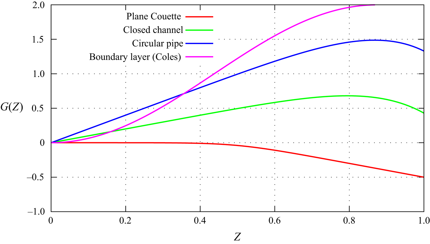
Figure 1.

Wake functions of different geometries as calculated in Luchini (Reference Luchini2018) and displayed in Luchini (Reference Luchini2019).

Whereas Panton (Reference Panton2007) extracted his representation of the wake function from a preassumed expression of the logarithmic law, and remarked that his result was sensitive to the parameter values of the latter, Luchini (Reference Luchini2018) devised a method to separate the wall and wake functions without preassuming either, based on the difference of velocity profiles at multiple Reynolds numbers in the same geometry. A lengthy examination, of all the experimental and numerical data that could be recovered at the time from the literature, led to the conclusion that a single geometry-independent wall function and three individual wake functions, respectively for pipe flow, plane-duct (closed-channel) flow and plane-Couette flow provided the best fit, in agreement with the theoretical expectation that the wall function must be universal. Analytical interpolations of such functions from Luchini (Reference Luchini2018) are collected for convenience in table 1 here. A computer implementation is available at https://CPLcode.net/Applications/FluidMechanics/TurbMeanFlow/.

Table 1.

Wall and wake functions for three classical parallel geometries.

In the overlap layer, $\ell \ll z \ll h$, these results are consistent with the asymptotic expansion proposed by Luchini (Reference Luchini2017), which extends the classical logarithmic law with a higher-order, $O(Re_\tau ^{-1})$ term in the form

(1.2)\begin{equation} u^+= \kappa^{{-}1}\log(z^+)+A_1g\,Re_\tau^{{-}1}z^++B. \end{equation}

Here $\kappa$ is von Kármán's constant, $A_1$ is a new universal constant, and the geometry parameter $g=-hp_x/\tau _w$ is related to the hydraulic diameter and takes on the fixed values of $g=2$ for circular-pipe flow, $g=1$ for plane-channel flow and $g=0$ for plane-Couette flow. Equation (1.2) stems from the ansatz that the pressure gradient $p_x$ alone (as opposed to some other feature of the outer flow) drives the first higher term in an asymptotic expansion of $u^+$ in powers of $\ell /h=Re_\tau ^{-1}$, of which the classical logarithmic law is the leading term; it is justified by the observation that, whereas other influences from the outer region can be reasonably expected to decay when $z$ becomes smaller and smaller, the pressure gradient is constant with $z$ and keeps its value all along. Relying upon the assumption of independence from $\nu$ and $h$ (which already underpins the logarithmic law) compounded with linear dependence on $p_x$, and using dimensional analysis along similar lines to Afzal & Yajnik (Reference Afzal and Yajnik1973) and Jiménez & Moser (Reference Jiménez and Moser2007), Luchini (Reference Luchini2017) determined the corrected logarithmic law to be linear in the wall-normal coordinate $z$ at first order, and eventually of the form (1.2). The best-fit values for the constants appearing in (1.2), according to Luchini (Reference Luchini2017, Reference Luchini2018), are

(1.3a–c)\begin{equation} \kappa=0.392,\quad A_1=1,\quad B=4.48, \end{equation}

respectively. When passing to the uniform representation (1.1), and recognizing that $Re_\tau ^{-1}z^+=Z$, the second term of (1.2) morphs into the first term of the Taylor expansion of $G(Z)$ in powers of $Z$, as it must do in the general theory of matched asymptotic expansions, and accordingly the wake functions reported in table 1 contain linear terms with coefficients 0, 1, 2 for respectively plane-Couette, closed-channel and circular-pipe flow. The values of the $\kappa$ and $B$ constants from (1.3a–c) also appear in the wall-function expression from table 1, thus making its large-$z^+$ behaviour consistent with (1.2).

As laid out in Luchini (Reference Luchini2018, Reference Luchini2019), the validity of the corrected logarithmic law (1.2) extends for $200\ell \lesssim z \lesssim 0.5h$, and therefore the uniform composite formula (1.1) using table 1 is an accurate representation of the complete velocity profile, well within present-day experimental and numerical error, for all $Re_\tau \gtrsim 400$. For the sake of illustration, figure 2 shows three direct numerical simulation (DNS) velocity profiles for plane-Couette, closed-channel and circular-pipe flow at $Re\simeq 1000$ compared with the corresponding predictions from table 1. Figure 3 shows the same data again, but with the logarithmic law subtracted in order to magnify their difference.

Figure 2.

Velocity profile vs wall-normal coordinate in wall units from (1.1) (solid lines) compared with numerical data (black dots), for three different geometries at $Re_\tau \simeq 1000$. The DNS data for the circular-pipe flow are taken from El Khoury et al. (Reference El Khoury, Schlatter, Noorani, Fischer, Brethouwer and Johansson2013). The DNS data for the closed-plane-duct flow are taken from Lee & Moser (Reference Lee and Moser2015). The DNS data for plane-Couette flow are taken from Pirozzoli, Bernardini & Orlandi (Reference Pirozzoli, Bernardini and Orlandi2014).

Figure 3.

Same data as figure 2, replotted as a difference to the logarithmic law.

The very good fit of velocity profiles in three different parallel geometries to (1.1) using a single wall function and wake functions that start linear in $Z$, with coefficients consistent with those geometrically derived from the corresponding pressure gradients, supports the universality of the logarithmic law and the conjecture that the pressure gradient governs its first-order correction, in addition to the general accuracy and reliability of table 1. The only visible difference to a sharp eye is a downwards displacement of approximately $-0.15$ velocity wall units between the Couette numerical simulation and its uniform representation in the central part of figure 3; but we have reason to believe that even this difference is at least partially unreal, and can be ascribed to the numerical discretization used by Pirozzoli et al. (because a similar difference can be observed in the simulation of turbulent closed-channel flow by the same numerical method in Bernardini, Pirozzoli & Orlandi Reference Bernardini, Pirozzoli and Orlandi2014). Delving into this point would lead us off topic, thus let us restrict ourselves to warning the reader that, as shown in § 7 of Luchini (Reference Luchini2018), a residual spread of order of magnitude $\pm 0.1$ is typical of today's available numerical data (including among data of different authors for the same configuration), and better than can be achieved in most experiments.

As an additional confirmation of its universality, the present wall-function formula a posteriori turned out to match remarkably well the $0\le z^+\le 200$ range of the zero-pressure gradient boundary layer of Sillero et al. (Reference Sillero, Jimenez and Moser2013), without any further fitting or tweaking (see figure 4 adapted from Luchini Reference Luchini2018). We can deduce that the wall region of a turbulent boundary layer is not just similar but practically identical to a parallel flow of the same pressure gradient, despite the outer layer being different.

Figure 4.

Comparison between the velocity profile computed in the boundary-layer DNS of Sillero, Jimenez & Moser (Reference Sillero, Jimenez and Moser2013) at momentum-thickness Reynolds number $Re_\theta =6500$ and the law of the wall from table 1, which was obtained from a fit of parallel-flow data only. Both are plotted as a difference to the logarithmic law. From figure 33 of Luchini (Reference Luchini2018).

2. Open channel

Although less thoroughly studied in the literature than the three above classical geometries, an infinite open-surface channel at zero Froude and Mach numbers is another homogeneous parallel flow that lends itself well to DNS and to the analysis techniques of Luchini (Reference Luchini2018). Sufficiently high-Reynolds DNS data for this flow have recently become available from Yao, Chen & Hussain (Reference Yao, Chen and Hussain2022).

In the limit of zero Froude number (infinite gravity) the, say water–air, open surface of a channel becomes flat (with no surface waves) and, in the additional limit of infinite density and dynamic-viscosity contrast with the overlying fluid, stress-free. Its geometry can then be schematized as a doubly infinite fluid slab of height $h$ with boundary conditions $u=v=w=0$ at $z=0$ and $u_z=v_z=w=0$ at $z=h$. In laminar flow these would also be the symmetry conditions that characterize the centreline of a closed channel with a solid wall at height $z=2h$, and the open-channel problem is therefore sometimes confused with a half-channel, but we must be wary that turbulent perturbations (contrary to the mean flow) have no mirror symmetry in a true half-channel, and are therefore different in the two cases. The turbulent mean velocity profiles of an open channel and a half-channel are nevertheless quite similar at first sight, and only identification of the wake function can critically characterize their difference.

Yao et al. (Reference Yao, Chen and Hussain2022) performed DNS of open-channel flow at $Re_\tau =180$, $550$, $1000$ and $2000$, a similar range of values as used for other geometries before them. Their mean velocity profiles, replotted here thanks to their published data files, can be seen in figure 5, with the exclusion of $Re_\tau =180$ which is too small for the present purposes. From an interpolation of these data Yao et al. derive an estimate of von Kármán's constant $\kappa =0.363$, different and in fact smaller than those inferred by other authors for closed-channel flow; they remark that a region with this approximate constant value turns up in a plot of the logarithmic derivative of the velocity profile (see figure 6) for $Re_\tau =2000$ and $500\le z^+\le 1200$, and deduce that perhaps a logarithmic region has already developed for open-channel flow at this Reynolds number, in contrast to the much higher Reynolds-number threshold believed to be necessary for a closed channel. In fairness, they also comment that high-order corrections to the logarithmic law were in the past introduced by Afzal & Yajnik (Reference Afzal and Yajnik1973) and Jiménez & Moser (Reference Jiménez and Moser2007) to better fit the mean velocity profile, and that the possibility of a universal $\kappa$ for open and closed channels as $Re_\tau \rightarrow \infty$ cannot be excluded until higher-$Re_\tau$ studies are performed. They do not seem to be specifically aware of Luchini (Reference Luchini2018).

Figure 5.

Mean velocity profiles from Yao et al. (Reference Yao, Chen and Hussain2022).

Figure 6.

Logarithmic derivative of the mean velocity profiles from Yao et al. (Reference Yao, Chen and Hussain2022).

Starting from our previous observation that the uniform representation (1.1) and the asymptotic correction (1.2) shift the asymptotic range for the validity of a logarithmic law from $Re_\tau$ greater than tens of thousands down to $Re_\tau \gtrsim 400$, here we want to explore the alternate possibility that when seen in this framework Yao et al.'s data, equipped with a suitable wake function unique to the open channel, are in fact compatible with the same universal wall function and universal von Kármán's constant as the other parallel flows summarized in § 1. If this turns out to be true, we shall at the same time quantitatively determine the wake function, which can be useful in its own right to predict open-channel velocity profiles at all other Reynolds numbers.

To this end, figure 7 displays the same data as figure 6 with the linear correction

(2.1)\begin{equation} A_1g\,Re_\tau^{{-}1}z^+ \end{equation}

(where $A_1=1$ from (1.3a–c), and $g=1$ for an open as well as for a closed channel) subtracted. As can be seen, the picture looks quite different: whereas in figure 6 the three profiles never really match, in figure 7 the $Re_\tau =1000$ and $Re_\tau =2000$ (and to a lesser degree $Re_\tau =550$) derivative profiles match one another over more than the first half of the plot. Most importantly, their common behaviour also matches the universal law of the wall from table 1, which is plotted on top of the same figure, including a fraction of the constant plateau that the latter develops for $z^+ \gtrsim 200$, with its universal value of $A_0 = 1/\kappa =2.55$. This plateau ends at $z^+\simeq 600$ for $Re_\tau =2000$ and $z^+\simeq 300$ for $Re_\tau =1000$, i.e. $z^+\simeq 0.3Re_\tau$, somewhat earlier than $z^+\simeq 0.5Re_\tau$ which was the observed upper bound for a closed channel. In contrast what in figure 6 looked like a plateau for $Re=2000$ only, has now become an oblique line which is actually part of the wake region. Most convincingly for the physical existence of the linear correction (2.1), the three separate ramps visible in figure 6 for each Reynolds number have disappeared. The top of the logarithmic region being lower also explains why $Re_\tau =550$ barely fails to fit: from equating the beginning of the logarithmic region ($z=200\ell$ as in all other geometries) to its end ($z=0.3h$ for an open channel as opposed to $z=0.5h$ for a closed one) one derives that $Re_\tau \gtrsim 666$ is here the necessary condition for an overlap logarithmic region to exist at all, whereas it was $Re_\tau \gtrsim 400$ for a closed channel.

Figure 7.

Logarithmic derivative of the mean velocity profiles from Yao et al. (Reference Yao, Chen and Hussain2022), with the linear correction (2.1) subtracted.

Once reasonable confidence has been gained that the velocity profiles for an open channel at multiple Reynolds numbers match the universal law of the wall from table 1 in its applicable range, it remains to be seen whether the remaining part of the three velocity profiles matches one and the same wake function within acceptable error for (1.1) to hold. In order to extract the shape of the wake function from (1.1) we only need to subtract the universal wall function from each velocity profile and plot the difference in outer coordinates. Such a plot is displayed in figure 8, where one should be wary that the magnified vertical scale makes errors look bigger. In reality the three wake function estimates sit within $\pm 0.1$ of each other, or $0.5\,\%$ of $u^+\approx 20$, which is the statistical variation of numerical simulations of different origins and/or different Reynolds numbers analysed by Luchini (Reference Luchini2018), and better than what can be achieved in most experiments. We believe that figure 8, combined with its resemblance to analogous plots formerly drawn for closed-duct, plane-Couette and circular-pipe flow, is sufficient evidence for the existence of a Reynolds-independent, initially linear, wake function of open-channel flow. A simple analytical interpolation of this function is proposed in table 2, and superposed to the empirically derived curves in figure 8. As further evidence that this approach can be expected to predict the velocity profile at higher Reynolds numbers, in private communication J. Yao found that his yet unpublished simulation of the open channel at $Re_\tau =4200$ is also well matched by the present formulas.

Figure 8.

Wake function estimates of the open-channel flow at different Reynolds numbers and their common analytical interpolation.

Table 2.

Wake-function interpolation for the open-channel flow.

3. Concluding remarks

After 100 years since its conception by Prandtl, the universality of the logarithmic law, of the law of the wall and of the law of the wake is still a matter of debate among scientists. Being such the situation an absolute truth can hardly be claimed, and one must confine oneself to offering arguments in favour of one or another position. Eventually Occam's razor (the philosophical principle that ‘if you have two competing ideas to explain the same phenomenon, you should prefer the simpler one’) will be our only guidance. The present author in a number of papers has been furthering arguments in favour of universality, more specifically that if the wake function is properly accounted for, and is assumed to contain a linear-in-$Z$ initial term which matches (in the sense of matched asymptotic expansions) a rational asymptotic correction to the logarithmic law, mean turbulent velocity profiles not only for different Reynolds numbers but also for different geometries collapse onto a uniform representation of the form (1.1)–(1.2).

The present paper adds the open channel to the collection of geometries that fit this framework. A coherent table containing a single universal wall function and four wake functions (one for each geometry of plane closed channel, plane Couette, circular pipe and now plane open channel) is all that is needed to provide a very accurate prediction of mean turbulent velocity profiles at all shear Reynolds numbers higher than a few hundred. We believe this table to be a valuable practical tool, and at the same time the simplest explanation currently available for such phenomena.

The interpolated wake functions of an open and closed channel are compared in figure 9. One can first of all observe that they are of the same order of magnitude and share the same initial slope, consistent with the general idea that these two flows behave similarly and have the same pressure gradient. The observation that they share their initial slope, in particular, is a strong supporting argument for the role of the pressure gradient proposed by Luchini (Reference Luchini2017) in determining such slope, since other influences such as the boundary condition at the opposite wall and even the distance to the opposite wall are obviously different in the two cases and only the pressure gradient is the same.

Figure 9.

Wake functions of open and closed channel compared.

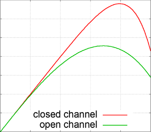
Other than this, one can observe that the wake function for the open channel is milder and peaks at a lower value than that for a closed channel, but at the same time departs earlier from its linear behaviour, which makes for a somewhat shorter range of the overlap layer. A subtler but also interesting observation is that the two wake functions exhibit different negative slopes at $Z=1$. This is unexpected because both the closed and the open channel rigorously have $u_z=0$ at $z=h$, and this condition clearly cannot be verified by the uniform representation (1.1) if the wake functions have different slopes. What actually happens, as can only be seen by looking at the horizontally magnified figure 10, is that for the open channel $u_z$ abruptly (and non-monotonically) adjusts to zero in a thin boundary layer of thickness $O(Re_\tau ^{-1})$ near the free surface. As a matter of fact (1.1) is not precisely uniformly valid for an open channel, but only so outside this thin region. Physically one should be aware that the velocity derivative approaches a non-zero limit ${\rm d}u^+/{\rm d}Z\approx 1\div 1.5$ outside this free-surface boundary layer, and in this respect closed- and open-channel flows are essentially different.

Figure 10.

Abrupt approach to zero of the velocity derivative near the upper free surface.

In closing, the wake function is of a similar order of magnitude, and should never be neglected, for an open as well as for a closed channel. Among other consequences, the open channel is just a marginally better approximation of an infinite logarithmic layer (a frequent representation of the atmospheric boundary layer) than the closed channel is. How to best simulate an infinite logarithmic layer is left as a challenge for further investigation.