


1. Introduction
Network Geometry is a rapidly developing approach in Network Science (Hoff et al., Reference Hoff, Raftery and Handcock2002] which enriches the system by modeling the nodes of the network as points in a geometric space. There are many successful examples of this approach that include latent space models (Krioukov, Reference Krioukov2016), and connections between geometry and network clustering and community structure (Gastner & Newman, Reference Gastner and Newman2006; Zuev et al., Reference Zuev, Boguná, Bianconi and Krioukov2015). Very often, these geometric embeddings naturally correspond to physical space, such as when modeling wireless networks or when networks are embedded in some geographic space (Expert et al., Reference Expert, Evans, Blondel and Lambiotte2011; Janssen, Reference Janssen2010).
Another important application of geometric graphs is in graph embeddings (Aggarwal & Murty, Reference Aggarwal and Murty2021). In order to extract useful structural information from graphs, one might want to try to embed them in a geometric space by assigning coordinates to each node such that nearby nodes are more likely to share an edge than those far from each other. Moreover, the embedding should also capture global structure and topology of the associated network, identify specific roles of nodes, etc.
Due to their spectacular successes in various applications, graph embedding methods are becoming increasingly popular in the machine learning community. They are widely used for tasks such as node classification, community detection, and link prediction, but other applications such as anomaly detection are currently explored. As reported in Chen et al. (Reference Chen, Yang, Zhang, Liu, Sun and Jin2021), the ratio between the number of papers published in top three conferences (ACL, WWW, and KDD) closely related to Computational Social Science (CSS) applying symbol-based representations and the number of papers using embeddings decreased from 10 in 2011 to 1/5 in 2020. We expect this trend to continue with embeddings eventually playing a central role in many machine learning tasks.
There are over 100 algorithms proposed in the literature for node embeddings. The techniques and possible approaches to construct the desired embedding can be broadly divided into the following three families: linear algebra algorithms, random walk-based algorithms, and deep learning methods (Aggarwal & Murty Reference Aggarwal and Murty2021; Kamiński et al., Reference Kamiński, Prałat and Théberge2022). All of these algorithms have plenty of parameters to tune, the dimension of the embedding being only one of them but an important one. Moreover, most of them are randomized algorithms which means that even for a given graph, each time we run them we get a different embedding, possibly of different quality. As a result, it is not clear which algorithm and which parameters one should use for a given application at hand. There is no clear winner and, even for the same application, the decision which algorithm to use might depend on the properties of the investigated network (Dehghan-Kooshkghazi et al., Reference Dehghan-Kooshkghazi, Kamiński, Kraiński, Prałat and Théberge2020).
In the initial version of the framework, as detailed in Kamiński et al. (Reference Kamiński, Prałat and Théberge2020), only undirected, unweighted graphs were considered. A null model was introduced by generalizing the well-known Chung–Lu model (Chung et al., Reference Chung, Chung, Graham, Lu and Chung2006) and, based on that, a global divergence score was defined. The global score can be computed for each embedding under consideration by comparing the number of edges within and between communities (obtained via some stable graph clustering algorithm) with the corresponding expected values under the null model. This global score measures how well an embedding preserves the global structure of the graph. In order to handle huge graphs, a landmark-based version of the framework was introduced in Kamiński et al. (Reference Kamiński, Prałat and Théberge2020), which can be calibrated to provide a good trade-off between performance and accuracy.
In this paper, we generalize the original framework in several ways. Firstly, we add the capability of handling both directed and undirected graphs as well as taking edge weights into account. Moreover, we introduce a new, local score which measures how well each embedding preserves local properties related to the presence of edges between pairs of nodes. The global and local scores can be combined in various ways to select good embedding(s). We illustrate the usefulness of our framework for several applications by comparing those two scores, and we show various ways to combine them to select embeddings. After appropriate adjustments to directed and/or weighted graphs, landmarks can be used the same way as in the original framework to handle huge graphs.
The paper is structured as follows. The framework is introduced in Section 2. The geometric Chung–Lu (GCL) model that is the heart of the framework is introduced and discussed in Section 3. Section 4 presents experiments justifying the usefulness of the framework and investigating the quality of a scalable approximation algorithm. Finally, some conclusions and future work are outlined in Section 5. Some extra details and experiments are available in the companion “supplementary document.”
Finally, let us mention that standard measures such as various correlations coefficients, the accuracy, and the adjusted mutual information (AMI) score are not formally defined in this paper. The reader is directed to any book on data science or machine learning (e.g. to Kamiński et al. (Reference Kamiński, Prałat and Théberge2022)) for definitions and more.
2. The framework
In this section, we introduce the unsupervised framework for comparing graph embeddings, the main contribution of this paper. Section 2.1 is devoted to high-level description and intuition behind the two embedding quality scores, local and global one, returned by the framework. The algorithm that computes them is formally defined in Section 2.2. Looking at the two scores to make an informed decision which embedding to chose is always recommended but if one wants to use the framework to select the best embedding in an unsupervised manner, then one may combine the two scores into a single value. We discuss this process in Section 2.3. The description of the scoring algorithm assumes that the graph is unweighted and directed. Generalizing it to undirected or weighted graphs is straightforward, and we discuss it in Section 2.4.
2.1 Intuition behind the algorithm
The proposed framework is multi-purposed, that is, it independently evaluates embeddings using two approaches.
The first approach looks at the network and the associated embeddings “from the distance,” trying to see a “big picture.” It evaluates the embeddings based on their ability to capture global properties of the network, namely, edge densities. In order to achieve it, the framework compares edge density between and within the communities that are present (and can be easily recovered) in the evaluated graph $G$
with the corresponding expected edge density in the associated random null model. This score is designed to identify embeddings that should perform well in tasks requiring global knowledge of the graph such as node classification or community detection. We will call this measure a global score.
$G$
with the corresponding expected edge density in the associated random null model. This score is designed to identify embeddings that should perform well in tasks requiring global knowledge of the graph such as node classification or community detection. We will call this measure a global score.
The second approach looks at the network and embeddings “under the microscope,” trying to see if a local structure of a graph $G$
is well reflected by the associated embedding. The local score will be designed in such a way that it is able to evaluate if the embedding is a strong predictor of (directed) adjacency between nodes in the network. In general, this property could be tested using any strong supervised machine learning algorithm. However, our objective is to test not only predictive power but also explainability of the embedding (sometimes referred to as interpretability). Namely, we assume that the adjacency probability between nodes should be monotonically linked with their distance in the embedding and their in and out degrees. This approach has the following advantage: embeddings that score well should not only be useful for link prediction, but they should perform well in any task that requires a local knowledge of the graph. To achieve this, we use the same random null model as we use to calculate the global score to estimate the probability of two nodes to be adjacent. This question is the well-known and well-studied problem of link prediction in which one seeks to find the node pairs most likely to be linked by an edge. When computing the local score, we calculate a ranking of the node pairs from most to least likely of being linked. A common evaluation method for such problem is to compute the AUC (area under the ROC curve). It is important to note that the AUC is independent of the ratio between the number of edges and the number of non-edges in the graph. As a result, it can be approximated using random sampling.
$G$
is well reflected by the associated embedding. The local score will be designed in such a way that it is able to evaluate if the embedding is a strong predictor of (directed) adjacency between nodes in the network. In general, this property could be tested using any strong supervised machine learning algorithm. However, our objective is to test not only predictive power but also explainability of the embedding (sometimes referred to as interpretability). Namely, we assume that the adjacency probability between nodes should be monotonically linked with their distance in the embedding and their in and out degrees. This approach has the following advantage: embeddings that score well should not only be useful for link prediction, but they should perform well in any task that requires a local knowledge of the graph. To achieve this, we use the same random null model as we use to calculate the global score to estimate the probability of two nodes to be adjacent. This question is the well-known and well-studied problem of link prediction in which one seeks to find the node pairs most likely to be linked by an edge. When computing the local score, we calculate a ranking of the node pairs from most to least likely of being linked. A common evaluation method for such problem is to compute the AUC (area under the ROC curve). It is important to note that the AUC is independent of the ratio between the number of edges and the number of non-edges in the graph. As a result, it can be approximated using random sampling.
Despite the fact that the global and local scores take diametrically different points of view, there is often correlation between the two. Good embeddings tend to capture both global and local properties and, as a result, they score well in both approaches. On the other hand, poor embeddings have problems with capturing any useful properties of graphs and so their corresponding scores are both bad. Nevertheless, they are certainly not identical, and we will show examples in which the two scores are different.
2.2 The algorithm
In this section, and later in the paper, we use $[n]$
to denote the set of natural numbers less than or equal to
$[n]$
to denote the set of natural numbers less than or equal to $n$
, that is,
$n$
, that is, $[n] \;:\!=\; \{1, \ldots, n\}$
. Given a directed graph
$[n] \;:\!=\; \{1, \ldots, n\}$
. Given a directed graph $G=(V,E)$
(in particular, given its in-degree and out-degree distributions
$G=(V,E)$
(in particular, given its in-degree and out-degree distributions $\textbf{w}^{in}$
and
$\textbf{w}^{in}$
and $\textbf{w}^{out}$
on
$\textbf{w}^{out}$
on $V$
) and an embedding
$V$
) and an embedding $\mathcal E : V \to{\mathbb R}^k$
of its nodes in
$\mathcal E : V \to{\mathbb R}^k$
of its nodes in $k$
-dimensional space, we perform the steps detailed below to obtain
$k$
-dimensional space, we perform the steps detailed below to obtain $(\Delta _{\mathcal E}^{g}(G),\Delta _{\mathcal E}^{\ell }(G))$
, a pair of respectively global and local divergence scores for the embedding. Indeed, as already mentioned the framework is multi-purposed and, depending on the specific application in mind, one might want the selected embeddings that preserve global properties (density-based evaluation) and/or pay attention to local properties (link-based evaluation). As a result, we independently compute the two corresponding divergence scores,
$(\Delta _{\mathcal E}^{g}(G),\Delta _{\mathcal E}^{\ell }(G))$
, a pair of respectively global and local divergence scores for the embedding. Indeed, as already mentioned the framework is multi-purposed and, depending on the specific application in mind, one might want the selected embeddings that preserve global properties (density-based evaluation) and/or pay attention to local properties (link-based evaluation). As a result, we independently compute the two corresponding divergence scores, $\Delta ^{g}_{\mathcal E_i}(G)$
and
$\Delta ^{g}_{\mathcal E_i}(G)$
and $\Delta ^{\ell }_{\mathcal E_i}(G)$
, to provide the users of the framework with a more complete picture and let them make an informative decision which embedding to use. We typically apply this algorithm to compare several embeddings
$\Delta ^{\ell }_{\mathcal E_i}(G)$
, to provide the users of the framework with a more complete picture and let them make an informative decision which embedding to use. We typically apply this algorithm to compare several embeddings $\mathcal E_1,\ldots,\mathcal E_m$
of the same graph and select the best one via
$\mathcal E_1,\ldots,\mathcal E_m$
of the same graph and select the best one via $\text{argmin}_{i\in [m]} \Delta _{\mathcal E_i}(G)$
, where
$\text{argmin}_{i\in [m]} \Delta _{\mathcal E_i}(G)$
, where $\Delta _{\mathcal E_i}(G)$
is the combined divergence score that takes into account the scores of the competitors and that can be tuned for a given application at hand.
$\Delta _{\mathcal E_i}(G)$
is the combined divergence score that takes into account the scores of the competitors and that can be tuned for a given application at hand.
Note that our algorithm is a general framework, and some parts have flexibility. We clearly identify these below and provide a specific, default, approach that we applied in our implementation. In the description below, we assume that the graph is directed and unweighted, and we then discuss how the framework deals with undirected and/or weighted graphs.
The code can be accessed at the GitHub repositoryFootnote 1. The first version of the framework (c.f. Kamiński et al. (Reference Kamiński, Prałat and Théberge2020)) was designed for undirected, unweighted graphs, and only used the density-based evaluation. Since it was used for experiments reported in various papers, for reproducibility purpose, the code can still be accessed on GitHubFootnote 2.
2.2.1 Global (Density-based) evaluation: $\Delta ^{g}_{\mathcal E}(G)$

Step 1: Run some stable graph clustering algorithm on $G$
to obtain a partition
$G$
to obtain a partition $\textbf{C}$
of the set of nodes
$\textbf{C}$
of the set of nodes $V$
into
$V$
into $\ell$
communities
$\ell$
communities $C_1, \ldots, C_\ell$
.
$C_1, \ldots, C_\ell$
.
Note: In our implementation, we used the ensemble clustering algorithm for unweighted graphs (ECG) which is based on the Louvain algorithm (Blondel et al., Reference Blondel, Guillaume, Lambiotte and Lefebvre2008) and the concept of consensus clustering (Poulin & Théberge Reference Poulin and Théberge2018) and is shown to have good stability. For weighted graphs, by default we use the Louvain algorithm.
Note: In some applications, the desired partition may be provided together with a graph (e.g., when nodes contain some natural labeling and so some form of a ground-truth is provided). The framework is flexible and allows for communities to be provided as an input to the framework instead of using a clustering algorithm. In the supplementary document, we present a number of experiments that show that the choice of clustering algorithm does not affect the score in a significant way (provided the clustering is stable and of good quality).
Step 2: For each $i \in [\ell ]$
, let
$i \in [\ell ]$
, let $c_{i}$
be the proportion of directed edges of
$c_{i}$
be the proportion of directed edges of $G$
with both end points in
$G$
with both end points in $C_i$
. Similarly, for each
$C_i$
. Similarly, for each $1 \le i, j \le \ell$
,
$1 \le i, j \le \ell$
, $i \neq j$
, let
$i \neq j$
, let $c_{i,j}$
be the proportion of directed edges of
$c_{i,j}$
be the proportion of directed edges of $G$
from some node in
$G$
from some node in $C_i$
to some node in
$C_i$
to some node in $C_j$
. Let
$C_j$
. Let
 \begin{align} \bar{\textbf{c}} &= (c_{1,2},c_{2,1},\ldots, c_{1,\ell }, c_{\ell,1}, c_{2,3}, c_{3,2}, \ldots, c_{\ell -1,\ell }, c_{\ell,\ell -1} ) \nonumber \\[5pt] \hat{\textbf{c}} &= (c_1, \ldots, c_\ell ) \end{align}
and let $\textbf{c} = \bar{\textbf{c}} \oplus \hat{\textbf{c}}$
be the concatenation of the two vectors with a total of
$\textbf{c} = \bar{\textbf{c}} \oplus \hat{\textbf{c}}$
be the concatenation of the two vectors with a total of $2 \binom{\ell }{2} + \ell = \ell ^2$
entries which together sum to one. This graph vector
$2 \binom{\ell }{2} + \ell = \ell ^2$
entries which together sum to one. This graph vector $\textbf{c}$
characterizes the partition
$\textbf{c}$
characterizes the partition $\textbf{C}$
from the perspective of the graph
$\textbf{C}$
from the perspective of the graph $G$
.
$G$
.
Note: The embedding $\mathcal E$
does not affect the vectors
$\mathcal E$
does not affect the vectors $\bar{\textbf{c}}$
and
$\bar{\textbf{c}}$
and $\hat{\textbf{c}}$
(and so also
$\hat{\textbf{c}}$
(and so also $\textbf{c}$
). They are calculated purely based on
$\textbf{c}$
). They are calculated purely based on $G$
and the partition
$G$
and the partition $\textbf{C}$
.
$\textbf{C}$
.
Step 3: For a given parameter $\alpha \in{\mathbb R}_+$
and the same partition of nodes
$\alpha \in{\mathbb R}_+$
and the same partition of nodes $\textbf{C}$
, we consider the GCL directed graph model
$\textbf{C}$
, we consider the GCL directed graph model $\mathcal{G}(\textbf{w}^{in}, \textbf{w}^{out}, \mathcal E, \alpha )$
presented in Section 3 that can be viewed in this context as the associated null model. For each
$\mathcal{G}(\textbf{w}^{in}, \textbf{w}^{out}, \mathcal E, \alpha )$
presented in Section 3 that can be viewed in this context as the associated null model. For each $1 \le i, j \le \ell$
,
$1 \le i, j \le \ell$
, $i \neq j$
, we compute
$i \neq j$
, we compute $b_{i,j}$
, the expected proportion of directed edges of
$b_{i,j}$
, the expected proportion of directed edges of $\mathcal{G}(\textbf{w}^{in}, \textbf{w}^{out}, \mathcal E, \alpha )$
from some node in
$\mathcal{G}(\textbf{w}^{in}, \textbf{w}^{out}, \mathcal E, \alpha )$
from some node in $C_i$
to some node in
$C_i$
to some node in $C_j$
. Similarly, for each
$C_j$
. Similarly, for each $i \in [\ell ]$
, let
$i \in [\ell ]$
, let $b_i$
be the expected proportion of directed edges within
$b_i$
be the expected proportion of directed edges within $C_i$
. That gives us another two vectors:
$C_i$
. That gives us another two vectors:
 \begin{align} \bar{\textbf{b}}_{\mathcal E}(\alpha ) &= (b_{1,2}, b_{2,1}, \ldots, b_{1,\ell }, b_{\ell,1}, b_{2,3}, b_{3,2}, \ldots, b_{\ell -1,\ell }, b_{\ell,\ell -1} ) \nonumber \\[5pt] \hat{\textbf{b}}_{\mathcal E}(\alpha ) &= (b_{1},\ldots, b_{\ell } ) \end{align}
and let $\textbf{b}_{\mathcal E}(\alpha ) = \bar{\textbf{b}}_{\mathcal E}(\alpha ) \oplus \hat{\textbf{b}}_{\mathcal E}(\alpha )$
be the concatenation of the two vectors with a total of
$\textbf{b}_{\mathcal E}(\alpha ) = \bar{\textbf{b}}_{\mathcal E}(\alpha ) \oplus \hat{\textbf{b}}_{\mathcal E}(\alpha )$
be the concatenation of the two vectors with a total of $\ell ^2$
entries which together sum to one. This model vector
$\ell ^2$
entries which together sum to one. This model vector $\textbf{b}_{\mathcal E}(\alpha )$
characterizes the partition
$\textbf{b}_{\mathcal E}(\alpha )$
characterizes the partition $\textbf{C}$
from the perspective of the embedding
$\textbf{C}$
from the perspective of the embedding $\mathcal E$
.
$\mathcal E$
.
Note: The structure of graph $G$
does not affect the vectors
$G$
does not affect the vectors $\bar{\textbf{b}}_{\mathcal E}(\alpha )$
and
$\bar{\textbf{b}}_{\mathcal E}(\alpha )$
and $\hat{\textbf{b}}_{\mathcal E}(\alpha )$
; only its degree distribution
$\hat{\textbf{b}}_{\mathcal E}(\alpha )$
; only its degree distribution $\textbf{w}^{in}$
,
$\textbf{w}^{in}$
, $\textbf{w}^{out}$
, and embedding
$\textbf{w}^{out}$
, and embedding $\mathcal E$
are used.
$\mathcal E$
are used.
Note: We used the GCL directed graph model, but the framework is flexible. If, for any reason (perhaps there are some restrictions for the maximum edge length; such restrictions are often present in, for example, wireless networks) it makes more sense to use some other model of random geometric graphs, it can be easily implemented here. If the model is too complicated and computing the expected number of edges between two parts is challenging, then it can be approximated via simulations.
Step 4: Compute the distance $\Delta _\alpha$
between the two vectors,
$\Delta _\alpha$
between the two vectors, $\textbf{c}$
and
$\textbf{c}$
and $\textbf{b}_{\mathcal E}(\alpha )$
, in order to measure how well the model
$\textbf{b}_{\mathcal E}(\alpha )$
, in order to measure how well the model $\mathcal{G}(\textbf{w}^{in}, \textbf{w}^{out}, \mathcal E, \alpha )$
fits the graph
$\mathcal{G}(\textbf{w}^{in}, \textbf{w}^{out}, \mathcal E, \alpha )$
fits the graph $G$
.
$G$
.
Note: We used the well-known and widely used Jensen–Shannon divergence (JSD) to measure the dissimilarity between two probability distributions, that is, $\Delta _\alpha = JSD(\textbf{c},\textbf{b}_{\mathcal E}(\alpha ))$
. The JSD was originally proposed in Lin (Reference Lin1991) and can be viewed as a smoothed version of the Kullback–Leibler divergence.
$\Delta _\alpha = JSD(\textbf{c},\textbf{b}_{\mathcal E}(\alpha ))$
. The JSD was originally proposed in Lin (Reference Lin1991) and can be viewed as a smoothed version of the Kullback–Leibler divergence.
Note: Alternatively, one may independently treat internal and external edges to compensate the fact that there are $2 \binom{\ell }{2} = \Theta (\ell ^2)$
coefficients related to external densities, whereas only
$2 \binom{\ell }{2} = \Theta (\ell ^2)$
coefficients related to external densities, whereas only $\ell$
ones related to internal ones. Then, for example, after appropriate normalization of the vectors, a simple average of the two corresponding distances can be used, that is,
$\ell$
ones related to internal ones. Then, for example, after appropriate normalization of the vectors, a simple average of the two corresponding distances can be used, that is,
 \begin{equation*} \Delta _\alpha = \frac 12 \cdot \left ( JSD(\bar {\bf c},\bar {\bf b}_{\mathcal E}(\alpha )) + JSD(\hat {\bf c},\hat {\bf b}_{\mathcal E}(\alpha )) \right ) \end{equation*}
Depending on the application at hand, other weighted averages can be used if more weight needs to be put on internal or external edges.
Step 5: Select $\hat{\alpha } = \text{argmin}_{\alpha } \Delta _\alpha$
and define the global (density-based) score for embedding
$\hat{\alpha } = \text{argmin}_{\alpha } \Delta _\alpha$
and define the global (density-based) score for embedding $\mathcal E$
on
$\mathcal E$
on $G$
as
$G$
as $\Delta _{\mathcal E}^g(G) = \Delta _{\hat{\alpha }}$
.
$\Delta _{\mathcal E}^g(G) = \Delta _{\hat{\alpha }}$
.
Note: The parameter $\alpha$
is used to define a distance in the embedding space, as we detail in Section 3. In our implementation, we simply checked values of
$\alpha$
is used to define a distance in the embedding space, as we detail in Section 3. In our implementation, we simply checked values of $\alpha$
from a dense grid, starting from
$\alpha$
from a dense grid, starting from $\alpha =0$
and finishing the search if no improvement is found for five consecutive values of
$\alpha =0$
and finishing the search if no improvement is found for five consecutive values of $\alpha$
. Clearly, there are potentially faster ways to find an optimum value of
$\alpha$
. Clearly, there are potentially faster ways to find an optimum value of $\alpha$
but, since our algorithm is the fast-performing grid search, this approach was chosen as both easy to implement and robust to potential local optima.
$\alpha$
but, since our algorithm is the fast-performing grid search, this approach was chosen as both easy to implement and robust to potential local optima.
2.2.2 Local (Link-based) evaluation:
$\Delta _{\mathcal E}^{\ell }(G)$

Step 6: We let
 \begin{align*} S^+ &= \{ (u, v) \in V \times V, u \ne v ;\; uv \in E \}, \\[5pt] S^- &= \{ (u, v) \in V \times V, u \ne v ;\; uv \notin E \}. \end{align*}
For a given parameter $\alpha \in{\mathbb R}_+$
, we again consider the GCL directed graph model
$\alpha \in{\mathbb R}_+$
, we again consider the GCL directed graph model $\mathcal{G}(\textbf{w}^{in}, \textbf{w}^{out}, \mathcal E, \alpha )$
detailed in Section 3. Let
$\mathcal{G}(\textbf{w}^{in}, \textbf{w}^{out}, \mathcal E, \alpha )$
detailed in Section 3. Let $p(u,v)$
be the probability of a directed edge
$p(u,v)$
be the probability of a directed edge $u \rightarrow v$
to be present under this model.
$u \rightarrow v$
to be present under this model.
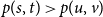
The receiver operating characteristic (ROC) is a curve showing the performance of a classification model at all classification thresholds (for the edge probabilities in the present context). The AUC (area under the ROC curve) provides an aggregate measure of performance across all possible classification thresholds which can be interpreted as the probability that a randomly chosen positive sample (here, a pair of nodes connected by an edge) is ranked higher that a negative sample (a pair of nodes without an edge). Thus, the AUC can be expressed as follows:
 \begin{equation*} p_\alpha = \frac {\sum _{(s,t) \in S^+} \sum _{(u,v) \in S^-} \mathbb {1}{\{ p(s,t) \gt p(u,v) \}}}{|S^+| \cdot |S^-|} \end{equation*}
As a result, the AUC measures how much the model is capable of distinguishing between the two classes, $S^+$
and
$S^+$
and $S^-$
. In other words, it may be viewed as the probability that
$S^-$
. In other words, it may be viewed as the probability that $p(s,t) \gt p(u,v)$
, provided that a directed edge
$p(s,t) \gt p(u,v)$
, provided that a directed edge $s \rightarrow t$
and a directed non-edge
$s \rightarrow t$
and a directed non-edge $u \not \rightarrow v$
are selected uniformly at random from
$u \not \rightarrow v$
are selected uniformly at random from $S^+$
and, respectively,
$S^+$
and, respectively, $S^-$
.
$S^-$
.
Note: In practice, there is no need to investigate all $|S^+| \cdot |S^-|$
pairs of nodes. Instead, we can randomly sample (with replacement)
$|S^+| \cdot |S^-|$
pairs of nodes. Instead, we can randomly sample (with replacement) $k$
pairs
$k$
pairs $(s_i,t_i) \in S^+$
and
$(s_i,t_i) \in S^+$
and $k$
pairs
$k$
pairs $(u_i,v_i) \in S^-$
and then compute
$(u_i,v_i) \in S^-$
and then compute
 \begin{equation*} \hat {p}_\alpha = \frac {\sum _{i=1}^k \mathbb {1}{\{ p(s_i,t_i) \gt p(u_i,v_i) \}}}{k} \end{equation*}
to approximate $p_\alpha$
. The value of
$p_\alpha$
. The value of $k$
is adjusted so that the approximate 95% confidence interval, namely,
$k$
is adjusted so that the approximate 95% confidence interval, namely,
 \begin{equation*} \left [ \hat {p}_\alpha - 1.96 \sqrt {\hat {p}_\alpha (1-\hat {p}_\alpha )/k}, \hat {p}_\alpha + 1.96 \sqrt {\hat {p}_\alpha (1-\hat {p}_\alpha )/k} \right ] \end{equation*}
is shorter that some precision level. In our implementation, the default value of $k$
is set to
$k$
is set to $k=10{,}000$
so that the length of the interval is guaranteed to be at most
$k=10{,}000$
so that the length of the interval is guaranteed to be at most $0.02$
.
$0.02$
.
Step 7: Select $\hat{\alpha } = \text{argmin}_{\alpha } (1-\hat{p}_\alpha )$
and define the local (link-based) score for embedding
$\hat{\alpha } = \text{argmin}_{\alpha } (1-\hat{p}_\alpha )$
and define the local (link-based) score for embedding $\mathcal E$
on
$\mathcal E$
on $G$
as
$G$
as $\Delta _{\mathcal E}^{\ell }(G) = 1-\hat{p}_{\hat{\alpha }}$
.
$\Delta _{\mathcal E}^{\ell }(G) = 1-\hat{p}_{\hat{\alpha }}$
.
2.3 Combined divergence scores for evaluating many embeddings
As already mentioned a few times, the framework is multi-purposed and, depending on the specific application in mind, one might want the selected embeddings that preserve global properties (global, density-based evaluation) or pay more attention to local properties (local, link-based evaluation). That is the reason, we independently compute the two corresponding divergence scores, $\Delta ^{g}_{\mathcal E_i}(G)$
and
$\Delta ^{g}_{\mathcal E_i}(G)$
and $\Delta ^{\ell }_{\mathcal E_i}(G)$
.
$\Delta ^{\ell }_{\mathcal E_i}(G)$
.
In order to compare several embeddings for the same graph $G$
, we repeat steps 3–7 above, each time computing the two scores for a given embedding. Let us stress again that steps 1–2 are done only once, that is, we use the same partition of the graph into
$G$
, we repeat steps 3–7 above, each time computing the two scores for a given embedding. Let us stress again that steps 1–2 are done only once, that is, we use the same partition of the graph into $\ell$
communities for all embeddings. In order to select (in an unsupervised way) the best embedding to be used, one may simply compute the combined divergence score, a linear combination of the two scores:
$\ell$
communities for all embeddings. In order to select (in an unsupervised way) the best embedding to be used, one may simply compute the combined divergence score, a linear combination of the two scores:
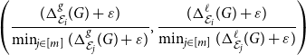
 \begin{equation} \Delta _{\mathcal E_i}(G) = q \cdot \frac{ (\Delta ^{g}_{\mathcal E_i}(G) + \varepsilon ) }{ \min _{j \in [m]} ( \Delta ^{g}_{\mathcal E_j}(G) + \varepsilon ) } + (1-q) \cdot \frac{ (\Delta ^{\ell }_{\mathcal E_i}(G) + \varepsilon ) }{\min _{j \in [m]} ( \Delta ^{\ell }_{\mathcal E_j}(G) + \varepsilon ) } \end{equation}
for a fixed parameter $q \in [0,1]$
, carefully selected for a given application at hand, and
$q \in [0,1]$
, carefully selected for a given application at hand, and $\varepsilon =0.01$
, introduced to prevent rare but possible numerical issues when one of the scores is close to zero. Note that
$\varepsilon =0.01$
, introduced to prevent rare but possible numerical issues when one of the scores is close to zero. Note that $\Delta _{\mathcal E_i}(G) \ge 1$
and
$\Delta _{\mathcal E_i}(G) \ge 1$
and $\Delta _{\mathcal E_i}(G) = 1$
if and only if a given embedding
$\Delta _{\mathcal E_i}(G) = 1$
if and only if a given embedding $\mathcal E_i$
does not have a better competitor in any of the two evaluation criteria. Of course, the lower the score, the better the embedding is. The winner
$\mathcal E_i$
does not have a better competitor in any of the two evaluation criteria. Of course, the lower the score, the better the embedding is. The winner $\mathcal E_j$
can be identified by taking
$\mathcal E_j$
can be identified by taking $j = \text{argmin}_i \Delta _{\mathcal E_i}(G)$
.
$j = \text{argmin}_i \Delta _{\mathcal E_i}(G)$
.
Let us briefly justify the choice of function (3). First note that both $\Delta ^{g}_{\mathcal E_i}(G)$
and
$\Delta ^{g}_{\mathcal E_i}(G)$
and $\Delta ^{\ell }_{\mathcal E_i}(G)$
are in
$\Delta ^{\ell }_{\mathcal E_i}(G)$
are in $[0,1]$
. However, since they might have different orders of magnitude (and typically they do), the corresponding scores need to be normalized. In decision theory, one typically simply tunes
$[0,1]$
. However, since they might have different orders of magnitude (and typically they do), the corresponding scores need to be normalized. In decision theory, one typically simply tunes $q$
to properly take this into account. While we allow for the more advanced user to change the value of
$q$
to properly take this into account. While we allow for the more advanced user to change the value of $q$
, we believe that it is preferable to provide a reasonable scaling when the default value of
$q$
, we believe that it is preferable to provide a reasonable scaling when the default value of $q$
, namely,
$q$
, namely, $q=1/2$
is used. When choosing a normalization by minimum, we were guided by the fact that it is not uncommon that most of the embeddings score poorly in both dimensions; if this is so, then they affect for example the average score but they ideally should not influence the selection process. On the other hand, the minimum clearly should not be affected by bad embeddings. In particular, the normalization by the minimum allows us to distinguish the situation in which two embeddings have similar but large scores (indicating that both embeddings are bad) from the situation in which two embeddings have similar but small scores (one of the two corresponding embeddings can still be significantly better).
$q=1/2$
is used. When choosing a normalization by minimum, we were guided by the fact that it is not uncommon that most of the embeddings score poorly in both dimensions; if this is so, then they affect for example the average score but they ideally should not influence the selection process. On the other hand, the minimum clearly should not be affected by bad embeddings. In particular, the normalization by the minimum allows us to distinguish the situation in which two embeddings have similar but large scores (indicating that both embeddings are bad) from the situation in which two embeddings have similar but small scores (one of the two corresponding embeddings can still be significantly better).
Finally, let us mention that while having a single score assigned to each embedding is useful, it is always better to look at the composition of the scores,
 \begin{equation*} \left ( \frac { (\Delta ^{g}_{\mathcal E_i}(G) + \varepsilon ) } { \min _{j \in [m]} (\Delta ^{g}_{\mathcal E_j}(G) + \varepsilon ) }, \frac { (\Delta ^{\ell }_{\mathcal E_i}(G) + \varepsilon ) } {\min _{j \in [m]} (\Delta ^{\ell }_{\mathcal E_j}(G) + \varepsilon ) } \right ) \end{equation*}
to make a more informative decision. See Section 4.3 for an example of such a selection process.
2.4 Weighted and undirected graphs
For simplicity, we defined the framework for unweighted but directed graphs. Extending the density-based evaluation to weighted graphs can be easily and naturally done by considering the sum of weights of the edges instead of the number of them, for example, $c_i$
is the proportion of the total weight concentrated on the directed edges with both end points in
$c_i$
is the proportion of the total weight concentrated on the directed edges with both end points in $C_i$
. For the link-based evaluation, we need to adjust the definition of the AUC so that it is equal to the probability that
$C_i$
. For the link-based evaluation, we need to adjust the definition of the AUC so that it is equal to the probability that $p(s,t) \gt p(u,v)$
times the weight of a directed edge
$p(s,t) \gt p(u,v)$
times the weight of a directed edge $s \rightarrow t$
(scaled appropriately such that the average scaled weight of all edges investigated is equal to one), provided that a directed edge
$s \rightarrow t$
(scaled appropriately such that the average scaled weight of all edges investigated is equal to one), provided that a directed edge $s \rightarrow t$
is selected from
$s \rightarrow t$
is selected from $S^+$
(the set of all edges) and a directed non-edge
$S^+$
(the set of all edges) and a directed non-edge $u \not \rightarrow v$
is selected from
$u \not \rightarrow v$
is selected from $S^-$
(the set of non-edges), both of them uniformly at random. As before, such quantity may be efficiently approximated by sampling.
$S^-$
(the set of non-edges), both of them uniformly at random. As before, such quantity may be efficiently approximated by sampling.
On the other hand, clearly undirected graphs can be viewed as directed ones by replacing each undirected edge $uv$
by two directed edges
$uv$
by two directed edges $uv$
and
$uv$
and $vu$
. Hence, one can transform an undirected graph
$vu$
. Hence, one can transform an undirected graph $G$
to its directed counterpart and run the framework on it. However, the framework is tuned for a faster running time when undirected graphs are used but, of course, the divergence score remains unaffected.
$G$
to its directed counterpart and run the framework on it. However, the framework is tuned for a faster running time when undirected graphs are used but, of course, the divergence score remains unaffected.
3. GCL model
The heart of the framework is the associated random graph null model that is used to design both the global and the local score. The GCL model, a generalization of the original Chung–Lu model (Chung et al., Reference Chung, Chung, Graham, Lu and Chung2006), was introduced in Kamiński et al. (Reference Kamiński, Prałat and Théberge2020) to benchmark embeddings of undirected graphs (at that time only from the global perspective). Now, we need to generalize it even further to include directed and weighted graphs. We do it in Section 3.1. A scalable implementation in discussed in Section 3.2.
3.1 Geometric directed model
In the GCL directed graph model, we are not only given the expected degree distribution of a directed graph $G$
$G$
 \begin{align*} \textbf{w}^{in} &= (w_1^{in}, \ldots, w_n^{in}) = (\deg ^{in}_G(v_1), \ldots, \deg ^{in}_G(v_n)) \\[5pt] \textbf{w}^{out} &= (w_1^{out}, \ldots, w_n^{out}) = (\deg ^{out}_G(v_1), \ldots, \deg ^{out}_G(v_n)) \end{align*}
but also an embedding $\mathcal E$
of nodes of
$\mathcal E$
of nodes of $G$
in some
$G$
in some $k$
-dimensional space,
$k$
-dimensional space, $\mathcal E : V \to{\mathbb R}^k$
. In particular, for each pair of nodes,
$\mathcal E : V \to{\mathbb R}^k$
. In particular, for each pair of nodes, $v_i$
,
$v_i$
, $v_j$
, we know the distance between them:
$v_j$
, we know the distance between them:
 \begin{equation*} d_{i,j} = \textrm {dist}( \mathcal E(v_i), \mathcal E(v_j)) \end{equation*}
It is desired that the probability that nodes $v_i$
and
$v_i$
and $v_j$
are adjacent to be a function of
$v_j$
are adjacent to be a function of $d_{i,j}$
, that is, to be proportional to
$d_{i,j}$
, that is, to be proportional to $g(d_{i,j})$
for some function
$g(d_{i,j})$
for some function $g$
. The function
$g$
. The function $g$
should be a decreasing function as long edges should occur less frequently than short ones. There are many natural choices such as
$g$
should be a decreasing function as long edges should occur less frequently than short ones. There are many natural choices such as $g(d) = d^{-\beta }$
for some
$g(d) = d^{-\beta }$
for some $\beta \in [0, \infty )$
or
$\beta \in [0, \infty )$
or $g(d) = \exp (-\gamma d)$
for some
$g(d) = \exp (-\gamma d)$
for some $\gamma \in [0, \infty )$
. We use the following, normalized function
$\gamma \in [0, \infty )$
. We use the following, normalized function $g:[0,\infty ) \to [0,1]$
: for a fixed
$g:[0,\infty ) \to [0,1]$
: for a fixed $\alpha \in [0,\infty )$
, let
$\alpha \in [0,\infty )$
, let
 \begin{equation*} g(d) \;:\!=\; \left ( 1 - \frac {d - d_{\min }}{d_{\max } - d_{\min }} \right )^{\alpha } = \left ( \frac {d_{\max } - d}{d_{\max } - d_{\min }} \right )^{\alpha } \end{equation*}
where
 \begin{align*} d_{\min } &= \min \{ \textrm{dist}(\mathcal E(v), \mathcal E(w))\;:\; v,w \in V, v\neq w\} \\[5pt] d_{\max } &= \max \{ \textrm{dist}(\mathcal E(v), \mathcal E(w))\;:\; v,w \in V \} \end{align*}
are the minimum, and respectively the maximum, distance between nodes in embedding $\mathcal E$
. One convenient and desired property of this function is that it is invariant with respect to an affine transformation of the distance measure. Clearly,
$\mathcal E$
. One convenient and desired property of this function is that it is invariant with respect to an affine transformation of the distance measure. Clearly, $g(d_{\min })=1$
and
$g(d_{\min })=1$
and $g(d_{\max })=0$
; in the computations, we can use clipping to force
$g(d_{\max })=0$
; in the computations, we can use clipping to force $g(d_{\min })\lt 1$
and/or
$g(d_{\min })\lt 1$
and/or $g(d_{\max })\gt 0$
if required. Let us also note that if
$g(d_{\max })\gt 0$
if required. Let us also note that if $\alpha = 0$
(that is,
$\alpha = 0$
(that is, $g(d)=1$
for any
$g(d)=1$
for any $d \in [d_{\min },d_{\max })$
with the convention that
$d \in [d_{\min },d_{\max })$
with the convention that $g(d_{\max })=0^0=1$
), then the pairwise distances are neglected. As a result, in particular, for undirected graphs we recover the original Chung–Lu model. Moreover, the larger parameter
$g(d_{\max })=0^0=1$
), then the pairwise distances are neglected. As a result, in particular, for undirected graphs we recover the original Chung–Lu model. Moreover, the larger parameter $\alpha$
is, the larger the aversion to long edges is. Since this family of functions (for various values of the parameter
$\alpha$
is, the larger the aversion to long edges is. Since this family of functions (for various values of the parameter $\alpha$
) captures a wide spectrum of behaviors, it should be enough to concentrate on this choice, but one can experiment with other functions. So, for now we may assume that the only parameter of the model is
$\alpha$
) captures a wide spectrum of behaviors, it should be enough to concentrate on this choice, but one can experiment with other functions. So, for now we may assume that the only parameter of the model is $\alpha \in [0,\infty )$
.
$\alpha \in [0,\infty )$
.
The GCL directed graph model is the random graph $G(\textbf{w}^{in}, \textbf{w}^{out}, \mathcal E, \alpha )$
on the set of nodes
$G(\textbf{w}^{in}, \textbf{w}^{out}, \mathcal E, \alpha )$
on the set of nodes $V = \{ v_1, \ldots, v_n \}$
in which each pair of nodes
$V = \{ v_1, \ldots, v_n \}$
in which each pair of nodes $v_i, v_j$
, independently of other pairs, forms a directed edge from
$v_i, v_j$
, independently of other pairs, forms a directed edge from $v_i$
to
$v_i$
to $v_j$
with probability
$v_j$
with probability $p_{i,j}$
, where
$p_{i,j}$
, where
 \begin{equation*} p_{i,j} = x_i^{out} x_j^{in} g(d_{i,j}) \end{equation*}
for some carefully tuned weights $x_i^{in}, x_i^{out} \in{\mathbb R}_+$
. The weights are selected such that the expected in-degree and out-degree of
$x_i^{in}, x_i^{out} \in{\mathbb R}_+$
. The weights are selected such that the expected in-degree and out-degree of $v_i$
is
$v_i$
is $w_i^{in}$
and, respectively,
$w_i^{in}$
and, respectively, $w_i^{out}$
; that is, for all
$w_i^{out}$
; that is, for all $i \in [n]$
 \begin{align*} w_i^{out} &= \sum _{j \in [n], j\neq i} p_{i,j} = x_i^{out} \sum _{j \in [n], j\neq i} x_j^{in} g(d_{i,j}) \\[5pt] w_i^{in} &= \sum _{j \in [n], j\neq i} p_{j,i} = x_i^{in} \sum _{j \in [n], j\neq i} x_j^{out} g(d_{i,j}) \end{align*}
Additionally, we set $p_{i,i}=0$
for
$p_{i,i}=0$
for $i\in [n]$
which corresponds to the fact that the model does not allow loops.
$i\in [n]$
which corresponds to the fact that the model does not allow loops.
In the supplementary document, we prove that there exists the unique selection of weights, unless $G$
has an independent set of size
$G$
has an independent set of size $n-1$
, that is,
$n-1$
, that is, $G$
is a star with one node being part of every edge. (Since each connected component of
$G$
is a star with one node being part of every edge. (Since each connected component of $G$
can be embedded independently, we always assume that
$G$
can be embedded independently, we always assume that $G$
is connected.) This very mild condition is satisfied in practice. Let us mention that in the supplementary document, it is assumed that
$G$
is connected.) This very mild condition is satisfied in practice. Let us mention that in the supplementary document, it is assumed that $g(d_{i,j}) \gt 0$
for all pairs
$g(d_{i,j}) \gt 0$
for all pairs $i,j$
. In our case,
$i,j$
. In our case, $g(d_{i,j}) = 0$
for a pair of nodes that are at the maximum distance. It causes no problems in practice but, as mentioned earlier, one can easily scale the outcome of function
$g(d_{i,j}) = 0$
for a pair of nodes that are at the maximum distance. It causes no problems in practice but, as mentioned earlier, one can easily scale the outcome of function $g(\cdot )$
to move away from zero without affecting the divergence score in any nonnegligible way.
$g(\cdot )$
to move away from zero without affecting the divergence score in any nonnegligible way.
Finally, note that it is not clear how to find weights explicitly, but they can be efficiently approximated numerically to any desired precision. In the supplementary document, we prove that, if the solution exists, which is easy to check, then the set of right-hand sides of the equations, considered as a function from $\mathbb{R}^{2n}$
to
$\mathbb{R}^{2n}$
to $\mathbb{R}^{2n}$
, is a local diffeomorphism everywhere in its domain. As a result, standard gradient root-finding algorithms should be quite effective in finding the desired weights. In our implementation, we use even simpler numerical approximation procedure.
$\mathbb{R}^{2n}$
, is a local diffeomorphism everywhere in its domain. As a result, standard gradient root-finding algorithms should be quite effective in finding the desired weights. In our implementation, we use even simpler numerical approximation procedure.
Note: The specification of the GCL directed graph model implies that the probability of having a directed edge from one node to another one increases with their out-degree and in-degree, respectively, and decreases with the distance between them. This is a crucial feature that ensures that the local divergence score is explainable. For instance, potentially one could imagine embeddings where nodes that are far apart are more likely to be connected by an edge. However, under our framework, such embeddings would get a low local score.
3.2 Scalable implementation
The main bottleneck of the algorithm is the process of tuning $2n$
weights
$2n$
weights $x_i^{out}, x_i^{in} \in{\mathbb R}_+$
(
$x_i^{out}, x_i^{in} \in{\mathbb R}_+$
( $i \in [n]$
) in the GCL Graph (both in directed and in undirected counterpart). This part requires
$i \in [n]$
) in the GCL Graph (both in directed and in undirected counterpart). This part requires $\Theta (n^2)$
steps and so it is not feasible for large graphs. Fortunately, one may modify the algorithm slightly to obtain a scalable approximation algorithm that can be efficiently run on large networks. It was done for the framework for undirected graphs in Kamiński et al. (Reference Kamiński, Prałat and Théberge2020) to obtain the running time of
$\Theta (n^2)$
steps and so it is not feasible for large graphs. Fortunately, one may modify the algorithm slightly to obtain a scalable approximation algorithm that can be efficiently run on large networks. It was done for the framework for undirected graphs in Kamiński et al. (Reference Kamiński, Prałat and Théberge2020) to obtain the running time of $O(n \ln n)$
which is practical.
$O(n \ln n)$
which is practical.
The main idea behind our approximation algorithm is quite simple. The goal is to group together nodes from the same part of the partition $\textbf{C}$
obtained in Step 1 of the algorithm that are close to each other in the embedded space. Once such refinement of partition
$\textbf{C}$
obtained in Step 1 of the algorithm that are close to each other in the embedded space. Once such refinement of partition $\textbf{C}$
is generated, one may simply replace each group by the corresponding auxiliary node (that we call a landmark) that is placed in the appropriately weighted center of mass of the group it is associated with. The reader is directed to Kamiński et al. (Reference Kamiński, Prałat and Théberge2020) for more details. Minor adjustments are only needed for the density-based evaluation to accommodate directed graphs and approximating the link-based score is easy. Both issues are discussed in the supplementary document.
$\textbf{C}$
is generated, one may simply replace each group by the corresponding auxiliary node (that we call a landmark) that is placed in the appropriately weighted center of mass of the group it is associated with. The reader is directed to Kamiński et al. (Reference Kamiński, Prałat and Théberge2020) for more details. Minor adjustments are only needed for the density-based evaluation to accommodate directed graphs and approximating the link-based score is easy. Both issues are discussed in the supplementary document.
The framework, by default, uses the approximation algorithm for networks with 10,000 nodes or more. In Section 4.4, we show how well the approximation algorithm works in practice.
4. Experiments
In this section, we detail some experiments we performed showing that the framework works as desired. In Section 4.1, we provide descriptions of both synthetic and real-world networks that we used for the experiments. A few embedding algorithms for directed graphs are introduced in Section 4.2. We used two of them for our experiments. In Section 4.3, we present results of an experiment with a small “toy example” to illustrate how one can use the framework to select the best embedding among several ones. As explained earlier, in order to have a scalable framework that can be used to evaluate huge graphs, we introduced landmarks to provide approximated scores. We show in Section 4.4 that this approximation works well. Finally, we ran experiments showing the usefulness of the framework. In Section 4.5, we show that the global score may be used to predict how good the evaluated embedding is for algorithms that require good global properties such as node classification or community detection algorithms. Similarly, the correlation between the local score and the ability of embeddings to capture local properties (for example, with link prediction algorithm) is investigated in Section 4.6. A few more experiments showing the differences between the two scores are presented in Section 4.7.
Experiments were conducted using SOSCIP Footnote 3 Cloud infrastructure. We used Compute G4-x8 (8 vCPUs, 32 GB RAM) machines and Ubuntu 18.04 operating system. Computation used for experimentation and calibration of the scripts took approximately 1500 vCPU-hours. For reproducibility purpose, the scripts and results presented in this paper can be found on GitHub repositoryFootnote 4.
4.1 Synthetic and real-world graphs
In order to test the framework, we performed various experiments on both synthetic and real-world networks.
4.1.1 Stochastic block model
To model networks with simple community structure, we used the classical stochastic block model (SBM) (Holland et al., Reference Holland, Laskey and Leinhardt1983) (see Funke & Becker (Reference Funke and Becker2019) for an overview of various generalizations). The model takes the following parameters as its input: the number of nodes $n$
, a partition of nodes into
$n$
, a partition of nodes into $\ell$
communities, and an
$\ell$
communities, and an $\ell \times \ell$
matrix
$\ell \times \ell$
matrix $P$
of edge probabilities. Two nodes,
$P$
of edge probabilities. Two nodes, $u$
from
$u$
from $i$
th community and
$i$
th community and $v$
from
$v$
from $j$
th community, are adjacent with probability
$j$
th community, are adjacent with probability $P_{ij}$
, and the events associated with different pairs of nodes are independent. The model can be used to generate undirected graphs in which case matrix
$P_{ij}$
, and the events associated with different pairs of nodes are independent. The model can be used to generate undirected graphs in which case matrix $P$
should be symmetric, but one can also use the model to generate directed graphs.
$P$
should be symmetric, but one can also use the model to generate directed graphs.
For our experiments, we generated directed SBM graphs with $n=10{,}000$
nodes and 30 communities of similar size. Nodes from two different communities are adjacent with probability
$n=10{,}000$
nodes and 30 communities of similar size. Nodes from two different communities are adjacent with probability $P_{ij} = 0.001=10/n$
, and nodes from the same community are adjacent with probability
$P_{ij} = 0.001=10/n$
, and nodes from the same community are adjacent with probability $P_{ii} = 0.025=250/n$
. As a result, about 54% of the edges ended up between communities.
$P_{ii} = 0.025=250/n$
. As a result, about 54% of the edges ended up between communities.
4.1.2 LFR model
The LFR (Lancichinetti, Fortunato, Radicchi) model (Lancichinetti & Fortunato, Reference Lancichinetti and Fortunato2009; Lancichinetti et al., Reference Lancichinetti, Fortunato and Radicchi2008) generates networks with communities, and at the same time it allows for the heterogeneity in the distributions of both node degrees and of community sizes. As a result, it became a standard and extensively used method for generating artificial networks. The original model (Lancichinetti et al., Reference Lancichinetti, Fortunato and Radicchi2008) generates undirected graphs, but it was soon after generalized to directed and weighted graphs (Lancichinetti & Fortunato, Reference Lancichinetti and Fortunato2009). The model has various parameters: the number of nodes $n$
, the mixing parameter
$n$
, the mixing parameter $\mu$
that controls the fraction of edges that are between communities, power law exponent
$\mu$
that controls the fraction of edges that are between communities, power law exponent $\gamma$
for the degree distribution, power law exponent
$\gamma$
for the degree distribution, power law exponent $\beta$
for the distribution of community sizes, average degree
$\beta$
for the distribution of community sizes, average degree $d$
, and the maximum degree
$d$
, and the maximum degree $\Delta$
.
$\Delta$
.
For our experiments, we generated two families of directed graphs that we called LFR and noisy-LFR. To generate LFR graphs, we used $n=10{,}000$
,
$n=10{,}000$
, $\mu =0.2$
,
$\mu =0.2$
, $\gamma =3$
,
$\gamma =3$
, $\beta =2$
,
$\beta =2$
, $d=100$
, and
$d=100$
, and $\Delta = 500$
, whereas for noisy-LFR we used
$\Delta = 500$
, whereas for noisy-LFR we used $n=10{,}000$
,
$n=10{,}000$
, $\mu =0.5$
,
$\mu =0.5$
, $\gamma =2$
,
$\gamma =2$
, $\beta =1$
,
$\beta =1$
, $d=100$
, and
$d=100$
, and $\Delta =500$
.
$\Delta =500$
.
4.1.3 ABCD model
In order to generate undirected graphs, we used an “LFR-like” random graph model, the Artificial Benchmark for Community Detection (ABCD graph) (Kamiński et al., Reference Kamiński, Prałat and Théberge2021) that was recently introduced and implementedFootnote 5, including a fast implementation that uses multiple threads (ABCDe)Footnote 6. Undirected variant of LFR and ABCD produce graphs with comparable properties, but ABCD/ABCDe is faster than LFR and can be tuned to allow the user to make a smooth transition between the two extremes: pure (independent) communities and random graph with no community structure.
For our experiments, we generated ABCD graphs on $n=10{,}000$
nodes,
$n=10{,}000$
nodes, $\xi =0.2$
(the counterpart of
$\xi =0.2$
(the counterpart of $\mu \approx 0.194$
in LFR),
$\mu \approx 0.194$
in LFR), $\gamma =3$
,
$\gamma =3$
, $\beta =2$
,
$\beta =2$
, $d=8.3$
, and
$d=8.3$
, and $\Delta = 50$
. The number of edges generated was
$\Delta = 50$
. The number of edges generated was $m=41{,}536$
, and the number of communities was
$m=41{,}536$
, and the number of communities was $\ell = 64$
.
$\ell = 64$
.
4.1.4 EU email communication network
We also used the real-world network that was generated using email data from a large European research institution (Paranjape et al., Reference Paranjape, Benson and Leskovec2017). The network is made available through Stanford Network Analysis Project (Leskovec & Sosič, Reference Leskovec and Sosič2016)Footnote 7. Emails are anonymized, and there is an edge between $u$
and
$u$
and $v$
if person
$v$
if person $u$
sent person
$u$
sent person $v$
at least one email. The dataset does not contain incoming messages from or outgoing messages to the rest of the world. More importantly, it contains “ground-truth” community memberships of the nodes indicating which of 42 departments at the research institute individuals belong to. As a result, this dataset is suitable for experiments aiming to detect communities, but we ignore this external knowledge in our experiments.
$v$
at least one email. The dataset does not contain incoming messages from or outgoing messages to the rest of the world. More importantly, it contains “ground-truth” community memberships of the nodes indicating which of 42 departments at the research institute individuals belong to. As a result, this dataset is suitable for experiments aiming to detect communities, but we ignore this external knowledge in our experiments.
The associated EMAIL directed graph consists of ${\text{n}=1,005}$
nodes,
${\text{n}=1,005}$
nodes, $m=25{,}571$
edges, and
$m=25{,}571$
edges, and $\ell = 42$
communities.
$\ell = 42$
communities.
4.1.5 College Football network
In order to see the framework “in action,” in Section 4.3, we performed an illustrative experiment with the well-known College Football real-world network with known community structures. This graph represents the schedule of U.S. football games between Division IA colleges during the regular season in Fall 2000 (Girvan & Newman, Reference Girvan and Newman2002). The associated FOOTBALL graph consists of 115 teams (nodes) and 613 games (edges). The teams are divided into conferences containing 8–12 teams each. In general, games are more frequent between members of the same conference than between members of different conferences, with teams playing an average of about seven intra-conference games and four inter-conference games in the 2000 season. There are a few exceptions to this rule, as detailed in Lu et al. (Reference Lu, Wahlström and Nehorai2018): one of the conferences is really a group of independent teams, one conference is really broken into two groups, and three other teams play mainly against teams from other conferences. We refer to those as outlying nodes.
4.2 Node embeddings
As mentioned in the introduction, there are over 100+ node embedding algorithms for undirected graphs. There are also some algorithms explicitly designed for directed graphs, or that can handle both types of graphs, but their number is much smaller. We selected two of them for our experiments, Node2Vec and HOPE, but there are more to choose from. Embeddings were produced for 16 different dimensions between 2 and 32 (with a step of 2).
4.2.1 Node2Vec
Node2Vec
Footnote 8 (Grover & Leskovec, Reference Grover and Leskovec2016) is based on random walks performed on the graph, an approach that was successfully used in Natural Language Processing. In this embedding algorithm, biased random walks are defined via two main parameters. The return parameter ( $p$
) controls the likelihood of immediately revisiting a node in the random walk. Setting it to a high value ensures that we are less likely to sample an already visited node in the following two steps. The in–out parameter (
$p$
) controls the likelihood of immediately revisiting a node in the random walk. Setting it to a high value ensures that we are less likely to sample an already visited node in the following two steps. The in–out parameter ( $q$
) allows the search to differentiate between inward and outward nodes, so we can smoothly interpolate between breadth-first search (BFS) and depth-first search (DFS) exploration. We tested three variants of parameters
$q$
) allows the search to differentiate between inward and outward nodes, so we can smoothly interpolate between breadth-first search (BFS) and depth-first search (DFS) exploration. We tested three variants of parameters $p$
and
$p$
and $q$
:
$q$
: $(p=1/9,q=9)$
,
$(p=1/9,q=9)$
, $(p=1,q=1)$
, and
$(p=1,q=1)$
, and $(p=9,q=1/9)$
.
$(p=9,q=1/9)$
.
4.2.2 HOPE
HOPE (High-Order Proximity preserved Embedding) (Ou et al., Reference Ou, Cui, Pei, Zhang and Zhu2016) is based on the notion of asymmetric transitivity, for example, the existence of several short directed paths from node $u$
to node
$u$
to node $v$
makes the existence of a directed edge from
$v$
makes the existence of a directed edge from $u$
to
$u$
to $v$
more plausible. The algorithm learns node embeddings as two concatenated vectors representing the source and the target roles. HOPE can also be used for undirected graphs, in which case the source and target roles are identical, so only one is retained. Four different high-order proximity measures can be used within the same framework. For our experiments, we used three of them: Katz, Adamic-Adar, and personalized PageRank (denoted in our experiments as katz, aa and, ppr, respectively).
$v$
more plausible. The algorithm learns node embeddings as two concatenated vectors representing the source and the target roles. HOPE can also be used for undirected graphs, in which case the source and target roles are identical, so only one is retained. Four different high-order proximity measures can be used within the same framework. For our experiments, we used three of them: Katz, Adamic-Adar, and personalized PageRank (denoted in our experiments as katz, aa and, ppr, respectively).
4.2.3 A few other ones
Similarly to HOPE, APP (Asymmetric Proximity Preserving) (Zhou, Reference Zhou2021) is also using asymmetric transitivity and is based on directed random walks and preserved rooted page rank proximity between nodes. It learns node embedding as a concatenation of two vectors representing the node’s source and target roles. NERD (Node Embeddings Respecting Directionality) (Khosla et al., Reference Khosla, Leonhardt, Nejdl and Anand2019) also learns two embeddings for each node as a source or a target, using alternating random walks with starting nodes used as a source or a target; this approach can be interpreted as optimizing with respect to first-order proximity for three graphs: source-target (directed edges), source-source (pointing to common nodes), and target-target (pointed to by common nodes). Other methods for directed graphs try to learn node embeddings as well as some directional vector field. For example, ANSE (Asymmetric Node Similarity Embedding) (Dernbach & Towsley, Reference Dernbach and Towsley2020) uses skip-gram-like random walks, namely forward and reverse random walks, to limit dead-end issues. It also has an option to embed on a hypersphere. In another method that also try to learn a directional vector field (Perrault-Joncas & Meila, Reference Perrault-Joncas and Meila2011), a similarity kernel on some learned manifold is defined from two components: (i) a symmetric component, which depends only on distance, and (ii) an asymmetric one, which depends also on the directional vector field. The algorithm is based on asymptotic results for (directed graph) Laplacians embedding, and the directional vector space can be decoupled.
4.3 Illustration of the framework
In order to illustrate the application of the framework, we ran the two embedding algorithms (HOPE and Node2Vec) in different dimensions and sets of parameters on the FOOTBALL graph. For each combination of the parameters, an embedding was produced and assessed with our framework. Local and global scores were normalized, as explained in Section 2.3, and are presented in Figure 1. In particular, good embeddings are concentrated around the auxiliary point $(1,1)$
that corresponds to the embedding that is the best from both local and global perspective. (Such embedding might or might not exist.)
$(1,1)$
that corresponds to the embedding that is the best from both local and global perspective. (Such embedding might or might not exist.)
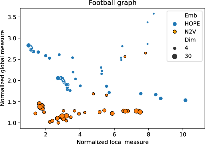
Figure 1. Normalized global and local scores for FOOTBALL graph.
We recommend to select the best embedding by careful investigation of both scores but, alternatively, one can ask the framework to decide which embedding to use in an unsupervised fashion. In order to do it, one may combine the global and the local scores, as explained in Equation (3), to make a decision based on a single combined divergence score. This way we identified the best and the worst embeddings. To visualize the selected embeddings in high dimensions, we needed to perform dimension reduction that seeks to produce a low-dimensional representation of high-dimensional data that preserve relevant structure. For that purpose, we used the Uniform Manifold Approximation and Projection (UMAP)Footnote 9 (McInnes et al., Reference McInnes, Healy and Melville2018), a novel manifold learning technique for dimension reduction. UMAP is constructed from a theoretical framework based in Riemannian geometry and algebraic topology; it provides a practical scalable algorithm that applies to real-world datasets. The results are presented in Figure 2. The embedding presented on the left-hand side shows the winner that seems to not only separate nicely the communities but also puts pairs of communities far from each other if there are few edges between them; as a result, both scores are good. The embedding in the middle separates communities, but the nodes within communities are clumped together resulting in many edges that are too short. There are also a lot of edges that are too long. As a result, the local score for this embedding is bad. Finally, the embedding on the right has a clear problem with distinguishing communities, and some of them are put close to each other resulting in a bad global score.
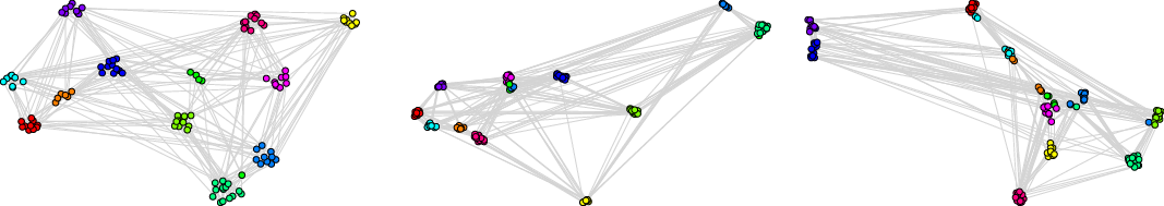
Figure 2. Two-dimensional projections of embeddings of FOOTBALL graph according to the framework: the best (left), the worst with respect to the local score (middle), and the worst with respect to the global score (right).
4.4 Approximating the two scores
Let us start with an experiment testing whether our scalable implementation provides a good approximation of both measures, the density-based (global) score $\Delta _{\mathcal E}^g(G)$
and the link-based (local) score
$\Delta _{\mathcal E}^g(G)$
and the link-based (local) score $\Delta _{\mathcal E}^{\ell }(G)$
. We tested SBM, LFR, and noisy-LFR graphs with the two available embeddings (using the parameters and selected dimensions as described above). The number of landmarks was set to be five times larger than the number of communities in each graph, namely SBM graph used
$\Delta _{\mathcal E}^{\ell }(G)$
. We tested SBM, LFR, and noisy-LFR graphs with the two available embeddings (using the parameters and selected dimensions as described above). The number of landmarks was set to be five times larger than the number of communities in each graph, namely SBM graph used $30\times 5 = 150$
landmarks, LFR had
$30\times 5 = 150$
landmarks, LFR had $75\times 5 = 375$
landmarks, and for noisy-LFR the number of landmarks was set to
$75\times 5 = 375$
landmarks, and for noisy-LFR the number of landmarks was set to $54\times 5 = 270$
.
$54\times 5 = 270$
.
Figures 3 and 4 present the results of experiments for LFR graph and both embedding algorithms. (Experiments for other graphs can be found in the supplementary document.) The first figure shows how well the global score is approximated by a scalable algorithm and the second figure concentrates on the local score. Recall that graphs on $10{,}000$
nodes are, by default, the smallest graphs for which the framework uses scalable algorithm. The default setting in the framework is to use at least
$10{,}000$
nodes are, by default, the smallest graphs for which the framework uses scalable algorithm. The default setting in the framework is to use at least $4$
landmarks per community and at least
$4$
landmarks per community and at least $4\sqrt{n}$
of them overall, so
$4\sqrt{n}$
of them overall, so $400$
landmarks for graphs of size
$400$
landmarks for graphs of size $10{,}000$
and many more for larger graphs. In our experiment, we see good results with even fewer landmarks. This was done in purpose to test approximation precision in a challenging corner case. As expected, global properties reflected by the global score are easier to approximate than local properties investigated by the local score that are more sensitive to small perturbations. Nevertheless, both scores are approximated to a satisfactory degree. The Pearson correlation coefficients for both HOPE and Node2Vec are close to 1 for the global score and roughly 0.99 for the local score. For other standard correlation measures, see Tables 1 and 2.
$10{,}000$
and many more for larger graphs. In our experiment, we see good results with even fewer landmarks. This was done in purpose to test approximation precision in a challenging corner case. As expected, global properties reflected by the global score are easier to approximate than local properties investigated by the local score that are more sensitive to small perturbations. Nevertheless, both scores are approximated to a satisfactory degree. The Pearson correlation coefficients for both HOPE and Node2Vec are close to 1 for the global score and roughly 0.99 for the local score. For other standard correlation measures, see Tables 1 and 2.
Figure 3. Approximated vs. exact global scores for LFR graphs and HOPE (left) and Node2Vec (right) embeddings.
Figure 4. Approximated vs. exact local scores for LFR graphs and HOPE (left) and Node2Vec (right) embeddings.
Table 1. Correlation between approximated and (exact) global scores
Table 2. Correlation between approximated and (exact) local scores
Finally, we checked if the number of landmarks used by the framework as a default value (namely, $4\sqrt{n}$
) is a good choice. We see in Figures 5 and 6 that the approximation quickly stabilizes, and so there is no need for a large number of landmarks to get the desired approximation. As commented earlier, the local score is more challenging to approximate (see Figure 6 again), and the Pearson correlation between the approximated and the exact local scores does not seem to tend to 1 quickly but it is very close to 1, providing a satisfactory precision.
$4\sqrt{n}$
) is a good choice. We see in Figures 5 and 6 that the approximation quickly stabilizes, and so there is no need for a large number of landmarks to get the desired approximation. As commented earlier, the local score is more challenging to approximate (see Figure 6 again), and the Pearson correlation between the approximated and the exact local scores does not seem to tend to 1 quickly but it is very close to 1, providing a satisfactory precision.
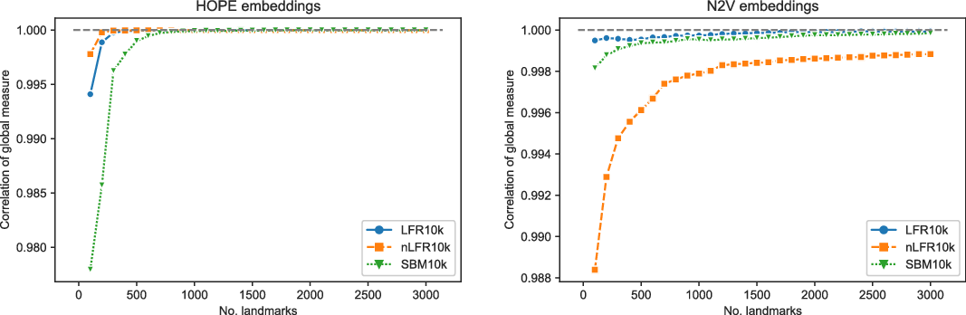
Figure 5. Pearson’s correlation between approximated and exact global scores for SMB, LFR, noisy-LFR graphs, and HOPE (left) and Node2Vec (right) embeddings.

Figure 6. Pearson’s correlation between approximated and exact local scores for SMB, LFR, noisy-LFR graphs, and HOPE (left) and Node2Vec (right) embeddings.
4.5 Node classification and community detection vs. the global score
It is expected and desired that the global score measures how useful a given embedding is for any application that requires a good understanding of a global structure of the network. In our next experiments, we tested two such applications: node classification and community detection.
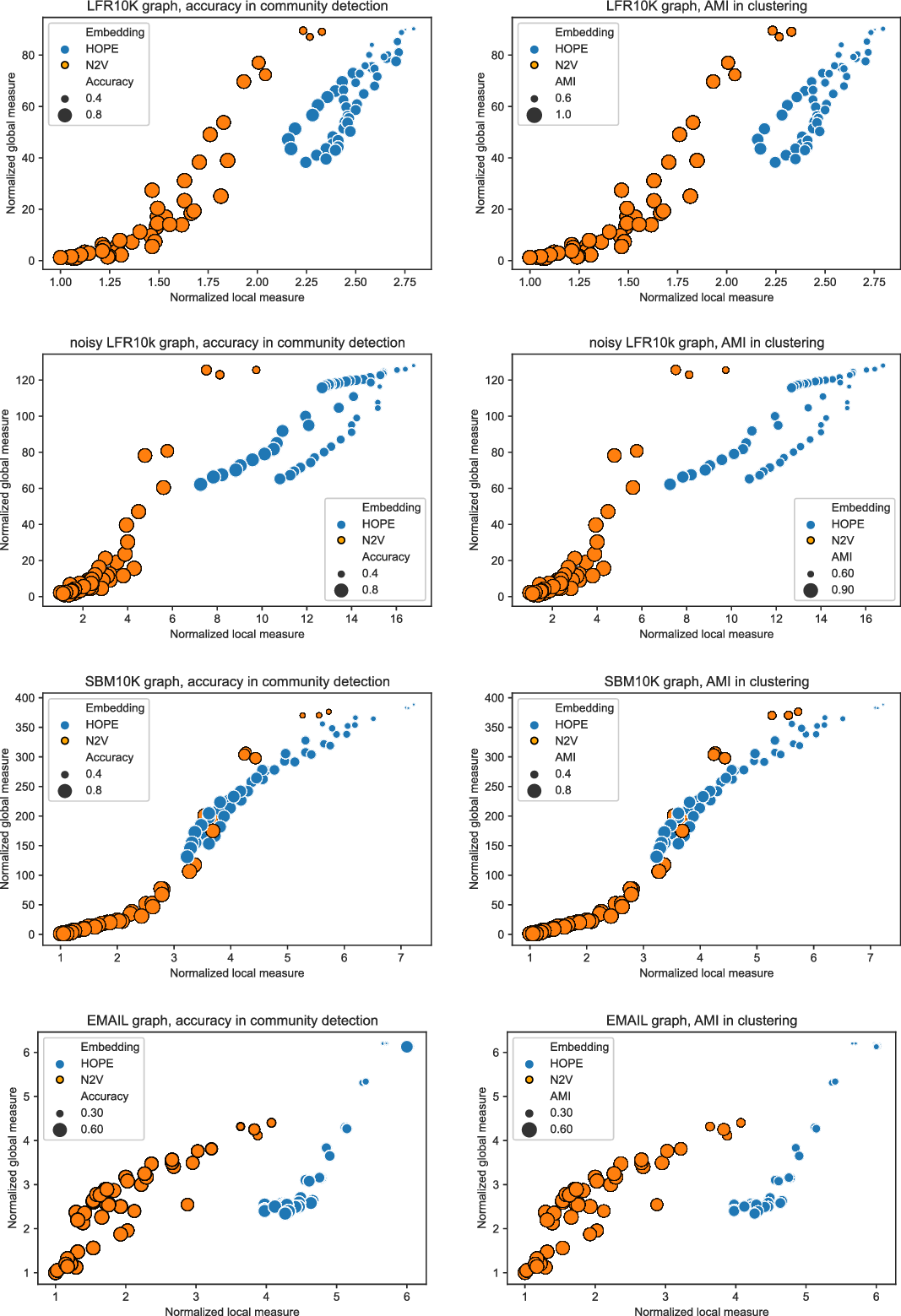
Figure 7. Global and local scores with accuracy (left) and AMI (right) overlay for SBM, LFR, noisy-LFR, EMAIL graphs, and HOPE and Node2Vec embeddings.
Node classification task aims to train a model to learn to which class a node belongs to. Typically, the goal is to label each node with a categorical class (binary classification or multi-class classification) or to predict a continuous number (regression). The process is supervised in nature, that is, the model is trained using a subset of nodes that have ground-truth labels.
For each graph (SBM, LFR, noisy-LFR, and EMAIL), each of the two embeddings (HOPE and Node2Vec) was used as an input for community detection task based on XGBoost model. XGBoostFootnote 10 is an open-source software library that provides a regularizing gradient boosting framework, the algorithm of choice for many winning teams of machine learning competitions. Since we aim to have a fair benchmark evaluating if an embedding extracts any useful global properties of the network instead of optimizing the quality of the outcome, we used vanilla XGBoost with default hyperparameters. For each embedding, we conducted 10 independent repetitions of the standard training process. First, nodes with the corresponding embedding was randomly partitioned into a training and a test set (25% of all observations). Then, XGBoost model was trained on the training set together with the corresponding labels indicated the ground-truth community the nodes belong to. Finally, the model was used to predict the communities on the test set, and the accuracy was reported.
Similarly, in order to investigate how much of the community structure got preserved by the evaluated embeddings, each embedding was independently clustered 20 times using the classic $k$
-means algorithm, a well-known method that aims to partition
$k$
-means algorithm, a well-known method that aims to partition $n$
vectors into
$n$
vectors into $k$
clusters in which each vector belongs to the cluster with the nearest mean (center of mass). As before, since we aim for a fair and easy benchmark rather than a carefully tuned specific approach, we simply used the vanilla
$k$
clusters in which each vector belongs to the cluster with the nearest mean (center of mass). As before, since we aim for a fair and easy benchmark rather than a carefully tuned specific approach, we simply used the vanilla $k$
-means algorithm and the value of
$k$
-means algorithm and the value of $k$
set to the true number of communities. The AMI score was then calculated based on the two partitions of the set of nodes: the clusters assignment returned by the
$k$
set to the true number of communities. The AMI score was then calculated based on the two partitions of the set of nodes: the clusters assignment returned by the $k$
-means algorithm and the ground-truth communities. This approach is similar to the one used in the recent paper (Tandon et al., Reference Tandon, Albeshri, Thayananthan, Alhalabi, Radicchi and Fortunato2021) in which the authors investigate if embeddings can be used to detect communities.
$k$
-means algorithm and the ground-truth communities. This approach is similar to the one used in the recent paper (Tandon et al., Reference Tandon, Albeshri, Thayananthan, Alhalabi, Radicchi and Fortunato2021) in which the authors investigate if embeddings can be used to detect communities.
The results of both experiments are presented on Figure 7 (the accuracy score for node classification task is presented on the left side, whereas the AMI score for community detection task can be found on the right side). The embeddings that are identified by the framework as good (left-bottom corner, close to the auxiliary point $(1,1)$
representing the hypothetical perfect score) tend to perform well in both applications (large balls representing large values of the accuracy/AMI). On the other hand, poorly scored embeddings (top-right corner) perform poorly (small balls). The same conclusion is obtained after more rigorous investigation of the correlation coefficients between the accuracy/AMI and the global/local scores (see Table 3 and, respectively, Table 4). Let us note that the rank-based correlations (Spearman and Kendall-Tau) report a smaller correlation for Node2Vec embeddings as in our experiment we generated many embeddings that were comparable and of very good quality. As a result, their rankings with respect to the global/local scores and the accuracy/AMI might not be exactly the same but, in any case, the framework was able to distinguish good embeddings from bad ones. More experiments can be found in the supplementary document. In particular, since the accuracies and the AMI scores are not always easy to compare on Figure 7, we present them directly as functions of local and global scores.
$(1,1)$
representing the hypothetical perfect score) tend to perform well in both applications (large balls representing large values of the accuracy/AMI). On the other hand, poorly scored embeddings (top-right corner) perform poorly (small balls). The same conclusion is obtained after more rigorous investigation of the correlation coefficients between the accuracy/AMI and the global/local scores (see Table 3 and, respectively, Table 4). Let us note that the rank-based correlations (Spearman and Kendall-Tau) report a smaller correlation for Node2Vec embeddings as in our experiment we generated many embeddings that were comparable and of very good quality. As a result, their rankings with respect to the global/local scores and the accuracy/AMI might not be exactly the same but, in any case, the framework was able to distinguish good embeddings from bad ones. More experiments can be found in the supplementary document. In particular, since the accuracies and the AMI scores are not always easy to compare on Figure 7, we present them directly as functions of local and global scores.
Table 3. Correlation coefficients between the accuracy scores in node classification task and global/local scores (averaged over all parameters)
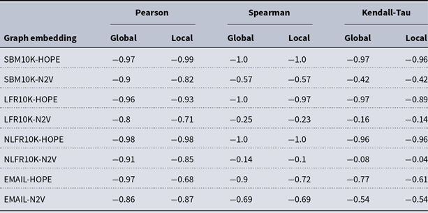
Table 4. Correlation coefficients between the AMI scores in community detection task and global/local scores (averaged over all parameters)

4.6 Link prediction vs. the local score
As discussed in the previous section, the global score returned by the framework captures how well the embedding preserves global properties of embedded networks. Similarly, it is expected and desired that the local score evaluates the power of embeddings to encapsulate local properties. In the next experiment, we tested one local algorithm, namely, link prediction algorithm.
Indeed, most the the methods for directed graph embeddings are validated via link prediction (Zhou et al., Reference Zhou, Liu, Liu, Liu and Gao2017), where one deletes a subset of edges (typically randomly selected) and then measures how well they can be recovered. A commonly used scoring method is the AUC obtained from ranking of node pairs from most to least likely to have an edge between them. A variation of that approach is known as node recommendation, where one removes some outgoing edges for a subset of nodes and try to recover the most likely missing neighbors. Another score that may potentially be used is to compare precision and recall among the top- $k$
candidate node pairs for a specific
$k$
candidate node pairs for a specific $k$
. This is useful, for example, if one has a limited “budget” to investigate if a given pair of nodes are actually linked by an edge or not, so one can only test a small number of pairs.
$k$
. This is useful, for example, if one has a limited “budget” to investigate if a given pair of nodes are actually linked by an edge or not, so one can only test a small number of pairs.
In our experiments, for each of the four graphs we tested (SBM, LFR, noisy-LFR, and EMAIL), given graph $G$
, we randomly selected 5% of its edges and removed them to form a graph
$G$
, we randomly selected 5% of its edges and removed them to form a graph $G'$
. Then we took another random sample of nonadjacent pairs of nodes in
$G'$
. Then we took another random sample of nonadjacent pairs of nodes in $G$
, set
$G$
, set $E'$
. Both classes had the same number of pairs of nodes so that the test set created in such a way was balanced. Our goal was to train a model that uses one of the embeddings of graph
$E'$
. Both classes had the same number of pairs of nodes so that the test set created in such a way was balanced. Our goal was to train a model that uses one of the embeddings of graph $G'$
to detect which pairs of nodes in
$G'$
to detect which pairs of nodes in $E \cup E'$
are adjacent in
$E \cup E'$
are adjacent in $G$
. We repeated this process independently five times (with five different seed values) and reported the average AUC scores.
$G$
. We repeated this process independently five times (with five different seed values) and reported the average AUC scores.
For each of the two algorithms (HOPE and Node2Vec), each combination of their parameters and 16 dimensions we tested, we produced an embedding of graph $G'$
. For evaluation purpose, we computed both the global and the local divergence scores for the produced embedding. In order to create a training set for the classifier, we considered all pairs of adjacent nodes in
$G'$
. For evaluation purpose, we computed both the global and the local divergence scores for the produced embedding. In order to create a training set for the classifier, we considered all pairs of adjacent nodes in $G'$
(the positive class) as well as a random subset of pairs of nonadjacent nodes (the negative class) that is of the same size as the number of edges in
$G'$
(the positive class) as well as a random subset of pairs of nonadjacent nodes (the negative class) that is of the same size as the number of edges in $G'$
(as for the test sets, to keep both classes balanced). Finally, we concatenated embeddings of pairs of nodes representing edges/non-edges into feature vectors to be used for prediction. Such training set was used to train XGBoost model with default hyperparameter values. As already mentioned, in order to measure the quality of this simple model, we computed the AUC score that provides a measure of separability, as it tells us how capable the model is of distinguishing between the two classes, edges
$G'$
(as for the test sets, to keep both classes balanced). Finally, we concatenated embeddings of pairs of nodes representing edges/non-edges into feature vectors to be used for prediction. Such training set was used to train XGBoost model with default hyperparameter values. As already mentioned, in order to measure the quality of this simple model, we computed the AUC score that provides a measure of separability, as it tells us how capable the model is of distinguishing between the two classes, edges $E$
and non-edges
$E$
and non-edges $E'$
, both coming from the original graph
$E'$
, both coming from the original graph $G$
. (Note that some pairs of nodes in the test set might overlap with pairs of nodes in the training set. Even more, some positive pair in the test set might be negative in the training one.)
$G$
. (Note that some pairs of nodes in the test set might overlap with pairs of nodes in the training set. Even more, some positive pair in the test set might be negative in the training one.)
The results of this experiment are presented on Figure 8. The embeddings that score well by the framework (left-bottom corner of the plots, near to the auxiliary point $(1,1)$
) turn out to perform well in predicting links (large balls representing large values of AUC), and the opposite is true for the embeddings that are identified as poor ones (right-top corner of the plots). More rigorous approach can be found in Table 5 where the correlation coefficients between the AUC and the global/local scores are reported. As before, since there are many Node2Vec embeddings that are almost indistinguishable, ranking-based correlation coefficients report weaker correlation. The framework has no chance to predict the exact ranking of the embeddings based on their global/local scores, but it is clearly able to identify good embeddings and separate them from bad ones. As usual, more experiments can be found in the supplementary document, including counterpart of Figure 8 presenting the AUC score as functions of local and global scores.
$(1,1)$
) turn out to perform well in predicting links (large balls representing large values of AUC), and the opposite is true for the embeddings that are identified as poor ones (right-top corner of the plots). More rigorous approach can be found in Table 5 where the correlation coefficients between the AUC and the global/local scores are reported. As before, since there are many Node2Vec embeddings that are almost indistinguishable, ranking-based correlation coefficients report weaker correlation. The framework has no chance to predict the exact ranking of the embeddings based on their global/local scores, but it is clearly able to identify good embeddings and separate them from bad ones. As usual, more experiments can be found in the supplementary document, including counterpart of Figure 8 presenting the AUC score as functions of local and global scores.
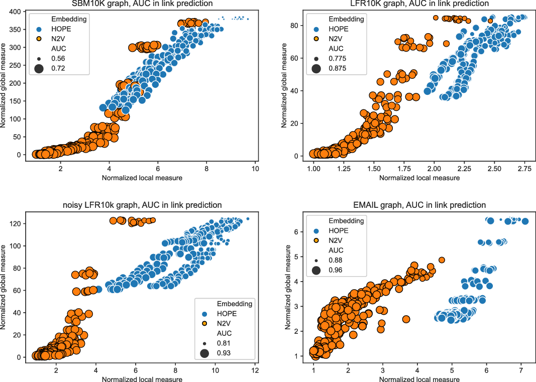
Figure 8. Global and local scores with AUC overlay for SBM, LFR, noisy-LFR, EMAIL graphs, and HOPE and Node2Vec embeddings.
4.7 More challenging situations
Based on experiments in Section 4.5, we see that both global (as expected) and local (far from being obvious) scores correlate well with the quality of both node classification and community detection. Similarly, experiments in Section 4.6 imply that both scores correlate with the quality of link prediction algorithm (this time, we expect this from the local score but not necessarily from the global one). We see such behavior as the two scores often correlate with one another. Indeed, for a relatively easy graph to deal with, a good quality embedding should be able to preserve both local and global properties of the network. On the other hand, poor quality embeddings (e.g., when the dimension is too small or the parameters are not properly selected) typically fail to produce anything useful, from any of the two perspectives. Our synthetic models and EMAIL graph seem to confirm this. However, it is expected and plausible that large, real-world graphs are more challenging to deal with. For such graphs, it might be difficult if not impossible to find an embedding that scores well from both perspectives. In such situations, one needs to make a decision which embedding to use based on a specific application at hand (using either global or local properties). In order to illustrate such situations, we experimented with an undirected ABCD graph and $32$
-dimensional Node2Vec embedding (with parameters set to
$32$
-dimensional Node2Vec embedding (with parameters set to $p=q=1$
).
$p=q=1$
).
First, we rewired a specified fraction $p$
of edges within each community. The rationale behind it is that such operation should destroy local properties of the embedding (many edges within communities are now long with respect to the associated embedding and some pairs of close nodes are not adjacent), but global properties should remain unchanged.
$p$
of edges within each community. The rationale behind it is that such operation should destroy local properties of the embedding (many edges within communities are now long with respect to the associated embedding and some pairs of close nodes are not adjacent), but global properties should remain unchanged.
We independently generated five graphs with the following rewiring fractions: $p=0.2$
,
$p=0.2$
, $p=0.4$
,
$p=0.4$
, $p=0.6$
,
$p=0.6$
, $p=0.8$
, and
$p=0.8$
, and $p=1.0$
; note that
$p=1.0$
; note that $p=0$
corresponds to the original ABCD graph. As expected, the global score and the quality of both node classification and community detection algorithms remain the same. More importantly, the local score increases (the quality of the embedding gets worse) and the quality of link prediction algorithm (AUC) gets worse—see Figure 9 (left).
$p=0$
corresponds to the original ABCD graph. As expected, the global score and the quality of both node classification and community detection algorithms remain the same. More importantly, the local score increases (the quality of the embedding gets worse) and the quality of link prediction algorithm (AUC) gets worse—see Figure 9 (left).
Table 5. Correlation coefficients between the AUC scores in link prediction task and global/local scores (averaged over all parameters)
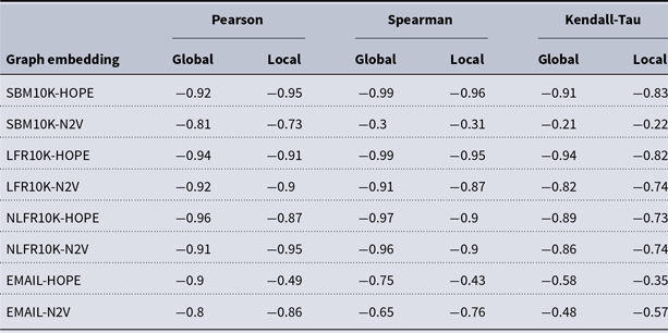
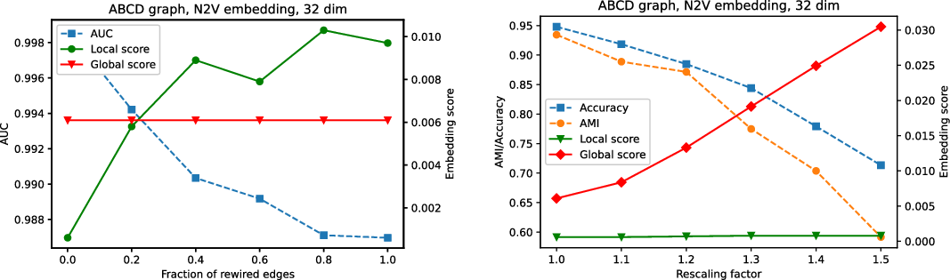
Figure 9. Comparison of local/global scores (and associated quality measures for various tasks) for rewired graphs (left) and rescaled embeddings (right).
In order to test the opposite scenario, we kept the original ABCD graph but slightly modified the original embedding. Each community was independently rescaled by a factor of $q\gt 1$
. Formally, all points in the embedding that are associated with nodes that belong to a given community increased their distance from the center of mass of this community while keeping the direction from it. The idea behind this approach is that, on average, the distance between nodes from different communities (most pairs of nodes) remain the same, and the distance between nodes within one community is only slightly increased (small fraction of pairs of nodes anyway). As a result, local properties should be preserved almost as well as in the original embedding. On the other hand, inflated communities tend to overlap more in the embedded space than before and, as a result, the global quality measure should decrease.
$q\gt 1$
. Formally, all points in the embedding that are associated with nodes that belong to a given community increased their distance from the center of mass of this community while keeping the direction from it. The idea behind this approach is that, on average, the distance between nodes from different communities (most pairs of nodes) remain the same, and the distance between nodes within one community is only slightly increased (small fraction of pairs of nodes anyway). As a result, local properties should be preserved almost as well as in the original embedding. On the other hand, inflated communities tend to overlap more in the embedded space than before and, as a result, the global quality measure should decrease.
We independently generated five embeddings with the following rescaling factors: $q=1.1$
,
$q=1.1$
, $q=1.2$
,
$q=1.2$
, $q=1.3$
,
$q=1.3$
, $q=1.4$
, and
$q=1.4$
, and $q=1.5$
; note that
$q=1.5$
; note that $q=1$
corresponds to the original embedding. As expected, the local score and the quality of link prediction algorithm remain the same. More importantly, the global score increases (the quality of the embedding gets worse), and the quality of both node classification (accuracy) and community detection (AMI) get worse—see Figure 9 (right).
$q=1$
corresponds to the original embedding. As expected, the local score and the quality of link prediction algorithm remain the same. More importantly, the global score increases (the quality of the embedding gets worse), and the quality of both node classification (accuracy) and community detection (AMI) get worse—see Figure 9 (right).
The conclusion can be summarized as follows. Global score might not be able to detect problems with a given embedding if these problems are local by nature. For example, despite the fact that an embedding properly captures between-community distances, it may inaccurately reflect relationships between nodes within communities. On the other hand, local score might fail to capture the fact that in the embedding, communities (treated globally as a cloud of points) are not appropriately separated. For this reason, although in many cases global and local scores are consistent, they are in general not equivalent and it is useful to calculate them both and investigate carefully.
5. Conclusions
In this paper, we introduced a framework that assigns two scores (global and local) for embeddings of a given graph. The two scores measure the ability of analyzed embeddings to preserve global and, respectively, local properties of the embedded graph. The code is written in Julia (high-level, high-performance, and dynamic programming language) and available onlineFootnote 11. The framework is easy to use (knowledge of Julia is not required to use it; default parameters should be suitable for most cases) and flexible (more advanced users may modify parameters, if needed).
If the embeddings need to be used for unsupervised tasks, the framework is able to identify the best embedding in an unsupervised way via combined divergence score. However, the user might still want to consider a few embeddings that score well from both perspectives and, if possible, select an embedding generated by a simple/explainable algorithm. In particular, there is usually no need to use very high-dimensional embeddings if the improvement is marginal. On the other hand, if the embedding is to be used for supervised tasks, the best course of action might be to consider a number of top-scoring embeddings and select the winner by performing a standard supervised selection for a given application at hand.
Let us also discuss some potential future directions. In Dehghan-Kooshkghazi et al. (Reference Dehghan-Kooshkghazi, Kamiński, Kraiński, Prałat and Théberge2020), some throughout analysis of the original framework for undirected graphs (and using only the global score) was performed. A natural next step is to test in more detail the current version of the framework (using the two scores) on both real-world and synthetic networks. More importantly, it would be valuable to show the predictive power and usefulness of the framework for a large dataset and some real-world important application. The industry partners we collaborate with provide a positive feedback so far, but having a publishable results of experiments performed on publicly available datasets will be of high value.
When analyzing the correlation between the link prediction algorithm and the local score (Section 4.6), we independently performed a few more experiments investigating the reason why embeddings are able to predict missing links. In particular, we created two additional training sets. The first training set was the same as the original one but with five additional columns: in-degree and out-degree for both nodes as well as the distance between them. The second training set consisted with only these five additional columns. The quality of models obtained by using both such training sets turned out to be comparable to the original one we used for our tests. As expected, the richer set typically gave slightly better quality results but not always. This implies that the embeddings encoded the most important information about the graph via the distances between nodes (or XGBoost was not able to extract more from other sources). This suggests that the GCL model should be able to accurately model the shape of the embedded networks as they require exactly the five columns as the parameters/input. We plan to use the GCL model, along with graph-based communities and other properties such as transitive closure, to build a better quality link prediction algorithm. Another potential and important application is to detect overlapping communities or to detect anomalies. In both cases, the GCL model equipped with a good embedding would be the heart of such an algorithm.
Competing interests
None.
Supplementary materials
For supplementary material for this article, please visit http://doi.org/10.1017/nws.2022.27


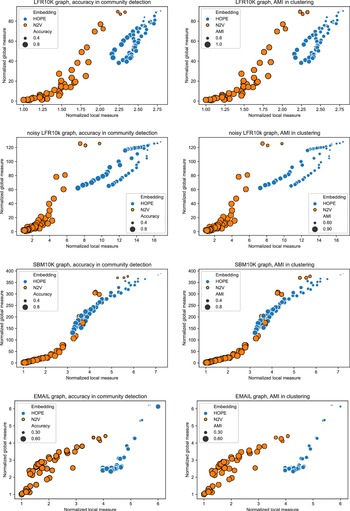


 Open access