


1. Introduction
Magnetoconvection (MC) governs most astro- and geophysical systems and is relevant to various engineering applications (Weiss & Proctor Reference Weiss and Proctor2014; Davidson Reference Davidson2016). The former include, for instance, outer layers of stars and liquid-metal planetary cores (Jones Reference Jones2011), examples of the latter comprise liquid-metal batteries, electromagnetic brakes in continuous casting, liquid-metal cooling for nuclear fusion reactors and semiconductor crystal growth (Davidson Reference Davidson1999). Magnetoconvection occurs in an electrically conducting fluid that is subjected to both a magnetic field and an imposed temperature gradient. The buoyancy forces induce convective fluid motion due to thermal expansion and contraction, while the magnetic field affects this motion and distorts the global flow structure through the Lorentz force, which eventually influences the heat transport in the system. The resulting main two control parameters, the strength of the imposed thermal driving and that of the external magnetic field, are encoded in independent dimensionless groups, the Rayleigh number  $Ra$ and Hartmann number $Ha$, respectively, while the ratio of viscous to thermal diffusion coefficients, the Prandtl number, defines the working fluid:
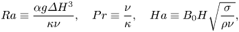 \begin{equation} Ra\equiv \frac{\alpha g \varDelta H^3}{\kappa \nu},\quad Pr\equiv \frac{\nu}{\kappa},\quad Ha\equiv B_0 H \sqrt{\frac{\sigma}{\rho \nu}}, \end{equation}
where  $\sigma$ is the electrical conductivity, $\rho$ the mass density, $\alpha$ the thermal expansion coefficient, $g$ the acceleration due to gravity, $\nu$ the kinematic viscosity, $\kappa$ the thermal diffusivity, $\varDelta$ the temperature difference between bottom and top plate, $B_0$ the external magnetic field strength, and $H$ the domain height.
One of the key objectives in MC research is to provide scaling relations for the heat transport through the system, represented in dimensionless form by the ratio of total to conductive heat flux, the Nusselt number  $Nu$, as a function of $Ra$ and $Ha$. However, the heat transport scaling relations also depend on the flow configuration, including the angle between the magnetic field and gravity, the geometry of the container and the boundary conditions (BCs), and on whether the buoyancy forces dominate over the Lorentz forces in the system or vice versa. This inherent complexity results in the need, at least in principle, to derive separate heat transport scaling relations to describe each specific flow regime itself and transitions between distinct regimes. The considerable difficulty of doing so in a coherent manner is exacerbated by non-universal scaling relations even within specific regimes – the scaling relations in the buoyancy-dominated and Lorentz-force-dominated regimes themselves change with the control parameters, and transitions between the different regimes are also non-universal.
The objective of this paper is to offer a unifying heat transport model for the transition between the buoyancy-dominated and Lorentz-force-dominated regimes in quasistatic MC. We focus on Rayleigh–Bénard convection (RBC) (Ahlers, Grossmann & Lohse Reference Ahlers, Grossmann and Lohse2009) with an applied vertical magnetic field and assume that the magnetic field is constant in the entire domain, without being affected by a fluid motion or finite magnetic diffusion. The model uses the theoretical predictions by Grossmann and Lohse (Grossmann & Lohse Reference Grossmann and Lohse2000, Reference Grossmann and Lohse2001; Stevens et al. Reference Stevens, van der Poel, Grossmann and Lohse2013) for RBC without magnetic field and transfers the approach by Ecke and Shishkina (Ecke & Shishkina Reference Ecke and Shishkina2023, § 3.3) for transitions in rotating RBC to the case of RBC with a vertical magnetic field. To verify the proposed model, we compare the theoretical predictions with results for liquid-metal MC obtained by direct numerical simulation (DNS) carried out by us and others (Liu, Krasnov & Schumacher Reference Liu, Krasnov and Schumacher2018; Yan et al. Reference Yan, Calkins, Maffei, Julien, Tobias and Marti2019; Akhmedagaev et al. Reference Akhmedagaev, Zikanov, Krasnov and Schumacher2020; Xu, Horn & Aurnou Reference Xu, Horn and Aurnou2023), as well as experiments (Cioni, Chaumat & Sommeria Reference Cioni, Chaumat and Sommeria2000; King & Aurnou Reference King and Aurnou2015; Zürner et al. Reference Zürner, Schindler, Vogt, Eckert and Schumacher2020; Xu et al. Reference Xu, Horn and Aurnou2023). In addition, we carried out simulations for a different working fluid at higher Prandtl number  $Pr$ to compare our DNS data with that from Lim et al. (Reference Lim, Chong, Ding and Xia2019). The predictions of the proposed model agree well with the experimental and DNS data.
2. Model for regime transition
We consider a layer of electrically conducting fluid confined between two infinitely wide and long plates, driven by a buoyancy force generated by an imposed vertical temperature difference between the top and bottom plates, and subjected to a uniform vertically orientated magnetic field. We further consider the flow to be turbulent, that is, in a regime sufficiently far from bulk onset such that the heat transport obeys a power-law dependence on the thermal driving. When the magnetic field is weak compared with the buoyancy force, we recover classical RBC scaling for the dimensionless convective heat flux  $Nu-1$, that is, the total dimensionless heat flux $Nu$ less its conductive contribution, $Nu - 1 \sim (Ra/Ra_{c,b})^\gamma \sim Ra^\gamma$, for an exponent $\gamma$, where $Ra_{c,b}$ is the critical $Ra$ for RBC bulk onset for a given container geometry. When the Lorentz force is strong compared with the buoyancy force, we expect a similar scaling law $Nu - 1 \sim (Ra/Ra_{c,L})^\xi$, for an exponent $\xi$. Here, the dependence on the critical Rayleigh number $Ra_{c,L}$ in the Lorentz-force-dominated regime is kept due to its dependence on $Ha$, which can be obtained from linear stability theory (Chandrasekhar Reference Chandrasekhar1961) $Ra_{c,L} \sim Ha^2$, with no dependence on the Prandtl number.
Although these buoyancy-dominated and Lorentz-force-dominated scaling laws appear disconnected, they are intrinsically linked under the assumption that they must overlap at some intermediate region between the two extreme regimes, where the influence of neither the Lorentz force or buoyancy force on the convective heat transport can be ignored. In order to derive a model connecting the two scaling laws, we make two key assumptions; (i) the thermal and Hartmann boundary layers (BLs) scale as  $\delta _T \propto 1/Nu$ and $\delta _\nu \propto 1/Ha$, respectively, and (ii) there is a transition point at a universal ratio of BL thicknesses across parameter space. The former are the well-known classical scaling relations for laminar BLs, and there is ample experimental and numerical evidence for the relations to hold. We will revisit this point in § 4.1. For the latter, we postulate that at the transition between these regimes, the two corresponding scaling laws will cross over,
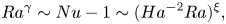 \begin{equation} Ra^\gamma\sim Nu-1\sim(Ha^{-2}Ra)^\xi, \end{equation}
and, to construct a relationship between the two scaling exponents  $\gamma$ and $\xi$, we assume that this cross-over occurs at a $Pr$-dependent ratio of the thermal and viscous boundary layer thicknesses that is independent of the control parameters $Ra$ and $Ha$. For $Pr > 1$, this ratio may be close to unity as the thermal BL is nested within the viscous or Hartmann layer at moderate value of $Ha$. Increasing $Ha$ results in a thinner Hartmann layer and thus eventually to a BL crossing. However, for $Pr \ll 1$, as is the case for liquid metals, the Hartmann layer is much thinner than the thermal BL. Hence depending on the strength of the external magnetic field, very strong thermal driving is required to quench the thermal BL to become thinner than the Hartmann layer, and a BL cross-over will only occur far in the buoyancy-dominated regime, if at all (Zürner Reference Zürner2020). We will return to this point in § 4.1.
Assuming  $\delta _T = \beta \delta _{\nu }$ for a constant $\beta = \beta (Pr)$ at the transition implies $Nu \sim Ha$. Since this transition is seen to typically occur at high Nusselt numbers, meaning $Nu \approx Nu-1$, we obtain
 \begin{equation} Ha \sim Nu \sim Ra^\gamma \sim Ra^\xi Ha^{-2\xi} \sim Ra^{-2\xi\gamma+\xi}, \end{equation}
resulting in the following relationship between the exponents:
 \begin{equation} \xi={\gamma/(1-2\gamma)},\quad \textrm{or}\quad \gamma={\xi/(1+2\xi)}. \end{equation}
One can see that a larger (smaller) exponent in one regime requires a larger (smaller) exponent in the other regime, and that  $\gamma$ is always smaller than $1/2$. The latter suggests that the ultimate regime can be attained only asymptotically, under overwhelming dominance of buoyancy over Lorentz force, and may not be attained under the dominance of magnetic fields, as the Lorentz force suppresses turbulence.
In figure 1 we present a sketch of the proposed scaling relations for  $(Nu-1)$ vs $Ha$ (figure 1a) and $Ra$ (figure 1b), according to the relations (2.3). Once $\gamma$ is known for any specific $Pr$, the exponent $\xi$ can be calculated from (2.3). These scalings can then be used to define coordinates $(Nu-1)Ra^{-\gamma }$ and $Ha^{-1/\gamma }Ra$ with respect to which the heat transport dependence for different values of $Ha$ and $Ra$ collapse onto a master curve, as sketched in figure 2. The transition then should take place in a Rayleigh-number range that scales as $Ha^{1/\gamma }$.
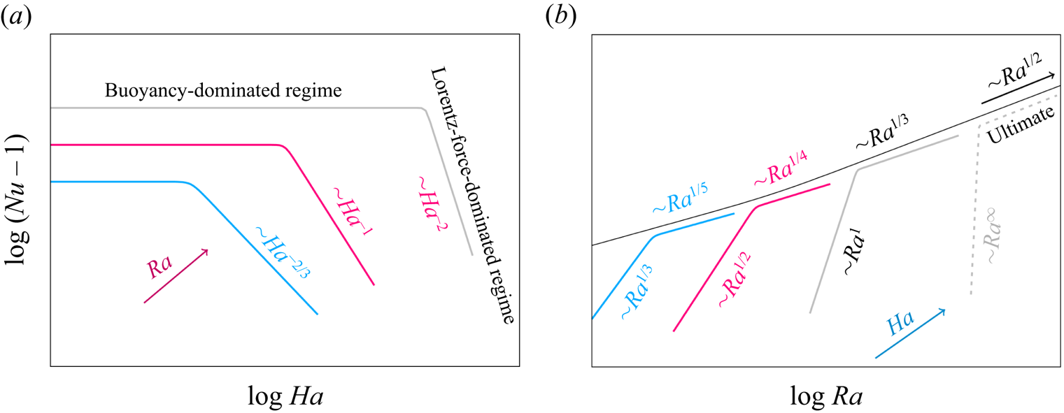
Figure 1. Scalings of  $Nu-1$ vs (a) $Ha$ and (b) $Ra$, according to the theory. The scaling laws $Ha^{-2/3}$ and $Ha^{-1}$ in (a) correspond to $Ra^{1/5}$ and $Ra^{1/4}$ in (b), respectively. These are regimes I and II in the classification provided by GL theory, where $Ra^{1/4}$ refers to the small- $Ra$ regime I, with most of the thermal and kinetic energy dissipation occurring in the BLs. The law $Ra^{1/5}$ (regime II) is predicted to occur at small $Pr$.
$Pr$.
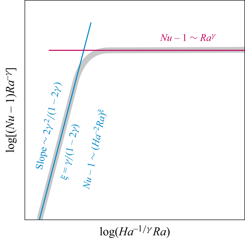
Figure 2. Schematic representation of the normalised convective heat transport  $Nu-1$ displaying the transition from the Lorentz-force-dominated regime, $Nu-1\sim (Ha^{-2}Ra)^\xi$, to the buoyancy-dominated regime, $Nu-1\sim Ra^\gamma$, according to our model. The scaling exponents $\xi$ and $\gamma$ follow (2.3), while the transition scales with $Ha^{-1/\gamma }Ra$.
To close the model, a theoretical prediction for either  $\gamma$ or $\xi$ must be made. The former is readily available through Grossmann–Lohse (GL) theory (Grossmann & Lohse Reference Grossmann and Lohse2000, Reference Grossmann and Lohse2001; Stevens et al. Reference Stevens, van der Poel, Grossmann and Lohse2013) for RBC without magnetic field, applicable here in the buoyancy-dominated regime. An extension of GL theory to MC at finite magnetic Reynolds number was suggested by Chakraborty (Reference Chakraborty2008), Zürner et al. (Reference Zürner, Liu, Krasnov and Schumacher2016) and Zürner (Reference Zürner2020). As the quasistatic approximation applies in the limit of vanishing magnetic Reynolds number, and as we apply GL theory in the buoyancy-dominated regime where the effect of the Lorentz force is weak compared with buoyancy, we do not consider MC-extended GL theory here. Furthermore, for low $Pr$, so far the MC extension describes only the heat transport to a good approximation; effects on momentum transport such as turbulence suppression by a magnetic field appear not to be captured well (Zürner Reference Zürner2020). For any given $Pr$ and $Ra$ range, the theory provides accurate predictions of the value of $\gamma$, for containers of aspect ratio $\varGamma \gtrsim 1$. For $\varGamma \ll 1$, the data can be rescaled according to the method suggested in (Shishkina Reference Shishkina2021; Ahlers et al. Reference Ahlers2022), which we do not discuss here, as in the present study $\varGamma =1$.
3. Experimental and numerical data
To verify the theoretical model, we compare its predictions against data obtained from experiments of liquid-metal MC (Cioni et al. Reference Cioni, Chaumat and Sommeria2000; King & Aurnou Reference King and Aurnou2015; Zürner et al. Reference Zürner, Schindler, Vogt, Eckert and Schumacher2020; Xu et al. Reference Xu, Horn and Aurnou2023) and DNS conducted by us and others (Liu et al. Reference Liu, Krasnov and Schumacher2018; Yan et al. Reference Yan, Calkins, Maffei, Julien, Tobias and Marti2019; Akhmedagaev et al. Reference Akhmedagaev, Zikanov, Krasnov and Schumacher2020; McCormack et al. Reference McCormack, Teimurazov, Shishkina and Linkmann2023; Xu et al. Reference Xu, Horn and Aurnou2023). However, before doing so we provide a brief overview of the data collated from the literature and produced by us to demonstrate the considerable challenges that arise when trying to draw firm conclusions on the scaling of the heat transport with  $Ha$ and $Ra$.
$Ra$.
3.1. Numerical simulations
We simulate an incompressible, viscous buoyancy-driven flow of an electrically conducting fluid in the presence of a static external magnetic field for very small magnetic Reynolds number  $Rm \ll 1$ and magnetic Prandtl number $Pm \ll 1$ by solving numerically the MC equations within the Oberbeck–Boussinesq and quasistatic approximations:
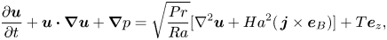 $$\begin{gather} \frac{\partial \boldsymbol{u}}{\partial t} + \boldsymbol{u}\boldsymbol{\cdot} \boldsymbol{\nabla} \boldsymbol{u} + \boldsymbol{\nabla}p =\sqrt{\frac{Pr}{Ra}} [{\nabla}^2 \boldsymbol{u} + Ha^2(\kern 1.5pt\boldsymbol{j} \times \boldsymbol{e}_B)] + T \boldsymbol{e}_z, \end{gather}$$
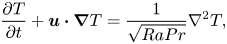 $$\begin{gather}\frac{\partial T}{\partial t} + \boldsymbol{u}\boldsymbol{\cdot}\boldsymbol{\nabla} T = \frac{1}{\sqrt{Ra Pr}} {\nabla}^2 T, \end{gather}$$
 $$\begin{gather}\boldsymbol{\nabla}\boldsymbol{\cdot}\boldsymbol{u} = 0, \end{gather}$$
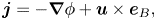 $$\begin{gather}\boldsymbol{j} =-\boldsymbol{\nabla} \phi + \boldsymbol{u} \times \boldsymbol{e}_B, \end{gather}$$
 $$\begin{gather}{\nabla}^2 \phi = \boldsymbol{\nabla}\boldsymbol{\cdot} (\boldsymbol{u} \times \boldsymbol{e}_B) , \end{gather}$$
where  $\boldsymbol {u}$ is the velocity, $T$ the temperature, $p$ the kinematic pressure, $\boldsymbol {j}$ the electric current density, $\phi$ the electric potential, and $\boldsymbol {e}_z$ and $\boldsymbol {e}_B$ are unit vectors that point, respectively, upward (opposite to gravity) and in the direction of the magnetic field $\boldsymbol {B} = B_0 \boldsymbol {e}_B$. The magnetic field is aligned with the buoyancy force, $\boldsymbol {e}_B=\boldsymbol {e}_z$. As for the non-conducting case in the Oberbeck–Boussinesq approximation,
 \begin{equation} Nu = \frac{\langle u_z T\rangle_z - \kappa \partial_z \langle T \rangle_z}{\kappa \varDelta /H}, \end{equation}
where  $\langle {\cdot } \rangle _z$ denotes the time average taken over cross-sections at height $z$.
$z$.
Equations (3.1)–(3.5) have been non-dimensionalised using the container height  $H$, the free-fall velocity $u_{f\!f}\equiv (\alpha gH\varDelta )^{1/2}$, the free-fall time $t_{f\!f}\equiv H/u_{f\!f}$, the temperature difference between the bottom and top plates, $\varDelta \equiv T_+-T_-$, and the external magnetic field strength, $B_0$, as units of length, velocity, time, temperature and magnetic field strength, respectively. We apply no-slip BCs for the velocity at all boundaries, $\boldsymbol {u}=0$, constant temperatures at the end faces, i.e. $T=T_+$ at the bottom plate at $z=0$ and $T=T_-$ at the top plate at $z=H$, and adiabatic BC at the sidewalls, $\partial T/\partial \boldsymbol {n}=0$, where $\boldsymbol {n}$ is the vector orthogonal to the surface. All solid boundaries are considered electrically insulated; Neumann BCs for the electric potential are $\partial \phi /\partial \boldsymbol {n}=0$. The simulation domain is cubic of height $H$, width $W$, length $L$,
$L$,  $H=W=L$, i.e. has aspect ratio $\varGamma \equiv L/H = 1$. Most simulations are carried out for liquid metals such as Ga-In-Sn eutectic alloy at $Pr=0.025$, for $Ra$ up to $10^9$ and $Ha$ up to $2000$. Some DNS are conducted also for $Pr=8$, to extend the parameter range studied in Lim et al. (Reference Lim, Chong, Ding and Xia2019).
Our DNS have been carried out with an MC extension of the direct numerical solver goldfish (Kooij et al. Reference Kooij, Botchev, Frederix, Geurts, Horn, Lohse, van der Poel, Shishkina, Stevens and Verzicco2018; Reiter et al. Reference Reiter, Shishkina, Lohse and Krug2021; Reiter, Zhang & Shishkina Reference Reiter, Zhang and Shishkina2022; McCormack et al. Reference McCormack, Teimurazov, Shishkina and Linkmann2023), which has been widely used in previous studies of different convective flows. The new version of the code that applies a fourth-order finite-volume discretisation on staggered grids and a third-order Runge–Kutta time marching scheme (Reiter et al. Reference Reiter, Shishkina, Lohse and Krug2021, Reference Reiter, Zhang and Shishkina2022) has been extended to simulate magnetoconvective flows, where a consistent and conservative scheme (Ni & Li Reference Ni and Li2012) is utilised to calculate the current density and the Lorentz force. The DNS dataset comprises 38 simulations to cover the necessary ranges in  $Ha$ and $Ra$. To obtain a dataset this large within the available resources, a compromise had to be made in terms of the bulk resolution. Staggered grids are used to provide fine resolution in the core part of the domain and near the rigid walls (Shishkina et al. Reference Shishkina, Stevens, Grossmann and Lohse2010). In the bulk, spatial flow fluctuations are resolved down to 2–5, occasionally 10 Kolmogorov microscales; near the rigid walls we resolve the thermal and Hartmann BLs. To ensure accurate predictions of mean $Nu$, grid refinement studies have been done for key simulations. For these cases, changing the grid resolution by a factor of at least 2.5 resulted in changes of
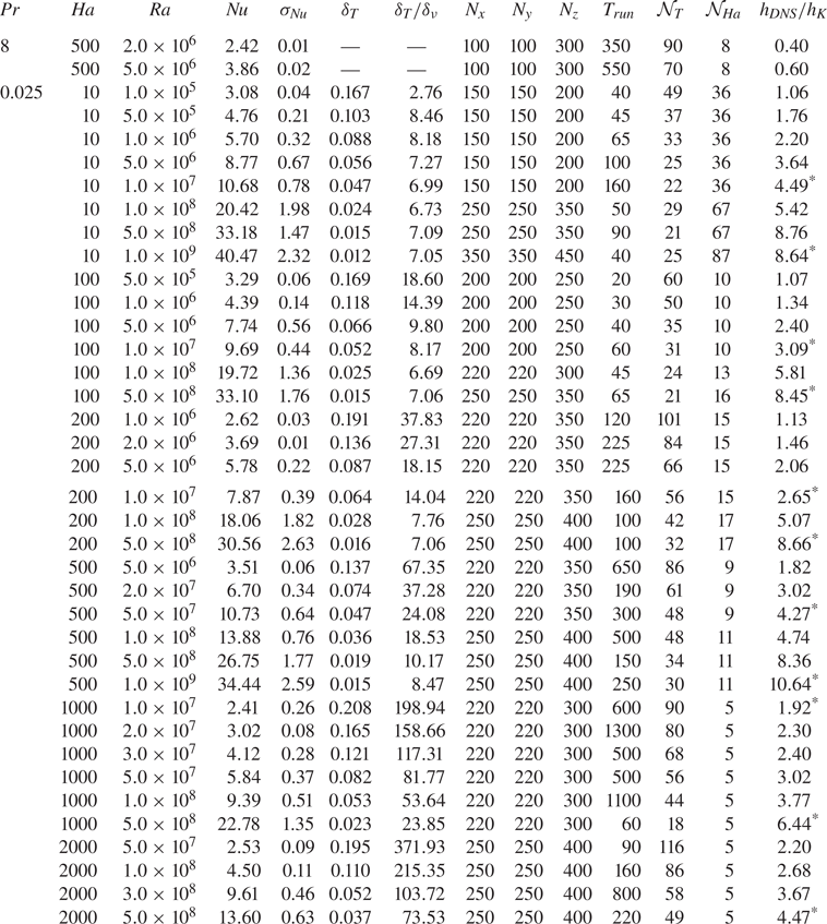
  $Nu$ by less than 1 % over a long-time average. The main parameters of the simulations and key observables are summarised in Appendix A, table 1.
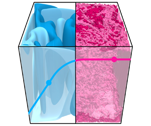
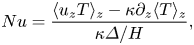
Figure 3 presents example visualisations of the velocity magnitude and temperature, respectively, at an instant in time during statistically steady evolution in the magnetically dominated and the buoyancy-dominated regimes. Panels (a,c) correspond to  $Ra = 10^7$, $Ha = 1000$, (b,d) to $Ra = 10^9$, $Ha = 10$. As can be seen from a comparison of the flow fields between both regimes, both velocity and temperature fluctuate on much smaller scales in the buoyancy-dominated regime. The magnetically dominated regime shows strong vertical flows near the walls, and we note the absence of plumes in the temperature field.
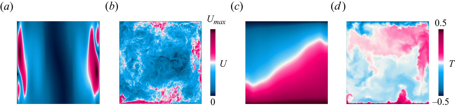
Figure 3. Instantaneous velocity magnitude  $U$ and temperature field $T$ on the $y$ mid-plane for (a,c) $Ra = 10^7$, $Ha = 1000$ and (b,d) $Ra = 10^9$, $Ha = 10$, with $U_{max} = 0.12$ (a) and $U_{max} = 0.8$ (b).
3.2. Summary and comparison of experimental and numerical data
In figure 4 we present  $Nu-1$ as a function of $Ra$ (figure 4a,b) and $Ha$ (figure 4c,d), respectively, from our DNS, experimental (Cioni et al. Reference Cioni, Chaumat and Sommeria2000; King & Aurnou Reference King and Aurnou2015; Zürner et al. Reference Zürner, Schindler, Vogt, Eckert and Schumacher2020; Xu et al. Reference Xu, Horn and Aurnou2023) and DNS data (Liu et al. Reference Liu, Krasnov and Schumacher2018; Akhmedagaev et al. Reference Akhmedagaev, Zikanov, Krasnov and Schumacher2020; Xu et al. Reference Xu, Horn and Aurnou2023) for liquid metals, $0.025\leq Pr \leq 0.029$ (figure 4b,d) and a fluid with $Pr=8$ (figure 4a,c). In addition, in figure 4(b,d), we plot for comparison the DNS data (Yan et al. Reference Yan, Calkins, Maffei, Julien, Tobias and Marti2019) for free-slip BCs. In figure 4(a,b) one can see that $Nu$ generally increases with growing $Ra$, but with different slopes for different $Ha$, which are steeper for larger $Ha$. In the double logarithmic plots of figure 4(a,b), the curves of the $(Nu-1)$-vs- $Ra$ dependences for different $Ha$ approach each other when $Ra$ increases. In figure 4(c,d) one can see that $Nu$ remains almost unaffected by the magnetic field for relatively small $Ha$, but for a strong Lorentz force (large $Ha$)
$Ha$)  $Nu$ gradually decreases with growing $Ha$. Here, again, the decreasing slopes are different for different $Ra$, and the transition to the regime, where the heat transport is affected by the magnetic field, depends on $Ra$. In summary, the data in figure 4 looks rather different across experiments and DNSs carried out in different regions of parameter space. In what follows, we show that our model results in a collapse of all data points on a single master curve.
Figure 4. The dimensionless convective heat transport, i.e.  $Nu-1$, as functions of (a,b) $Ra$ and (c,d) $Ha$, for (a,c) $Pr=8$ and (b,d) $0.025\leq Pr \leq 0.029$. The colour scales are according to (a,b) $Ha$ and (c,d) $Ra$.
$Ra$.
4. Model validation
We now validate the model using the data presented in figure 4. To calculate the scaling exponent  $\gamma$ in the buoyancy-dominated regime, for the considered $Pr$ and $Ra$ ranges, we use GL theory, which gives $Nu - 1 \approx 0.127 Ra^{0.299}$, that is $\gamma \approx 0.30$ for $Pr=8$ and $Nu - 1 \approx 0.053 Ra^{0.311}$, i.e. $\gamma \approx 0.31$ for $Pr=0.025$. Fits to data have been carried out for $3\times 10^6 \leqslant Ra \leqslant 10^9$ for $Pr=0.025$ and $3\times 10^6 \leqslant Ra \leqslant 10^9$ for $Pr = 8$, resulting in a very good agreement between the theoretical predictions and the data for both values of $Pr$.
$Pr$.
Using (2.3) with  $\gamma =0.30$ for $Pr=8$ and $\gamma =0.31$ for $Pr=0.025$, we calculate the exponent $\xi$ in the Lorentz-force-dominated regime, which equals $\xi =0.75$ for $Pr=8$ and $\xi \approx 0.82$ for $Pr=0.025$. In figure 5 we plot all data presented previously in figure 4 using the coordinates suggested by our model and visualised in figure 2 and in Lorentz-force compensated form (insets). Both representations result in a clear collapse of the data onto master curves for $Pr=8$ (figure 5a) and $0.025\leq Pr \leq 0.029$ (figure 5b). As can be seen from the data presented in the inset of figure 5(b), some deviation of the data from the master curve in the inset of figure 5(b) is observed when $Ra$ is relatively small, that is, for $Ra < 2 Ra_{c,L}$. Data in this parameter regime, where the flow is in either the pure wall-mode regime before bulk onset or slightly above bulk onset and thus strongly influenced by wall modes with the heat transport mostly confined to the near-wall region, has been removed from the main panel of figure 5(b). Since the influence of no-slip sidewalls is outside the scope of our model, the observed deviations are expected in this regime. However, it is remarkable that power-law scaling extends into flow regimes where some amount of heat is transferred by large-scale dynamics close to the wall, such as that shown in figure 3(a,c). In fact, the scaling laws provided by the model are robust, as they describe numerical and experimental data very well, despite differences in BCs between experiments and DNS. In the latter, electrically insulating BCs are being applied while copper plates or metallic-coated copper plates are being used in the former. However, the intensity of the Lorentz force usually depends very sensitively on the electrical BCs.
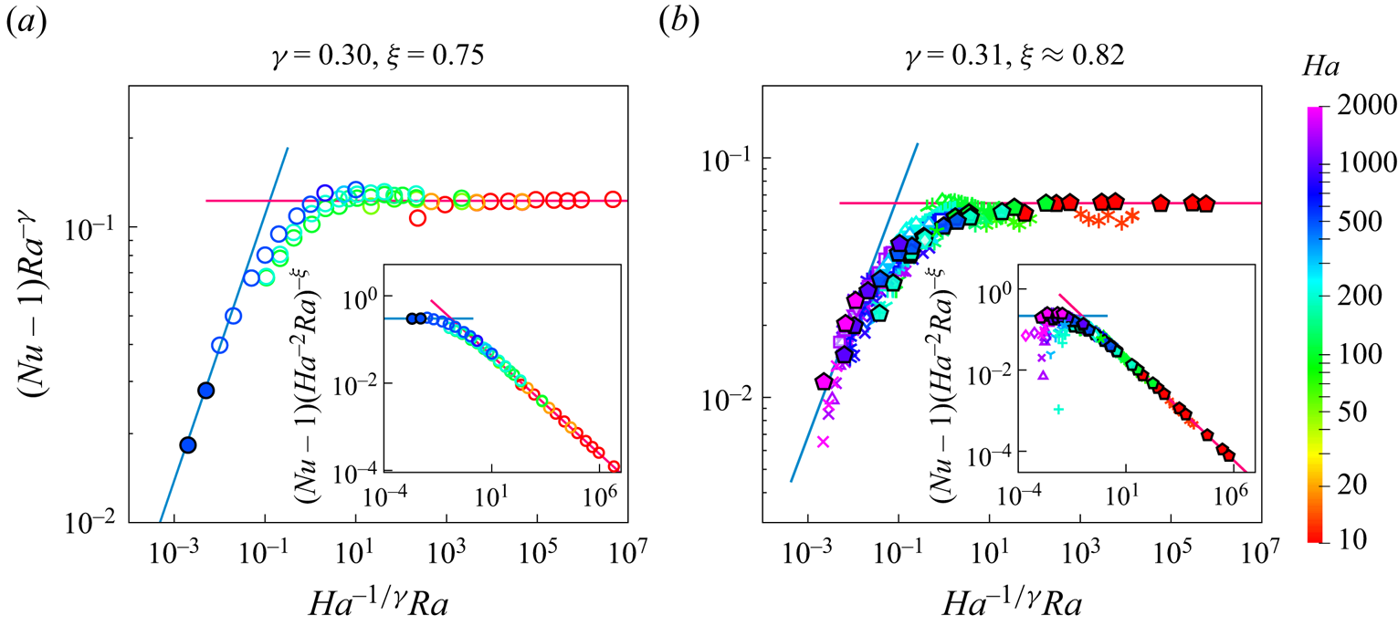
Figure 5. All data from figure 4 follow master scaling curves if plotted as figure 2 suggests, for (a)  $Pr=8$ and (b) $0.025\leq Pr \leq 0.029$. The values of $\gamma$ are calculated from GL theory, and the values of $\xi$ are calculated from (2.3). Pink and blue lines show the predictions of the slopes in the buoyancy and Lorentz-force-dominated regimes, respectively. The symbols have the same meaning as in figure 4.
4.1. Boundary layers
The model derivation relies on two key assumptions (§ 2): (i) laminar scaling of the BLs across the transition region and (ii) a cross-over of the respective scaling laws for the buoyancy- and the magnetically dominated regime for a  $Pr$-dependent ratio of BL thicknesses that does not implicitly depend on the control parameters, at least to a good approximation. In what follows we validate these assumptions against DNS data.
Concerning assumption (i), in a domain of height  $H$ over a semi-infinite plate, the average thermal BL thickness from laminar Prandtl–Blasius BL theory (Prandtl Reference Prandtl1905; Schlichting Reference Schlichting1979) is $\delta _T = 1/(2Nu)$, while the laminar viscous BL influenced by a vertical magnetic field is the Hartmann layer (Hartmann & Lazarus Reference Hartmann and Lazarus1937; Davidson Reference Davidson2016), $\delta _{\nu } = c /Ha$, where $c$ is a constant. For our data, values of $\delta _T$ and $\delta _T / \delta _\nu$ are provided in Appendix A, table 1. The BL thicknesses were determined by measurements of the slope of the mean temperature profile (Tilgner, Belmonte & Libchaber Reference Tilgner, Belmonte and Libchaber1993) and the mean horizontal velocity profile, respectively. The measured values of $\delta _T$ agree very well with the expected laminar scaling for all values of $Ha$ considered here, see table 1. In contrast, Hartmann-scaling $\delta _\nu \approx c H/Ha$ with $c \approx 1$ is attained only for $Ha \geq 200$ (not shown). In fact, deviations from Hartmann-scaling are expected at low $Ha$, as inertial forces dominate over the Lorentz force and the viscous BL is of Prandtl–Blasius type (Lim et al. Reference Lim, Chong, Ding and Xia2019). With increasing $Ha$ the Lorentz force eventually dominates the force balance and the Prandtl–Blasius BL transitions into the Hartmann layer. As can be seen from figure 5(b), the transitional regime requires $Ha \geq 200$ for the values of $Ra$ considered here. Similarly, according to the BL measurements for the $Pr = 8$ data (Lim et al. Reference Lim, Chong, Ding and Xia2019), $\delta _\nu = c/Ha$ with $c = 1.22$ for Hartmann numbers $Ha \geq 50$ which, according to the data presented in figure 5(a), covers the transitional and Lorentz-force dominated regimes and even extends into the buoyancy-dominated regime. As the transition between the two regimes is smooth and as $\delta _T=1/(2Nu)$ and $\delta _\nu =c/Ha$ are measured to a very good approximation for both the $Pr=8$ and the $Pr = 0.025$ data where relevant, we conclude that both relations hold across the transition region.
A formal way of stating assumption (ii) is to postulate the existence of two transition conditions at an intermediate point, where the influence of neither the Lorentz force or the buoyancy force can be ignored:
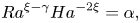 $$\begin{gather} Ra^{\xi-\gamma} Ha^{-2\xi} = \alpha, \end{gather}$$
 $$\begin{gather}\delta_T/\delta_\nu = \beta, \end{gather}$$
where  $\alpha = \alpha (Pr)$ and $\beta = \beta (Pr)$ only depend on $Pr$. To check if these relations hold, we use a bisection-type approach in combination with interpolation in $Ha$ and $Ra$ where required. We take an initial guess for $(\alpha, \beta )$, and for each value of $Ra$ (or $Ha$) we find the value of $Ha$ (or $Ra$) for which (4.2) holds, $Ha^*$ (or $Ra^*$), and see if this combination of $(Ra,Ha^*)$ (or $(Ra^*,Ha)$ ) satisfies (4.1). For the Lim et al. (Reference Lim, Chong, Ding and Xia2019) dataset at $Pr=8$, we find $\beta \approx 0.63$ and $\alpha \approx 11.24$ across a wide range of $Ra$, that is $(Ra,Ha^*) \in \{(10^7, 25.05), (10^8, 50), (10^9, 99.5), (10^{10}, 200.5)\}$. For the $Pr = 0.025$ data, we find $\beta \approx 33.33$ and $\alpha \approx 0.223$ satisfy these conditions for $(Ra^*,Ha) \in \{(1.32\times 10^6, 200), (2.49\times 10^7, 500), (2.34\times 10^8, 1000)\}$. We are unable to check this condition for lower $Ha$ since this requires a $Ra$ beneath the critical value for onset.
In summary, a BL cross-over is not observed during the transition. For the  $Pr = 8$ case, the transition occurs with the thermal BL nested within the Hartmann layer with $\delta _T/\delta _\nu \approx 0.63$, while the opposite applies for $Pr = 0.025$, where $\delta _T/\delta _\nu \approx 33.33$. In fact, we would expect the scaling cross-over to occur at a BL-thickness ratio $\delta _T/\delta _\nu \gg 1$ for small $Pr$, as temperature fluctuations play a more important role then. Furthermore, according to (3.1), both damping effects, that is momentum diffusion and the effect of the Lorentz force, are of less relevance at low $Pr$. That is, the transition to the buoyancy-dominated regime can be expected to occur at much lower thermal driving than at high $Pr$.
$Pr$.
5. Conclusion
In summary, we have proposed a heat transport model for the transition between the buoyancy- and Lorentz-force-dominated regimes of vertical MC. We validated the model using our DNS and data available in the literature. We wish to emphasise that the proposed model is parameter-free. For a given  $Pr$ and $Ra$ range, one can calculate the scaling exponent in the buoyancy-dominated regime, using GL theory. Then, using (2.3), one can calculate the scaling exponent $\xi$ in the Lorentz-force-dominated regime and collapse the data on a master curve by rescaling the coordinate axes as in figure 2. The model can in principle be extended to include the effect of a fluctuating magnetic field; this merely results in an adjustment of the prefactors.
Acknowledgements
The authors thank R.E. Ecke, D. Lohse and G.M. Vasil for fruitful discussions and R. Akhmedagaev for providing data.
Funding
The authors acknowledge the financial support from the Deutsche Forschungsgemeinschaft (SPP1881 ‘Turbulent Superstructures’ and grants Sh405/7, Sh405/16 and Li3694/1). This work used the ARCHER2 UK National Supercomputing Service (https://www.archer2.ac.uk) with resources provided by the UK Turbulence Consortium (EPSRC grants EP/R029326/1 and EP/X035484/1).
Declaration of interests
The authors report no conflict of interest.
Appendix A. Data table
Table 1. DNS details, where  $\sigma _{Nu}$ is the standard deviation of the Nusselt number $Nu$,
$Nu$,  $\delta _T$ and $\delta _\nu$ the thermal and viscous BL thicknesses, $N_x$, $N_y$, $N_z$ the number of nodes in x-, y- and z-direction, respectively; $T_{run}$ the number of free-fall times used for averaging; $\mathcal {N}_T$ and $\mathcal {N}_{Ha}$ the number of nodes within the thermal and Hartmann BLs; $h_{K}$ the Kolmogorov microscale, and $h_{DNS}/h_{K}$ the relative mean grid stepping. Grid refinement studies have been carried out for simulations marked by an asterisk.


 Open access